Nonholonomic deformation of KdV and mKdV equations and their symmetries, hierarchies and integrability

Abstract

Recent concept of integrable nonholonomic deformation found for the KdV equation is extended to the mKdV equation and generalized to the AKNS system. For the deformed mKdV equation we find a matrix Lax pair, a novel two-fold integrable hierarchy and exact N-soliton solutions exhibiting unusual accelerating motion. We show that both the deformed KdV and mKdV systems possess infinitely many generalized symmetries, conserved quantities and a recursion operator.

Short title: Integrable nonholonomic deformations of KdV and mKdV
PACS: 02.30.lk, 02.30.jr, 05.45.Yv, 11.10.Lm,
Key Words Integrable nonholonomic deformation, deformed mKdV, KdV and AKNS systems, Lax pair, accelerating N-soliton, two-fold integrable hierarchy, generalized symmetry, conservation law, recursion operator.

1 Introduction

Recently discovered integrable $6$-th order Korteweg de Vries (KdV) equation [1] was shown to represent a nonholonomic deformation (NHD) of the well known KdV equation preserving its integrability and exhibiting an integrable hierarchy [2]. In a subsequent development a matrix Lax pair, the N-soliton solution through inverse scattering transform (IST) method and an intriguing two-fold integrable hierarchy were found for this particular system by one of the authors [3]. The NHD of the KdV (dKdV) was shown recently to be a certain form of self-consistent source equation (SCSE) allowing particular exact solutions [4].

The NHD for such field theoretical models is given by a constraint in the form of nonlinear differential equation involving only $x$-derivatives on a single perturbing function, which is deforming the original integrable equation. This type of integrable deformation is a relatively recent discovery, which allows also an integrable hierarchy of higher order deformations. On the other hand the construction of SCSE is a well known concept [8], which is represented usually by a coupled system consisting of the original integrable equation with an additional term made from the eigenfunctions and 2N eigenvalue equations of the Lax operator with explicit dependence on N discrete eigenvalues. In general the eigenfunctions and eigenvalues are complex and one can also add another 2N number of evolution equations for the eigenfunctions. In a recent development of such SCSE its Rosochatius deformation is proposed [4]. At certain limit or at particular cases the contact between the lowest order NHD and the SCSE can be found, though the integrable hierarchy of higher order deformations seems to be possible only for the NHD.

In a slightly generalized form this deformed KdV equation can be given as

$$u_{t}-u_{xxx}-6uu_{x} = g_{x}(t,x),$$ (1)

$$g_{xxx}+4ug_{x}+2u_{x}(g+c(t)) = 0,$$ (2)

where subscript denote partial derivatives. Though the time-dependent arbitrary function $c(t)$ can be absorbed in equation (2) by redefining perturbing function $g(x,t)$, we keep it in the explicit form for our convenience. Recall that, the KdV and the modified KdV (mKdV) are intimately related partner systems [5]. Therefore it would be natural to expect that the concept of NHD found for the KdV should also be extendible to the mKdV equation. We show here that this expectation is indeed true by constructing explicitly a novel integrable NHD of the mKdV (dmKdV) equation, which can yield a new integrable 4th order potential mKdV equation. We discover for this integrable deformed mKdV equation with a nonholonomic constraint a matrix Lax pair, exact N-soliton solutions and a novel two-fold integrable hierarchy, similar to the result of the dKdV [3]. The solitons, found for both the basic field and the perturbing function of the dmKdV, show unusual accelerating (or decelerating) motion. We show that both the deformed KdV and mKdV systems possess infinitely many generalized symmetries and conserved quantities, and a recursion operator which have been studied until now only for their undeformed counterparts. The Lie symmetry analysis we perform here for the deformed equations leads also to explicit construction for the hierarchies of the generalized symmetries for both the basic field and the perturbing functions. Our analysis of the continuity equation for the dKdV and dmKdV reveals that the conserved densities for these deformed systems remain the same as in their original undeformed cases, whereas the current densities (fluxes) explicitly contain the deforming functions. This shows the intriguing fact that the nonholonomic deformations can appear only at the equation level, while the conserved integrals of motion remain the same under NHD.

Finally we unify dKdV and dmKdV to discover an integrable nonholonomic deformation for the more general AKNS [5] system.

The plan of the paper is as follows. In section $2$ the new NHD of the mKdV equation and the related integrability structures such as the matrix Lax pair and the exact $N$-soliton solution are presented. Tt is also shown that the dmKdV admits infinitely many higher order or generalized symmetries, conserved quantities and a recursion operator. In section $3$ a similar analysis has been carried out for the dKdV equation. Section $4$ generalizes the nonholonomic deformation to the AKNS system, revealing a novel two-fold integrable hierarchy for all its members and consequently for the dmKdV and the dKdV systems. In section $5$ we give a brief summary of our results and the concluding remarks.

2 Nonholonomic deformation of the mKdV equation

Integrable equations with NHD should be driven by an additional perturbative or deforming function, which in turn would be subjected to a differential constraint of nonholonomic nature. Therefore, analogous to the deformed KdV equation (1-2) we propose a deformed modified KdV equation with nonholonomic constraint as

$$v_{t}-v_{xxx}-6v^{2}v_{x}=w(t,x),$$ (3)

$$w_{x}-2v(c^{2}(t)-w^{2})^{\frac{1}{2}}=0.$$ (4)

Note that the arbitrary function $c(t)$ can be removed again from the equation (4) by rescaling $\frac{w(x,t)}{c(t)}\to w(x,t)$. We however keep $c(t)$ in the explicit form for the later convenience. At $c(t)=0$ we should have the deforming function $w(x,t)=0$, when the dmKdV (3-4) would reduce to the standard mKdV equation. For establishing the integrability of (3-4) we derive the associated pair of matrix Lax operators in the form

$$U(\lambda)=U^{mkdv}(\lambda),\ V(\lambda)=V^{mkdv}(\lambda)+V^{def}(\lambda),$$ (5)

where $U^{mkdv}(\lambda),V^{mkdv}(\lambda)$ are the well known Lax pair for the standard mKdV system [5]:

$$U^{mkdv}(\lambda) = i\lambda\sigma^{3}+iv\sigma^{1},$$

$$V^{mkdv}(\lambda) = 2i\lambda(v^{2}-2\lambda)\sigma^{3}-2i\lambda v_{x}\sigma^{2}+i(v_{xx}-4\lambda^{2}v+2v^{3})\sigma^{1},$$ (6)

while the additional term

$$V^{def}(\lambda)=\frac{i}{2\lambda}(b\sigma^{3}-w\sigma^{2}),\ \mbox{where }\ b=(c^{2}(t)-w^{2})^{\frac{1}{2}}$$ (7)

is responsible for the deformation of the mKdV equation. Here $\sigma^{a},\ a=1,2,3$ are standard Pauli matrices

$$\sigma^{1}=\left(\begin{array}[]{cc}0&1\\ 1&0\\ \end{array}\right),\ \sigma^{2}=\left(\begin{array}[]{cc}0&-i\\ i&0\\ \end{array}\right),\ \sigma^{3}=\left(\begin{array}[]{cc}1&0\\ 0&-1\\ \end{array}\right)$$ (8)

and $\sigma^{\pm}=\frac{1}{2}(\sigma^{1}\pm i\sigma^{2}).$ For confirming the Lax integrability of the NHD of the mKdV equation (3-4) we show that it is derivable from the flatness condition $U_{t}-V_{x}+[U,V]=0$ of the Lax pair (5). In this process one finds that, the expressions in all positive powers of $\lambda^{n},n=1,2,3$ vanishes trivially, while that for $n=0$ yields the deformed mKdV equation (3-4). The coefficients with the power $n=-1$ gives in turn the constraint equations

$$b_{x}=-2vw,\ \ w_{x}=2vb$$ (9)

from which eliminating function $b$ by using $b=(c^{2}(t)-w^{2})^{\frac{1}{2}}$ we arrive at the constraint (4) as required.

Note that one can also find a single higher order nonlinear equation by eliminating further the deforming function $w(x,t)$ from the set of equations (3-4). By introducing a potential field $\theta_{x}=2v$ we can rewrite Eq. (4) in the form $\theta_{x}=\frac{w_{x}}{(c^{2}-w^{2})^{\frac{1}{2}}},$ giving an easy solution $w=c(t)\sin\theta$, which can be checked by direct substitution, since $w_{x}=c\theta_{x}\cos\theta$ while ${(c^{2}-w^{2})^{\frac{1}{2}}}=c\cos\theta$. Inserting these expressions of $w$, $v$ and hence those of $v_{t},v_{xxx},v^{2}v_{x}$ through $\theta$ in Eq. (3) one can derive a new integrable 4-th order potential mKdV equation in $\theta$ given by

$$(\theta_{t}-\theta_{xxx}-\frac{1}{2}\theta_{x}^{3})_{x}=2c(t)\sin\theta.$$ (10)

Interestingly, keeping only the term $\theta_{xt}$ in the LHS, while grouping the other terms as

$$f(\theta)=(\theta_{xxx}+\frac{1}{4}\theta_{x}^{3})_{x},$$ (11)

one can rewrite Eq. (10) in the form of a perturbed sine-Gordon (SG) equation in the light-cone coordinates as

$$\theta_{xt}=2c(t)\sin\theta+f(\theta),$$ (12)

with a time-dependent mass parameter $m^{2}=2c(t)$, perturbed by a function (11). Significantly unlike most of the perturbed SG equation (12-11), derived here, is integrable allowing exact N-soliton solution. Thus the integrable higher order dmKdV equation (10) is equivalent to the NHD of the dmKdV equation (3-4), which in turn is equivalent to the set of equations (3) with (9).

2.1 Exact soliton solutions

As is well known any perturbation usually spoils the integrability of a nonlinear system and hence forbids general analytic solutions. However the dmKdV we have constructed retains its complete integrability in spite of the perturbation with nonholonomic constraint. Therefore exploiting this integrability property we intend to derive exact N-soliton solutions for the dmKdV equation (3-4) or equivalently for the novel 4-th order potential mKdV equation (10), through the IST method. The procedure follows that for the standard mKdV equation [6] in its initial steps, while in the final step the effect of deformation should be incorporated. It is intriguing to note from (5), that for the dmKdV equation, only the time Lax operator $V$ is deformed, while the space part $U$ is kept unchanged. This reveals an important connection between the deformed time evolution of the Jost solution and the NHD of the nonlinear equation.

Recall that for extracting the exact soliton solution in the IST the space-Lax operator $U(\lambda)$ describing the scattering of the Jost functions, plays the key role. Only at the final stage we need to fix the time evolution of the solitons through the time-dependence of the spectral data, which in turn is determined from the asymptotic value of the time-Lax operator $V(\lambda)|_{|x|\to\infty}$. Therefore following [6] we can derive the N-soliton solution for our deformed mKdV equation as

$$v(x)=[\frac{d^{2}}{dx^{2}}\ln detA(x)]^{\frac{1}{2}},$$ (13)

where the matrix function $A(x)$ is expressed through its elements as

$$A_{nm}=\sum_{l=1}^{N}f_{nl}f_{lm},\ \mbox{where}\ f_{nm}=\delta_{nm}+\frac{\beta_{n}\beta_{m}}{\kappa_{n}+\kappa_{m}}e^{-(\kappa_{n}+\kappa_{m})x}.$$ (14)

Here parameters $\kappa_{n},n=1,2,\ldots,N$, denote the time-independent zeros of the scattering matrix element: $a(\lambda=\lambda_{n})=0$, along the imaginary axis: $\lambda_{n}=i\kappa_{n}$ and $\beta_{n}(t)=b(\lambda=\lambda_{n})$ are the time-dependent spectral data to be determined from $V(\lambda)=V^{mkdv}(\lambda)+V^{def}(\lambda)$, at $x\to\pm\infty$.

Note that due to the boundary condition (BC) $v\to 0,w\to 0$ at $x\to\pm\infty$, the asymptotic value of (6): $V^{mkdv}(\lambda)\to-4i\lambda^{3}\sigma^{3}$ corresponds to the undeformed part, while the BC $b\to c(t)$ at $x\to\pm\infty$, determines the crucial effect of deformation $V^{def}(\lambda)\to\frac{i}{2}\lambda^{-1}c(t)\sigma^{3}$. As a result we obtain

$$\beta_{n}(t)=\beta_{n}(0)e^{(8\kappa_{n}^{3}t+\frac{\tilde{c}(t)}{\kappa_{n}})},\ \tilde{c}_{t}(t)=c(t),$$ (15)

yielding finally the $(x,t)$ dependent exact soliton solution from (14).

To see the effect of deformation on the dynamics of the solitons more closely we construct 1-soliton solution for the dmKDV equation as reduced from (13-15) at $N=1$:

$$v(x,t)=\frac{v_{0}}{2}{\rm sech}\xi,\ \xi=\kappa(x-vt)+\phi,\ v=v_{0}+v_{d}$$ (16)

where the phase $\phi$ is an arbitrary constant, $v_{0}=4\kappa^{2}$ is the usual constant velocity of the mKdV soliton, while $v_{d}=\frac{2\tilde{c}(t)}{v_{0}t}$ is the unusual time-dependent part of the velocity, induced by the deformation. Note that the time-dependent asymptotic value of the deformation acts here like a forcing term sitting at the space boundaries, which for $c(t)=c_{0}t$ with $c_{0}>0$ forces the soliton to accelerate, while with $c_{0}<0$ makes it decelerate (see Fig 1).

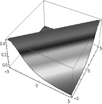
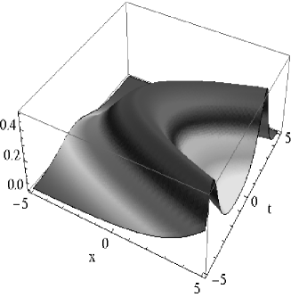
Figure 1: Exact soliton solutions in the (x,t)-plane: a) for the standard mKdV equation with constant soliton velocity (indicated by its constant inclination), b) for the nonholonomically deformed dmKdV equation with accelerated soliton (reflected in its curvature with $c(t)=0.5t$).

It is important to note, that the evolution of the basic field $v(x,t)$ comes here from two sources: $\partial_{t}v=\partial_{t_{0}}v+\partial_{t_{d}}v$, induced by two different ‘times’ $t_{0}$ and $t_{d}$. $\partial_{t_{0}}v=\partial_{t}v|_{c(t)=0}$ is the evolution due to the unperturbed time $t_{0}$, caused by the standard dispersive and nonlinear terms in (3), while $\partial_{t_{d}}v=c(t)\partial_{\tilde{c}(t)}v$ is the evolution due to the deformed time $t_{d}$, caused by the perturbation linked as

$$w=\partial_{t_{d}}v,\ \ b=c(t)+\int v\partial_{t_{d}}vdx.$$ (17)

Therefore using (17) and $\partial_{\tilde{c}(t)}\beta_{n}(t)=\frac{1}{\kappa}_{n}\beta_{n}(t)$ we can find from (13-15) the N-soliton solution corresponding to $w,b$, which for $N=1$ derived from (16) gives also localized accelerating solution

$$w(x,t)=c(t)\kappa{\rm sech}\xi{\rm tanh}\xi\ \mbox{and}\ b(x,t)=c(t)(1-\kappa^{2}{\rm sech}^{2}\xi).$$ (18)

This shows that the perturbing function, taking itself the solitonic form drives the field soliton to have an accelerated motion, while in turn the basic field solution self-consistently determines the solitonic form of the perturbing function, sustaining thus the integrability of the system.

2.2 Generalized symmetries

It is well known that the Lie symmetry analysis plays an effective role to study the integrability properties of nonlinear evolution equations in (1+1) dimensions such as the existence of infinitely many generalised symmetries, conserved quantities and a recursion operator ([9], [10], [11], [12], [13]). We show here that similar analysis can be performed with equal success for our deformed mKdV equation (3-4).

Note that the dmKdV equation is invariant under the scaling or dilatation symmetry

$$(t,x,v,w,c(t))\rightarrow(s^{-3}t,s^{-1}x,s^{1}v,s^{4}w,s^{4}c(t)),$$

where $s$ is an arbitrary parameter which suggests that $v$ corresponds to one derivative with respect to scaling $x$, $w$ corresponds to three derivatives with respect to $x$ and $c(t)$ corresponds to four derivatives with respect to $x$. We would like to mention that Hereman and his collaborators have developed an algorithm to derive generalised symmetries, conserved quantities and recursion operators for nonlinear partial differential and differential-difference equations [14]. Hereman’s algorithm is based basically on the concept of weights and ranks. The weight $W$ of a variable is defined as the exponent in the scaling parameter $s$ which multiplies the variable. Weights of the dependent variables are non-negative and rational. An expression is said to be uniform in rank if all its terms have the same rank. Setting $W(D)=W(\frac{\partial}{\partial x})=1$, we see that $W(v)=1,W(w)=4,W(b)=4,W(c(t))=4$ and $W(\frac{\partial}{\partial t})=3$ and hence eqn. (3) is of rank $4$ and (4) is of rank $5$. This property is called the uniformity in rank. The rank of a monomial is defined as the total weight of the monomial, again in terms of derivatives with respect to $x$.

Now, assume that the deformed mKdV equation (3-4) is invariant under one parameter nonpoint continuous transformations

$$t^{*}=t,\ \ x^{*}=x,\ \ v^{*}=v+\epsilon G_{i}+O(\epsilon^{2}),\ \ w^{*}=w+\epsilon H_{i}+O(\epsilon^{2}),$$ (19)

where

$$G_{i}=G_{i}(v,w,v_{x},v_{xx},v_{xxx},v_{4x},..,w_{x},w_{xx},\cdots)$$

$$H_{i}=H_{i}(v,w,v_{x},v_{xx},v_{xxx},v_{4x},..,w_{x},w_{xx},\cdots)$$

provided $v(x,t)$ and $w(x,t)$ satisfy equation (3- 4). Consequently we obtain the following invariant equations

$$\frac{DG_{i}}{Dt}=\frac{D^{3}G_{i}}{Dx^{3}}+6v^{2}\frac{DG_{i}}{Dx}+12vv_{x}G_{i}+\frac{DH_{i}}{Dx},$$ (20)

$$\frac{D^{2}H_{i}}{Dx^{2}}=2G_{i}\sqrt{(c(t)^{2}-w^{2})}-2vw\frac{\frac{DH_{i}}{Dx}}{\sqrt{(c(t)^{2}-w^{2})}},$$ (21)

where

$$\frac{D}{Dx}=\frac{\partial}{\partial{x}}+v_{x}\frac{\partial}{\partial{v}}+w_{x}\frac{\partial}{\partial{w}}+v_{xx}\frac{\partial}{\partial{v_{x}}}+v_{xt}\frac{\partial}{\partial{v_{t}}}+w_{xx}\frac{\partial}{\partial{w_{x}}}+w_{xt}\frac{\partial}{\partial{w_{t}}}+\cdots$$

$$\frac{D}{Dt}=\frac{\partial}{\partial{t}}+v_{t}\frac{\partial}{\partial{v}}+w_{t}\frac{\partial}{\partial{w}}+v_{xt}\frac{\partial}{\partial{v_{x}}}+v_{tt}\frac{\partial}{\partial{v_{t}}}+w_{xt}\frac{\partial}{\partial{w_{x}}}+w_{tt}\frac{\partial}{\partial{w_{t}}}+\cdots.$$

From equations (20-21), we see that

$$G_{1}=v_{x},\ \ \ H_{1}=w,$$ (22)

is a trivial generalized symmetry with rank $(2,4)$. This suggests that the next generalized symmetry $G_{2}$ and $H_{2}$ of dmKdV must have rank (4,6). With this in mind we first form monomials in $v$ and $w$ of rank $(4,6)$, Thus the most general form of $G_{2}$ and $H_{2}$ will be

$$G_{2}=a_{1}v^{2}v_{x}+a_{2}v_{3x}+a_{3}w,\ \ H_{2}=b_{1}v^{2}w+b_{2}w_{2x},$$ (23)

where $a_{i},b_{i},i=1,2,3$ are arbitrary constants to be determined. We now substitute $G_{2}$ and $H_{2}$ in the invariant equation (20-21),with $i=2$ and using (3-4) we find that the consistency condition holds only for the following parametric restrictions:

$$a_{1}=6,a_{2}=1,a_{3}=0,b_{1}=6,b_{2}=1$$

and so the generalized symmetry with rank $(4,6)$ becomes

$$G_{2}=6v^{2}v_{x}+v_{3x},\ \ \ H_{2}=6v^{2}w+w_{2x}.$$ (24)

Proceeding as above, for $i=3$, we find that the invariant equations (20-21) satisfy only if

$$G_{3}=v_{5x}+10v_{x}^{3}+40vv_{x}v_{2x}+10v^{2}v_{3x}+30v^{4}v_{x},\ \ \ \ \$$ (25)

$$H_{3}=w_{4x}+10v_{x}^{2}w+20vv_{2x}w+20vv_{x}w_{x}+10v^{2}w_{2x}+30v^{4}w,$$ (26)

which is a next nontrivial generalized symmetries with rank( 6,8). In a similar manner we can derive infinitely many generalized symmetries $\{(G_{4},H_{4}),(G_{5},H_{5}),\cdots\}$ for (3-4) with rank $\{(8,10),(10,12),\cdots\}$. We have also checked that the commutator

$$[G_{i},G_{i+1}]=0,[H_{i},H_{i+1}]=0,\ \ \forall\ i,$$

indicating that dmKdV eqn. (3-4) admits an infinitely many generalized symmetries which commute.

2.3 Recursion operator

In this section we derive a Recursion operator, an important property of the integrable systems, for our deformed mKdV eqn. (3-4), which is usually possible to obtain only for the unperturbed integrable systems. An operator valued function $\mathcal{R}$ is said to be a recursion operator of a scalar nonlinear partial differential equation with two independent variables if it satisfies

$$\tilde{G}=\mathcal{R}G,$$

where $\tilde{G}$ and $G$ are successive generalized symmetries. For (3-4) the above equation can be written as

$$\left[\begin{array}[]{c}G_{k+1}\\ H_{k+1}\\ \end{array}\right]=\mathcal{R}\left[\begin{array}[]{c}G_{k}\\ H_{k}\\ \end{array}\right]=\left(\begin{array}[]{cc}R_{;}{11}&R_{12}\\ R_{21}&R_{22}\\ \end{array}\right)\ \left[\begin{array}[]{c}G_{k}\\ H_{k}\\ \end{array}\right],$$ (27)

where $(G_{k},H_{k})$ and $(G_{k+1},H_{k+1})$ are successive generalized symmetries and $R_{ij},i,j=1,2$ are functions of dependent variable and their differential and integral operators. The construction of the recursion operator $\mathcal{R}$ for the dmKdV equation is as follows: For $k=2$ equation (27) becomes

$$\left[\begin{array}[]{c}G_{3}\\ H_{3}\\ \end{array}\right]=\left(\begin{array}[]{cc}R_{11}&R_{12}\\ R_{21}&R_{22}\\ \end{array}\right)\ \left[\begin{array}[]{c}G_{2}\\ H_{2}\\ \end{array}\right]$$ (28)

where $(G_{2},H_{2})$ and $(G_{3},H_{3})$ are the generalized symmetries of ranks $(4,6)$and $(6,8)$ respectively. The ranks of $R_{11},R_{12},R_{21}$ and $R_{22}$ can be determined from the following relations

$$rankG_{3}=rankR_{11}+rankG_{2}=rankR_{12}+rankH_{2},$$ (29)

$$rankH_{3}=rankR_{21}+rankG_{2}=rankR_{22}+rankH_{2},$$ (30)

Equations (29-30) show that the ranks of $R_{11},R_{12},R_{21},R_{22}$ respectively are $2,0,4,2$ and so we consider the entries of $\mathcal{R}$ written in terms of differential and integral operators of the dependent variables having the form

$$R_{11} = c_{0}\partial^{2}+c_{1}v^{2}+c_{2}v_{x}\partial^{-1}v,\ R_{12}=0,\ R_{22}=g_{0}\partial^{2}+g_{1}v^{2}+g_{2}v\partial^{-1}v_{x},$$

$$R_{21} = f_{0}w\partial^{-1}v+f_{1}v\partial^{-1}w+f_{2}v^{4}+f_{3}w+f_{4}v_{4x}\partial^{-1}+f_{5}v^{2}\partial^{2},$$ (31)

where$c_{i},g_{i},i=0,1,2$ and $f_{j},j=0,1,2,3,4,5$ are constants to be determined. Substituting the above in (28) we find that it is satisfied identically only if

$$c_{0}=1,c_{1}=4,c_{2}=4,f_{0}=4,f_{1}=4,f_{2}=f_{3}=f_{4}=f_{5}=0,g_{0}=1,g_{1}=4,g_{2}=-4$$

and therefore the recursion operator for the dmKdV equation becomes

$$\mathcal{R}=\left(\begin{array}[]{cc}\partial^{2}+4v^{2}+4v_{x}\partial^{-1}v&0\\ 4w\partial^{-1}v+4v\partial^{-1}w&\partial^{2}+4v^{2}-4v\partial^{-1}v_{x}\\ \end{array}\right).$$ (32)

2.4 Conserved quantities

A local conservation law of a partial differential equation with two independent variables $(x,t)$ is defined by

$$\frac{\partial}{\partial t}\rho+\frac{\partial}{\partial x}J=0$$ (33)

which is satisfied on all solutions. The function $\rho(x,t)$ is usually called local conserved density and $J(x,t)$ is the associated flux also known as current density. We show that the dmKdV (3-4) or eqn.(3) and (8) admit infinitely many polynomial conserved quantities. From (3), we find directly that

$$\rho[1]=v,\ \ \ \ J[1]=-(v_{xx}+2v^{3}+\int dxw)$$ (34)

is a trivial conserved quantity with rank $(1,3)$. Recall that (3) and (8) is invariant under scaling symmetry  $(t,x,v,w,b,c)\rightarrow(s^{-3}t,s^{-1}x,s^{1}v,s^{4}w,s^{4}b,s^{4}c),\$ where $s$ is an arbitrary parameter. To derive a conserved quantity with rank $(2,4)$, as before, we form monomials of $v(x,t)$ and $w(x,t)$ which gives the list $\mathcal{L}_{1}=\{v^{2}\}$. Thus the conserved density of rank 2 will be $\rho(x,t)=v^{2}.$ As a result we obtain

$$\rho[2]=v^{2},\ \ J[2]=-2vv_{xx}-3v^{4}+v_{x}^{2}+b.$$ (35)

Proceeding as above we find the next two conserved quantities as

$$\rho[3]=v^{4}-v_{x}^{2},J[3]=-4v^{6}-4v^{3}v_{xx}+2v_{x}v_{xxx}-v_{xx}^{2}+12v^{2}v_{x}^{2}+2v^{2}b,$$ (36)

$$\rho[4] = v^{6}-5v^{2}v_{x}^{2}+\frac{1}{2}v_{xx}^{2},$$ (37)

$$J[4] = \frac{-9}{2}v^{8}-6v^{5}v_{xx}+10v^{2}v_{x}v_{xxx}-v_{xx}v_{4x}+\frac{1}{2}v_{xxx}^{2}-8v^{2}v_{xx}^{2}$$ (38)

$$+ 45v^{4}v_{x}^{2}-10vv_{x}^{2}v_{xx}-\frac{1}{2}v_{x}^{4}+3v^{4}b-v_{x}^{2}b-2vv_{x}b_{x}.$$

with ranks (4,6) and (6,8) respectively. In a similar manner we can derive an infinitely many conserved quantities $(\rho(x,t),J(x,t))$ for dmKdV with ranks $\{(8,10),(10,12)\ldots\}$ which involve lengthy expressions and so the details are omitted here.

It is important to notice that the integrals of motion describing infinite number of integrated conserved quantities $c_{n},\ n=1,2,\ldots$, which should be commutative as a necessary criterion of Liouville integrability can be given by $c_{n}=\int\rho[n]dx$. It is clearly seen from the continuity equation (33) that due to vanishing of the fields along with their derivatives at the space-infinities we naturally obtain $\partial_{t}c_{n}=0$. Therefore from the expressions of $\rho[n],n=1,2,\ldots$, derived above we get the conserved quantities for the dmKdV equation as

$$c_{1}=\int vdx,\ c_{2}=\int v^{2}dx,\ c_{3}=\int(v^{4}-v_{x}^{2})dx$$ (39)

with $c_{3}=H_{mkdv}$ being the Hamiltonian of the mKdV equation. We see therefore that the conserved quantities including the Hamiltonian remains the same for both the deformed and undeformed mKdV systems, though the corresponding equations for the dmKdV with additional perturbing function and nonholonomic constraint on it are surely different. Note also that this effect of deformation changes the structure of the local current densities $J[n],n=1,2,\ldots$, which contain the deforming functions $w,b$, but not the densities $\rho[n]$, which generate the conserved quantities.

3 Nonholonomic deformation of the KdV equation and its integrability aspects

Nonholonomic constraints on field models have received increasing attention over recent years , while a significant breakthrough is made recently by discovering an integrable nonholonomic deformation for the KdV equation [1, 2, 3, 4]. It has been established that this deformed KdV equation like the undeformed standard KdV admits Lax pair, N-soliton solutions and a two-fold integrable hierarchy [3]. The deformed KdV can be considered also as a source equation [4], which is however different from and simpler than the well known source KdV equation [8]. The novelty of this source is that it can be deformed recursively by going to the next order in its integrable hierarchy with higher order deformations [3, 7].

However many other fundamental and important properties of the integrable systems, such as the existence of an infinite number of generalized symmetries, conserved quantities and a recursion operator, which have been well established for the standard KdV equation have not yet been studied for their nonholonomically deformed extension, investigation of which is therefore our aim here.

3.1 Generalized symmetries

The deformed KdV equation (1-2) is obviously invariant under the dilatation symmetry

$$(t,x,u,g,c(t))\rightarrow(s^{-3}t,s^{-1}x,s^{2}u,s^{4}g,s^{4}c(t)),$$ (40)

where $s$ is an arbitrary parameter which suggests that $u$ corresponds to two derivatives, while both $g$ and $c(t)$ correspond to four derivatives, with respect to $x$. Setting $W(D)=W(\frac{\partial}{\partial x})=1$, therefore one gets $W(u)=2,W(g)=4,W(c(t))=4$ and $W(\frac{\partial}{\partial t})=3$ and hence equations (1-2) is of rank $(5,7)$. This property is called the uniformity in rank. Now, assume that the deformed KdV equation (1-2) is invariant under one parameter continuous nonpoint transformations

$$u^{*}=u+\epsilon G_{i}+O(\epsilon^{2}),$$ (41)

$$g^{*}=g+\epsilon H_{i}+O(\epsilon^{2}),$$ (42)

where

$$G_{i}=G_{i}(u,g,u_{x},u_{xx},u_{xxx},u_{4x},..,g_{x},g_{xx},\cdots)$$

$$H_{i}=H_{i}(u,g,u_{x},u_{xx},u_{xxx},u_{4x},..,g_{x},g_{xx},\cdots)$$

provided $u(x,t)$ and $g(x,t)$ satisfy equations (1-2). Consequently we obtain the following invariant equations

$$\frac{DG_{i}}{Dt}=\frac{D^{3}G_{i}}{Dx^{3}}+6u\frac{DG_{i}}{Dx}+6u_{x}G_{i}+\frac{DH_{i}}{Dx},$$ (43)

$$\frac{D^{3}H_{i}}{Dx^{3}}+4u\frac{DH_{i}}{Dx}+4G_{i}g_{x}+2\frac{DG_{i}}{Dx}(g+c(t))+2u_{x}H_{i}=0.$$ (44)

From (43-44) we derive the following generalized symmetries

$$G_{1}=u_{x},H_{1}=g_{x}\ \ G_{2}=6uu_{x}+u_{3x},H_{2}=6ug_{x}+g_{3x},$$ (45)

which are trivial ones with ranks $(3,5)$ and $(5,7)$, respectively. Proceeding as before we find that (1- 2) admits an infinitely many generalized symmetries, where the first two nontrivial generalised symmetries are

$$G_{3}=30u^{2}u_{x}+20u_{x}u_{xx}+10uu_{3x}+u_{5x},$$

$$H_{3}=30u^{2}g_{x}+10u_{x}g_{xx}+10u_{2x}g_{x}+10ug_{3x}+g_{5x},$$

and

$$G_{4}=140u^{3}u_{x}+70u_{x}^{3}+280uu_{x}u_{2x}+70u^{2}u_{3x}+70u_{2x}u_{3x}+42u_{x}u_{4x}+14uu_{5x}+u_{7x}$$

$$H_{4}=140u^{3}g_{x}+70u_{x}^{2}g_{x}+140uu_{x}g_{2x}+140uu_{2x}g_{x}+70u^{2}g_{3x}$$

$$\hskip 42.67912pt+42u_{2x}g_{3x}+28u_{3x}g_{2x}+28u_{x}g_{4x}+14u_{4x}g_{x}+14ug_{5x}+g_{7x}$$

with ranks $(7,9)$ and $(9,11)$, respectively. Note that the remaining higher order generalised symmetries involve lengthy expressions and hence not presented here. We find also that the commutator relations

$$[G_{i},G_{i+1}]=0,\ \ \ [H_{i},H_{i+1}]=0,\forall i$$

hold. It is straightforward again to check that the derived generalised symmetries satisfy

$$\left[\begin{array}[]{c}G_{i+1}\\ H_{i+1}\\ \end{array}\right]=\mathcal{R}\left[\begin{array}[]{c}G_{i}\\ H_{i}\\ \end{array}\right]\forall i,$$

with the recursion operator

$$\mathcal{R}=\left(\begin{array}[]{cc}\partial^{2}+4u+2u_{x}\partial^{-1}&0\\ 2g_{x}\partial^{-1}+2\partial^{-1}g_{x}&\partial^{2}+4u-2\partial^{-1}u_{x}\\ \end{array}\right).$$ (46)

3.2 Conserved quantities

Recall that the dKdV equation (1-2) is invariant under the dilatation symmetry $(t,x,u,g)\rightarrow(s^{-3}t,s^{-1}x,s^{2}u,s^{4}g).$ We can show again that the dKdV equation admits an infinitely many conserved quantities. From (1-2), we find that

$$\rho[1]=u,\ \ J[1]=-(u_{xx}+3u^{2}+g)$$ (47)

correspond to a trivial conserved quantity with rank $(2,4)$. To derive the next conserved quantity with rank $(4,6)$ we form monomials of $u$ and $g$ as before, which give the list $\mathcal{L}_{1}=\{u^{2},u_{xx}\}$. Thus the most general form of the conserved density of rank 4 would be  $\rho(x,t)=c_{1}u^{2}+c_{2}u_{xx},$  with $c_{1}$, $c_{2}$ are constants. It is straightforward to check that the next order conserved density and associated flux

$$\rho[2]=u^{2},\ J[2]=(-4u^{3}-2uu_{xx}+u_{x}^{2}+2ug+g_{xx}+2uc(t))$$ (48)

satisfy (33). In a similar manner we obtain in the next higher order

$$\rho[3]=(4u^{3}-2u_{x}^{2}),\ J[3]=(-18u^{4}+24uu_{x}^{2}-12u^{2}u_{xx}-2u_{xx}^{2}+4u_{x}u_{3x}$$

$$-g_{4x}+4u^{2}g+4u^{2}c(t)-2u_{xx}c(t)-2u_{xx}g-6u_{x}g_{x}).$$ (49)

We wish to add that the next higher order conserved quantities involve lengthy expressions and so we refrain from presenting them.

We can obviously construct the commuting family of integrated conserved quantities as above: $c_{n}=\int\rho[n]dx$ with $\partial_{t}c_{n}=0$. Therefore from the corresponding $\rho[n],n=1,2,\ldots$, we get the conserved quantities for the dKdV equation as

$$c_{1}=\int u\ dx,\ c_{2}=\int u^{2}\ dx,\ c_{3}=\int(4u^{3}-2u_{x}^{2})dx,...$$ (50)

with $c_{3}=H_{kdv}$ being the Hamiltonian of the KdV equation. Therefore we see again that for the deformed KdV system, the conserved quantities remain the same as in the undeformed case, though the corresponding equation gets deformed due to the nonholonomic constraint.

4 Generalization to the nonholonomic deformation of the AKNS system

In sect. 2 we have discovered a new integrable nonholonomic deformation of the mKdV system, extending the dKdV. Here we intend to show that these deformed systems can be unified and generalized further to an integrable nonholonomic deformation of the AKNS [5] system:

$$q_{t}-q_{xxx}-6(qr)q_{x}=g_{x},$$ (51)

$$r_{t}-r_{xxx}-6(qr)r_{x}=f_{x}.$$ (52)

For finding the integrable nonholonomic constraints on the deforming functions $g,f$ we introduce the deforming matrix $G^{(1)}=g\sigma^{+}+f\sigma^{-}+b\sigma^{3}$ and similarly for $G^{(2)}$, and denote the AKNS fields in the matrix form $U^{(0)}=q\sigma^{+}+r\sigma^{-}$. Integrability condition, i.e. the flatness condition of the associated deformed Lax pair (with the additional deformation $V^{(def)}_{2}(\lambda)=\frac{i}{2}(\lambda^{-1}G^{(1)}+\lambda^{-2}G^{(2))}$), therefore leads to the nonholonomic constraint:

$$G^{(1)}_{x}=i[U^{(0)},G^{(1)}]+i[\sigma_{3},G^{(2)}],\ G^{(2)}_{x}=i[U^{(0)},G^{(2)}].$$ (53)

Higher order integrable deformations can be generated recursively by adding to $V^{(def)}_{2}(\lambda)$ more terms like $\frac{i}{2}\lambda^{-j}G^{(j)},j=3,\ldots n$ with arbitrary $n$. It would result to a new integrable hierarchy of nonholonomic deformations of the AKNS (dAKNS) system, given explicitly through the higher order constraints

$$G^{(1)}_{x} = i[U^{(0)},G^{(1)}]+i[\sigma_{3},G^{(2)}],\ \ldots\ ,$$

$$G^{(n-1)}_{x} = i[U^{(0)},G^{(n-1)}]+i[\sigma_{3},G^{(n)}],$$

$$G^{(n)}_{x} = i[U^{(0)},G^{(n)}].$$ (54)

For $n=1$ this hierarchy clearly reduces to

$$G^{(1)}_{x}=i[U^{(0)},G^{(1)}],$$ (55)

while for $n=2$ gives (53).

The integrability of the dAKNS system (51-53) is guaranteed from its associated matrix Lax pair

$$U(\lambda) = i\lambda\sigma^{3}+iU^{(0)},\ U^{(0)}=q\sigma^{+}+r\sigma^{-},$$

$$V(\lambda) = V^{AKNS}(\lambda)+V^{def}(\lambda),$$ (56)

where

$$V^{AKNS}(\lambda) = iU^{(0)}_{xx}-4i\lambda^{3}\sigma^{3}+2\sigma^{3}\lambda(-U^{(0)}_{x}+i(U^{(0)})^{2})-4iU^{(0)}\lambda^{2}$$

$$+ 2i(U^{(0)})^{3}-[U^{(0)},U^{(0)}_{x}],$$

$$V^{def}(\lambda) = \frac{1}{2}(\lambda^{-1}G^{(1)}+\lambda^{-2}G^{(2)}).$$ (57)

We can check that the flatness condition $U_{t}-V_{x}+[U,V]=0$ of this Lax pair yields the dAKNS system (51-53). Note that we can generate a novel two-fold integrable hierarchy for this deformed AKNS system. Firstly, by keeping the perturbed equations (51-52) the same, but by increasing the order of the differential constraint recursively as (54), we obtain a new integrable hierarchy for the dAKNS. Secondlly, by keeping the constraint fixed to its lowest level, i.e. as (55) or (53), one can increase also the order of the AKNS equation with higher dispersions in the lefthand side of (51-52) in the standard way, generating another integrable hierarchy.

This general deformed AKNS system along with its two-fold integrable hierarchy proposed here can yield as particular cases both the dmKdV and the dKdV equations considered above. One can check that the dmKdV equation proposed here can be obtained directly from the dAKNS through the reduction $q=r=v$, which degenerates (51-52) to the same equation (3), while the constraint (4) is derived from (55) with

$$G^{(1)}=i(c^{2}(t)-w^{2})^{\frac{1}{2}}\sigma^{3}+iw\sigma^{2},\ \ G^{(2)}=0.$$ (58)

Similarly for deriving the dKdV from the general case of dAKNS system we have to consider the particular reduction $q=u,r=1$ , which obviously makes (52) trivial while reduces (51) to the deformed KdV (1). At the same time the constraint (2) can be derived by solving (53) as

$$G^{(1)} = i(g+c)\sigma^{3}-g_{x}\sigma^{+}$$

$$G^{(2)} = \frac{g_{x}}{2}\sigma^{3}+i(g+c)\sigma^{-}+e\sigma^{+},\ e_{x}=iug_{x},$$ (59)

where $u(x,t)$ is the KdV field and $(x,t)$ is the deforming function with $c(t)$ as its asymptotic value $\lim_{|x|\to\infty}g(x,t)=c(t)$.

Reductions of the deformed AKNS system to other important integrable deformations, e.g. NHD of the nonlinear Schrödinger and sine-Gordon equations have been considered in [7].

5 Concluding remarks

We have extended the concept of nonholonomic deformation from the KdV equation to the mKdV equation and constructed for this novel deformed system all essential and important structures of an integrable system, like a matrix Lax pair, exact N-soliton solution through IST, integrable hierarchies etc. Interestingly. the integrable deformed mKdV, that we have discovered here, shows even a richer picture than that of the usual integrability.

In particular, it allows accelerating exact solitons for the basic field as well as for the perturbing function. The perturbing function, similar to the deformed KdV case [3], takes a consistent solitonic form and forces the field soliton through its asymptotic value $c(t)$ at space infinities, to move with an acceleration (or deceleration). Therefore such a self consistent solitonic perturbation, which preserves the integrability, could be significantly important in laboratory experiments with mKdV solitons, where the usual loss of energy inevitable in a realistic system could be compensated for by the driving force given from the boundaries as found here.

Moreover, the deformed mKdV system shows a novel two-fold integrable hierarchy, as found also for the deformed KdV [3]. The first one corresponds to the standard mKdV hierarchy with higher dispersions but perturbed with a deforming function subjected to a given nonholonomic constraint. The second one is a new hierarchy of equations, where the same mKdV equation is perturbed now by a function with increasingly higher order of nonholonomic constraint.

In parallel with the established procedure for finding the symmetries of the integrable equations, we have constructed for the first time an infinite number of generalized symmetries, conserved quantities and a recursion operator for both the deformed KdV and the deformed mKdV equations. It reveals a remarkable fact that, though the deforming functions are contained in local current densities, the local densities do not have any dependence on them. Hence the integrated conserved quantities are also not influenced by the deformation and remain the same as in the unperturbed case.

Finally we have unified and generalized the deformed KdV and mKdV equations to the deformed AKNS system, with explicit construction of its Lax pair and a two-fold integrable hierarchy. Particular reductions of this new deformed integrable AKNS system yield the deformed KdV as well as the deformed mKdV system presented here.

The study of the deformed Painlevé class of equations obtained as reductions of the dKdV and dmKdV equations, a potentially important project, we wish to pursue further.

References

- [1] A.Karasu-Kalkanli, A.Karasu, A.Sakovich, S.Sakovich, and R.Turhan , A new integrable generalization of the Korteweg-de-Vries equation J.Math.Phys. 49,073516 (2008).
- [2] B.A.Kupershmidt,KdV6: An integrable system Phys. Lett. A372, 2634 (2008).
- [3] A.Kundu, Exact accelerating solitons in nonholonomic deformation of the KdV equation with two-fold integrable hierarchy, J. Phys. A: Math. Theor. 41, 495201 (2008).
- [4] Yuqin Yao, Yunbo Zeng, The bi-Hamiltonian structure and new solutions of KdV6 equation, arXiv:0810.1986[nlin.SI] Oct 14, 2008.
- [5] M. J. Ablowitz, D.J.Kaup, A.C.Newell and H. Segur, The inverse scattering transform - Fourier analysis for nonlinear problems, Stud.Appl.Math. 53 249 (1974).
- [6] M. Wadati, The exact solution of the modified Korteweg-de Vries equation J. Phys. Soc. Jpn., 32, 1681 (1972)
- [7] A.Kundu,Nonlinearizing linear equations to integrable systems including new hierarchies with nonholonomic deformations terms,arxiv:0711.0878v3, 16 Jun 2008.
- [8] V. K. Melnikov,Integration method of the KdV equation with a self-consistentl source , Phys. Lett. A133, 493 (1988).
- [9] L.V.Ovisannikov, Group Analysis of Differential Equations, Academic Press, NewYork (1982).
- [10] P.J.Olver,Applications of Lie Groups to Differential Equations, Springer, Berlin, (1986).
- [11] G.Bluman and S.Kumei, Symmetries and Differential Equations, Springer,Berlin (1989).
- [12] A.S.Fokas,Symmetries and integrability, Stud. Appl. Math. 77, 253 (1987).
- [13] M.Lakshmanan and P. Kaliappan, Lie transformations, nonlinear evolution equations and Painlevé forms J.Math.Phys.24 , 795 (1983).
- [14] W. Hereman, J.A. Sanders, J.Sayers and J.P.Wang,Symbolic computation of polynomial conserved densities, generalised symmetries and recursion operators for nonlinear differential- difference equations,In: Group Theory and Numerical Analysis, CRM Proccedings and Lecture Series 39 Eds. P.Winternitz etal, Americal Mathematical Society, 267 (2005).