Self-sustained traversable wormholes in noncommutative geometry

Abstract

In this work, we find exact wormhole solutions in the context of noncommutative geometry, and further explore their physical properties and characteristics. The energy density of these wormhole geometries is a smeared and particle-like gravitational source, where the mass is diffused throughout a region of linear dimension $\sqrt{\alpha}$ due to the intrinsic uncertainty encoded in the coordinate commutator. Furthermore, we also analyze these wormhole geometries considering that the equation governing quantum fluctuations behaves as a backreaction equation. In particular, the energy density of the graviton one loop contribution to a classical energy in a traversable wormhole background and the finite one loop energy density is considered as a self-consistent source for these wormhole geometries. Interesting solutions are found for an appropriate range of the parameters, validating the perturbative computation introduced in this semi-classical approach.

I Introduction

An interesting development of string/M-theory has been the necessity for spacetime quantization, where the spacetime coordinates become noncommuting operators on a $D$-brane Witten . The noncommutativity of spacetime is encoded in the commutator $\left[\mathbf{x}^{\mu},\mathbf{x}^{\nu}\right]=i\,\theta^{\mu\nu}$, where $\theta^{\mu\nu}$ is an antisymmetric matrix which determines the fundamental discretization of spacetime. It has also been shown that noncommutativity eliminates point-like structures in favor of smeared objects in flat spacetime Smailagic:2003yb . Thus, one may consider the possibility that noncommutativity could cure the divergences that appear in general relativity. The effect of the smearing is mathematically implemented with a substitution of the Dirac-delta function by a Gaussian distribution of minimal length $\sqrt{\alpha}$. In particular, the energy density of a static and spherically symmetric, smeared and particle-like gravitational source has been considered in the following form Nicolini:2005vd

$$\rho_{\alpha}(r)=\frac{M}{(4\pi\alpha)^{3/2}}\;\mathrm{exp}\left(-\frac{r^{2}}{4\alpha}\right)\,,$$ (1)

where the mass $M$ is diffused throughout a region of linear dimension $\sqrt{\alpha}$ due to the intrinsic uncertainty encoded in the coordinate commutator.

In this context, the Schwarzschild metric is modified when a non-commutative spacetime is taken into account Nicolini:2005vd ; Esposito . The solution obtained is described by the following spacetime metric

$$ds^{2}=-f(r)\,dt^{2}+\frac{dr^{2}}{f(r)}+r^{2}\,(d\theta^{2}+\sin^{2}{\theta}\,d\phi^{2})\,,$$ (2)

where the factor $f(r)$ is defined as

$$f(r)=\left[1-\frac{2r_{S}}{r\sqrt{\pi}}\gamma\left(\frac{3}{2},\frac{r^{2}}{4\alpha}\right)\right]\,,$$ (3)

and

$$\gamma\left(\frac{3}{2},\frac{r^{2}}{4\alpha}\right)=\int\limits_{0}^{r^{2}/4\alpha}dt\sqrt{t}\exp\left(-t\right)$$ (4)

is the lower incomplete gamma function, $r_{S}=2MG$ is the Schwarzschild radius Nicolini:2005vd . The classical Schwarzschild mass is recovered in the limit $r/\sqrt{\alpha}\rightarrow\infty$. It was shown that the coordinate noncommutativity cures the usual problems encountered in the description of the terminal phase of black hole evaporation. More specifically, it was found that the evaporation end-point is a zero temperature extremal black hole and there exist a finite maximum temperature that a black hole can reach before cooling down to absolute zero. The existence of a regular de Sitter at the origin’s neighborhood was also shown, implying the absence of a curvature singularity at the origin. Recently, further research on noncommutative black holes has been undertaken, with new solutions found providing smeared source terms for charged and higher dimensional cases newNCGbh .

In this paper we extend the above analysis to wormhole geometries. In classical general relativity, wormholes are supported by exotic matter, which involves a stress energy tensor that violates the null energy condition (NEC) Morris:1988cz . Several candidates have been proposed in the literature, amongst which we refer to the first solutions with what we now call massless phantom scalar fields Ellis-Bronn ; solutions in higher dimensions, for instance in Einstein-Gauss-Bonnet theory EGB ; wormholes on the brane braneWH ; solutions in Brans-Dicke theory Nandi:1997en ; wormhole solutions in semi-classical gravity (see Ref. Garattini:2007ff and references therein); exact wormhole solutions using a more systematic geometric approach were found Boehmer:2007rm ; solutions supported by equations of state responsible for the cosmic acceleration phantomWH ; and NEC respecting geometries were further explored in conformal Weyl gravity Lobo:2008zu , etc (see Refs. Lemos:2003jb ; Lobo:2007zb for more details and Lobo:2007zb for a recent review).

In this context, we shall also be interested in the analysis that these wormholes be sustained by their own quantum fluctuations. As wormholes violate the NEC, and consequently violate all of the other classical energy conditions, it seems that these exotic spacetimes arise naturally in the quantum regime, as a large number of quantum systems have been shown to violate the energy conditions, such as the Casimir effect. Indeed, various wormhole solutions in semi-classical gravity have been considered in the literature semiclassWH . In this work, we consider the formalism outlined in detail in Ref. Garattini ; Garattini:2007ff , where the graviton one loop contribution to a classical energy in a wormhole background is used. The latter contribution is evaluated through a variational approach with Gaussian trial wave functionals, and the divergences are treated with a zeta function regularization. Using a renormalization procedure, the finite one loop energy was considered a self-consistent source for a traversable wormhole.

This paper is outlined in the following manner: In Section II, we consider traversable wormholes in noncommutative geometry, by analyzing the field equations and the characteristics and properties of the shape function in detail. In Section III, we analyze these wormhole geometries in semi-classical gravity, considering that the equation governing quantum fluctuations behaves as a backreaction equation. Finally, in Section IV, we conclude.

II Traversable wormholes in noncommutative geometry

II.1 Metric and field equations

Consider the following static and spherically symmetric spacetime metric

$$ds^{2}=-e^{2\Phi(r)}\,dt^{2}+\frac{dr^{2}}{1-b(r)/r}+r^{2}\,(d\theta^{2}+\sin^{2}{\theta}\,d\phi^{2})\,,$$ (5)

which describes a wormhole geometry with two identical, asymptotically flat regions joined together at the throat $r_{0}>0$. $\Phi(r)$ and $b(r)$ are arbitrary functions of the radial coordinate $r$, denoted as the redshift function and the shape function, respectively. The radial coordinate has a range that increases from a minimum value at $r_{0}$, corresponding to the wormhole throat, to $\infty$.

Using the Einstein field equation, $G_{\mu\nu}=8\pi G\,T_{\mu\nu}$ (with $c=1$), we obtain the following stress-energy tensor scenario

$$\rho(r) =\frac{1}{8\pi G}\;\frac{b^{\prime}}{r^{2}}\,,$$ (6)

$$p_{r}(r) =\frac{1}{8\pi G}\left[2\left(1-\frac{b}{r}\right)\frac{\Phi^{\prime}}{r}-\frac{b}{r^{3}}\right]\,,$$ (7)

$$p_{t}(r) =\frac{1}{8\pi G}\left(1-\frac{b}{r}\right)\Bigg{[}\Phi^{\prime\prime}+(\Phi^{\prime})^{2}$$

$$-\frac{b^{\prime}r-b}{2r(r-b)}\Phi^{\prime}-\frac{b^{\prime}r-b}{2r^{2}(r-b)}+\frac{\Phi^{\prime}}{r}\Bigg{]}\,,$$ (8)

in which $\rho(r)$ is the energy density, $p_{r}(r)$ is the radial pressure, and $p_{t}(r)$ is the lateral pressure measured in the orthogonal direction to the radial direction. Using the conservation of the stress-energy tensor, $T^{\mu\nu}{}_{;\nu}=0$, we obtain the following equation

$$p_{r}^{\prime}=\frac{2}{r}\,(p_{t}-p_{r})-(\rho+p_{r})\,\Phi^{\prime}\,.$$ (9)

Note that Eq. $\left(\ref{prderivative}\right)$ can also be obtained from the field equations by eliminating the term $\Phi^{\prime\prime}$ and taking into account the radial derivative of eq. $\left(\ref{prWH}\right)$.

Another fundamental property of wormholes is the violation of the null energy condition (NEC), $T_{\mu\nu}k^{\mu}k^{\nu}\geq 0$, where $k^{\mu}$ is any null vector Morris:1988cz . From Eqs. $\left(\ref{rhoWH}\right)$ and $\left(\ref{prWH}\right)$, considering an orthonormal reference frame with $k^{\hat{\mu}}=(1,1,0,0)$, so that $T_{\hat{\mu}\hat{\nu}}k^{\hat{\mu}}k^{\hat{\nu}}=\rho+p_{r}$, one verifies

$$\rho(r)+p_{r}(r)=\frac{1}{8\pi G}\,\left[\frac{b^{\prime}r-b}{r^{3}}+2\left(1-\frac{b}{r}\right)\frac{\Phi^{\prime}}{r}\right]\,.$$ (10)

Evaluated at the throat, $r_{0}$, and considering the flaring out condition Morris:1988cz , given by $(b-b^{\prime}r)/b^{2}>0$, and the finite character of $\Phi(r)$, we have $\rho+p_{r}<0$. Matter that violates the NEC is denoted exotic matter.

We also write out the curvature scalar, $R$, which shall be used below in the analysis related to the graviton one loop contribution to a classical energy in a wormhole background. Thus, using metric (5), the curvature scalar is given by

$$R =-2\left(1-\frac{b}{r}\right)\Bigg{[}\Phi^{\prime\prime}+(\Phi^{\prime})^{2}$$

$$-\frac{b^{\prime}}{r(r-b)}-\frac{b^{\prime}r+3b-4r}{2r(r-b)}\,\Phi^{\prime}\Bigg{]}\,.$$ (11)

We shall henceforth consider a constant redshift function, $\Phi^{\prime}(r)=0$, which provides interestingly enough results, so that the curvature scalar reduces to $R=2b^{\prime}/r^{2}$.

II.2 Analysis of the shape function

Throughout this work, we consider the energy density given by Eq. (1). Thus, the $(tt)$-component of the Einstein field equation, Eq. $\left(\ref{rhoWH}\right)$, is immediately integrated, and provides the following solution

$$b(r)=C+\frac{8\pi GM}{(4\pi\alpha)^{3/2}}\int_{r_{0}}^{r}\,\bar{r}^{2}\exp\left(-\frac{\bar{r}^{2}}{4\alpha}\right)\,d\bar{r}\,,$$ (12)

where $C$ is a constant of integration. To be a wormhole solution we need $b(r_{0})=r_{0}$ at the throat which imposes the condition $C=r_{0}$.

However, in the context of noncommutative geometry, without a significant loss of generality, the above solution may be expressed mathematically in terms of the incomplete lower gamma functions in the following form

$$b(r)=C-\frac{2r_{S}}{\sqrt{\pi}}\gamma\left(\frac{3}{2},\frac{r_{0}^{2}}{4\alpha}\right)+\frac{2r_{S}}{\sqrt{\pi}}\gamma\left(\frac{3}{2},\frac{r^{2}}{4\alpha}\right)\,.$$ (13)

In order to create a correspondence between the spacetime metric (2) and the spacetime metric of Eq. (5), we impose that

$$b(r)=\frac{2r_{S}}{\sqrt{\pi}}\gamma\left(\frac{3}{2},\frac{r^{2}}{4\alpha}\right)\,,$$ (14)

where

$$C=\frac{2r_{S}}{\sqrt{\pi}}\gamma\left(\frac{3}{2},\frac{r_{0}^{2}}{4\alpha}\right)\,.$$ (15)

The shape function expressed in this form is particularly simplified, as one may now use the properties of the lower incomplete gamma function, and compare the results directly with the solution in Ref. Nicolini:2005vd . However, note that the condition $r\geq r_{0}$ is imposed in Eq. $\left(\ref{NCGform}\right)$. Thus, throughout this work we consider the specific case of the shape function given by Eq. $\left(\ref{NCGform}\right)$, which provides interesting solutions. See Fig. 1 for the respective Penrose diagram.

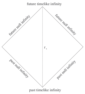
Figure 1: Penrose diagram for the asymptotically flat wormhole spacetime considered in this work.

Throughout this work we consider the specific case of a constant redshift function, i.e., $\Phi^{\prime}=0$, and taking into account the shape function given by Eq. (14), the stress-energy tensor components take the following form

$$\rho(r) =\frac{r_{S}}{(2\pi\alpha)^{3/2}}\;\mathrm{exp}\left(-\frac{r^{2}}{4\alpha}\right)\,,$$ (16)

$$p_{r}(r) =-\frac{r_{S}}{4\pi^{3/2}r^{3}}\;\gamma\left(\frac{3}{2},\frac{r^{2}}{4\alpha}\right)$$ (17)

$$p_{t}(r) =-\frac{r_{S}}{8\pi^{3/2}r^{3}}\Bigg{[}\frac{r^{3}}{4\alpha^{3/2}}\;\mathrm{exp}\left(-\frac{r^{2}}{4\alpha}\right)-\gamma\left(\frac{3}{2},\frac{r^{2}}{4\alpha}\right)\Bigg{]}$$ (18)

There are some necessary ingredients to be a wormhole solution. First of all, the existence of a throat expressed by the condition $b(r_{0})=r_{0}$, namely

$$\frac{1}{a}\gamma\left(\frac{3}{2},x_{0}^{2}\right)=x_{0},$$ (19)

where we have defined

$$x_{0}=\frac{r_{0}}{2\sqrt{\alpha}}\qquad\text{and}\qquad a=\frac{\sqrt{\alpha\pi}}{r_{S}}\,,$$ (20)

for notational simplicity.

In order to have one and only one solution we search for extrema of

$$\frac{1}{x_{0}}\gamma\left(\frac{3}{2},x_{0}^{2}\right)=a\,,$$ (21)

which provides

$$\bar{x}_{0}=1.5112=\frac{\bar{r}_{0}}{2\sqrt{\alpha}}\,,\quad\text{and}\quad\frac{1}{\bar{x}_{0}}\gamma\left(\frac{3}{2},\bar{x}_{0}^{2}\right)=0.4654\,.$$ (22)

From these relationships we deduce that

$$\frac{\sqrt{\alpha\pi}}{r_{S}}=0.4654=a\,,$$ (23)

or

$$3.81\sqrt{\alpha}=r_{\alpha}=r_{S}\,,$$ (24)

which finally provides a relationship between $r_{0}$ and $r_{S}$ given by

$$r_{S}=\bar{r}_{0}\frac{\sqrt{\pi}}{2\bar{x}_{0}a}=1.2599\bar{r}_{0}.$$ (25)

Note that three cases, represented in Fig. 2, need to be analyzed:

a)

If $r_{\alpha}>r_{S}$, we have no solutions and therefore no throats;

b)

If $r_{\alpha}<r_{S}$, we have two solutions denoting an inner throat $r_{-}$ and an outer throat $r_{+}$ with $r_{+}>r_{-}$.

c)

If $r_{\alpha}=r_{S}$, we find the value of Eq. $\left(\ref{x0}\right)$. This corresponds to the situation when $r_{+}=r_{-}$ and it will be interpreted as an “extreme ” situation like the extreme Reissner-Nordström metric.

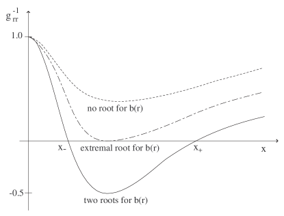
Figure 2: Plot of $g_{rr}^{-1}$ as a function of $x=r/\left(2\sqrt{\alpha}\right)$ for three different situations: a) no root, b) extremal root and c) two roots $x_{+}=r_{+}/\left(2\sqrt{\alpha}\right)$ and $x_{-}=r_{-}/\left(2\sqrt{\alpha}\right)$. See the text for details.

Unfortunately, case c) does not satisfy the flaring out condition $b^{\prime}(r_{0})<1$ and therefore will be discarded. We fix our attention to case b), which satisfies the flaring out condition. Note that we necessarily have $r_{+}>\bar{r}_{0}\simeq 3\sqrt{\alpha}$. Since the throat location depends on the value of $a$, we can set without a loss of generality $r_{+}=k\sqrt{\alpha}$ with $k>3$. Therefore

$$b\left(r_{+}\right)=r_{+}=k\sqrt{\alpha}=\frac{2r_{S}}{\sqrt{\pi}}\gamma\left(\frac{3}{2},\frac{k^{2}}{4}\right).$$ (26)

To avoid the region $r_{-}\leq r\leq r_{+}$ in which $(1-b(r)/r)<0$, we define the range of $r$ to be $r_{+}\leq r<\infty$. In the analysis below, we require the form of $b^{\prime}(r_{+})$ and $b^{\prime\prime}(r_{+})$. Thus, by defining

$$x=\frac{r_{+}}{2\sqrt{\alpha}},$$ (27)

we deduce the following useful relationships

$$b^{\prime}\left(r_{+}\right) =\frac{r_{S}r_{+}^{2}}{2\sqrt{\pi\alpha^{3}}}\exp\left(-\frac{r_{+}^{2}}{4\alpha}\right)$$

$$=\frac{2x^{3}}{\gamma\left(\frac{3}{2},x^{2}\right)}\exp\left(-x^{2}\right)$$ (28)

and

$$b^{\prime\prime}\left(r_{+}\right) =\frac{2r_{S}}{\sqrt{\pi}}\exp\left(-\frac{r_{+}^{2}}{4\alpha}\right)\frac{r_{+}}{2\sqrt{\alpha^{3}}}\left[1-\frac{r_{+}^{2}}{4\alpha}\right]$$

$$=\frac{2x^{2}}{\sqrt{\alpha}\gamma\left(\frac{3}{2},x^{2}\right)}\exp\left(-x^{2}\right)\left(1-x^{2}\right)\,,$$ (29)

respectively.

The behavior of $b^{\prime}(r_{+})$ and $b^{\prime\prime}(r_{+})$ are depicted in Fig. 3 for convenience. An extremely interesting case is that of $b^{\prime}(r_{+})$ $\ll 1$, which is valid in the range $r_{+}\gtrsim 6\sqrt{\alpha}$ (or $x\gtrsim 3$), as is transparent from the plots in Fig. 3. This will be explored in detail below. Note also that $\sqrt{\alpha}b^{\prime\prime}(r_{+})\ll 1$ for $x\gtrsim 3$.

Figure 3: Plots of $b^{\prime}(r_{+})$ and $\sqrt{\alpha}b^{\prime\prime}(r_{+})$. Note that $b^{\prime}\ll 1$ for $x\gtrsim 3$. This characteristic is analyzed in detail below, in finding wormhole specific wormhole solutions.

III Self-sustained wormholes in noncommutative geometry

In this section, we consider a semi-classical analysis, where the Einstein field equation takes the form

$$G_{\mu\nu}=\kappa\,\langle T_{\mu\nu}\rangle^{\mathrm{ren}}\,,$$ (30)

with $\kappa=8\pi G$, and $\langle T_{\mu\nu}\rangle^{\mathrm{ren}}$ is the renormalized expectation value of the stress-energy tensor operator of the quantized field. Now, the metric may be separated into a background component, $\bar{g}_{\mu\nu}$ and a perturbation $h_{\mu\nu}$, i.e., $g_{\mu\nu}=\bar{g}_{\mu\nu}+h_{\mu\nu}$. The Einstein tensor may also be separated into a part describing the curvature due to the background geometry and that due to the perturbation, i.e.,

$$G_{\mu\nu}(g_{\alpha\beta})=G_{\mu\nu}(\bar{g}_{\alpha\beta})+\Delta G_{\mu\nu}(\bar{g}_{\alpha\beta},h_{\alpha\beta})\,,$$ (31)

where $\Delta G_{\mu\nu}(\bar{g}_{\alpha\beta},h_{\alpha\beta})$ may be considered a perturbation series in terms of $h_{\mu\nu}$. Using the semi-classical Einstein field equation, in the absence of matter fields, one may define an effective stress-energy tensor for the quantum fluctuations as

$$\langle T_{\mu\nu}\rangle^{\mathrm{ren}}=-\frac{1}{\kappa}\,\langle\Delta G_{\mu\nu}(\bar{g}_{\alpha\beta})\rangle^{\mathrm{ren}}\,,$$ (32)

so that the equation governing quantum fluctuations behaves as a backreaction equation. The semi-classical procedure followed in this work relies heavily on the formalism outlined in Refs. Garattini ; Garattini:2007ff , where the graviton one loop contribution to a classical energy in a traversable wormhole background was computed, through a variational approach with Gaussian trial wave functionals Garattini ; Garattini2 . A zeta function regularization is used to deal with the divergences, and a renormalization procedure is introduced, where the finite one loop is considered as a self-consistent source for traversable wormholes. Rather than reproduce the formalism, we shall refer the reader to Refs. Garattini ; Garattini:2007ff for details, when necessary. In this paper, rather than integrate over the whole space as in Ref. Garattini , we shall work with the energy densities, which provides a more general working hypothesis, which follows the approach outlined in Ref. Garattini:2007ff . However, for self-completeness and self-consistency, we present here a brief outline of the formalism used.

The classical energy is given by

$$H_{\Sigma}^{(0)}=\int_{\Sigma}\,d^{3}x\,\mathcal{H}^{(0)}=-\frac{1}{16\pi G}\int_{\Sigma}\,d^{3}x\,\sqrt{g}\,R\,,$$ (33)

where the background field super-hamiltonian, $\mathcal{H}^{(0)}$, is integrated on a constant time hypersurface. $R$ is the curvature scalar given by Eq. $\left(\ref{Ricciscalar}\right)$, and for simplicity we consider $\Phi^{\prime}=0$, as mentioned above, which provides interesting enough results. Thus, the classical energy reduces to

$$H_{\Sigma}^{(0)}=-\frac{1}{2G}\int_{r_{0}}^{\infty}\,\frac{dr\,r^{2}}{\sqrt{1-b(r)/r}}\,\frac{b^{\prime}(r)}{r^{2}}\,.$$ (34)

We shall also take into account the total regularized one loop energy given by

$$E^{TT}=2\int_{r_{0}}^{\infty}\,dr\frac{r^{2}}{\sqrt{1-b(r)/r}}\,\left[\rho_{1}(\varepsilon,\mu)+\rho_{2}(\varepsilon,\mu)\right]\,,$$ (35)

where once again, we refer the reader to Refs. Garattini ; Garattini:2007ff for details. The energy densities, $\rho_{i}(\varepsilon)$ (with $i=1,2$), are defined as

$$\rho_{i}(\varepsilon,\mu) =\frac{1}{4\pi}\mu^{2\varepsilon}\int_{\sqrt{U_{i}(r)}}^{\infty}\,d\tilde{E}_{i}\,\frac{\tilde{E}_{i}^{2}}{\left[\tilde{E}_{i}^{2}-U_{i}(r)\right]^{\varepsilon-1/2}}$$

$$=-\frac{U_{i}^{2}(r)}{64\pi^{2}}\left[\frac{1}{\varepsilon}+\ln\left(\frac{\mu^{2}}{U_{i}}\right)+2\ln 2-\frac{1}{2}\right].$$ (36)

The zeta function regularization method has been used to determine the energy densities, $\rho_{i}$. It is interesting to note that this method is identical to the subtraction procedure of the Casimir energy computation, where the zero point energy in different backgrounds with the same asymptotic properties is involved (see also Ref. DGL for a related issue in the context of topology change). In this context, the additional mass parameter $\mu$ has been introduced to restore the correct dimension for the regularized quantities. Note that this arbitrary mass scale appears in any regularization scheme.

We emphasize that in analyzing the Einstein field equations, one should consider the whole system of equations, which in the static spherically symmetric case also includes the $rr$-component. The joint analysis of the equations is necessary to guarantee the compatibility of the system. However, in the semi-classical framework considered in this work there is no dynamical equation for the pressure. Nevertheless, one may argue that the semi-classical part of the pressure is known through the equation of state that determines the relation between the energy density and the pressure.

Since a self sustained wormhole must satisfy

$$H_{\Sigma}^{(0)}=-\,E^{TT},$$ (37)

which is an integral relation, this has to be true also for the integrand, namely the energy density. Therefore, we set

$$\frac{b^{\prime}(r)}{2Gr^{2}}=2\,\left[\rho_{1}(\varepsilon,\mu)+\rho_{2}(\varepsilon,\mu)\right]\,.$$ (38)

For this purpose, the Lichnerowicz equations provide the potentials, which are given by

$$U_{1}(r)=\frac{6}{r^{2}}\,\left[1-\frac{b(r)}{r}\right]-\frac{3}{2r^{2}}\,\left[b^{\prime}(r)-\frac{b(r)}{r}\right]\,,$$ (39)

$$U_{2}(r)=\frac{6}{r^{2}}\,\left[1-\frac{b(r)}{r}\right]-\frac{3}{2r^{2}}\,\left[\frac{b^{\prime}(r)}{3}+\frac{b(r)}{r}\right].$$ (40)

We refer the reader to Refs. Garattini ; Garattini:2007ff for the deduction of these expressions. Thus, taking into account Eq. $\left(\ref{energy}\right)$, then Eq. $\left(\ref{Ett}\right)$ yields the following relationship

$$\frac{b^{\prime}(r)}{2Gr^{2}} =-\frac{1}{32\pi^{2}\varepsilon}\,\left[U_{1}^{2}(r)+U_{2}^{2}(r)\right]$$

$$-\frac{1}{32\pi^{2}}\left[U_{1}^{2}\ln\left(\left|\frac{4\mu^{2}}{U_{1}\sqrt{e}}\right|\right)+U_{2}^{2}\ln\left(\left|\frac{4\mu^{2}}{U_{2}\sqrt{e}}\right|\right)\right].$$ (41)

It is essential to renormalize the divergent energy by absorbing the singularity in the classical quantity, by redefining the bare classical constant $G$ as

$$\frac{1}{G}\rightarrow\frac{1}{G_{0}}-\frac{2}{\varepsilon}\,\frac{\left[U_{1}^{2}(r)+U_{2}^{2}(r)\right]}{32\pi^{2}}\frac{r^{2}}{b^{\prime}(r)}\,.$$ (42)

Using this, Eq. $\left(\ref{selfsust}\right)$ takes the form

$$\,\frac{b^{\prime}(r)}{2G_{0}r^{2}}=-\frac{1}{32\pi^{2}}\left[U_{1}^{2}\ln\left(\left|\frac{4\mu^{2}}{U_{1}\sqrt{e}}\right|\right)+U_{2}^{2}\ln\left(\left|\frac{4\mu^{2}}{U_{2}\sqrt{e}}\right|\right)\right].$$ (43)

Note that this quantity depends on an arbitrary mass scale. Thus, using the renormalization group equation to eliminate this dependence, we impose that

$$\mu\frac{d}{d\mu}\left[\frac{b^{\prime}(r)}{2G_{0}\left(\mu\right)r^{2}}\right] =-\frac{\mu}{32\pi^{2}}\frac{d}{d\mu}\Bigg{[}U_{1}^{2}\ln\left(\left|\frac{4\mu^{2}}{U_{1}\sqrt{e}}\right|\right)$$

$$+U_{2}^{2}\ln\left(\left|\frac{4\mu^{2}}{U_{2}\sqrt{e}}\right|\right)\Bigg{]}\,,$$ (44)

which reduces to

$$\frac{b^{\prime}(r)}{r^{2}}\,\mu\,\frac{\partial G_{0}^{-1}(\mu)}{\partial\mu}=-\frac{1}{8\pi^{2}}\,\left[U_{1}^{2}(r)+U_{2}^{2}(r)\right]\,.$$ (45)

The renormalized constant $G_{0}$ is treated as a running constant, in the sense that it varies provided that the scale $\mu$ is varying, so that one may consider the following definition

$$\frac{1}{G_{0}(\mu)}=\frac{1}{G_{0}(\mu_{0})}-\frac{\left[U_{1}^{2}(r)+U_{2}^{2}(r)\right]}{8\pi^{2}}\,\,\frac{r^{2}}{b^{\prime}(r)}\,\ln\left(\frac{\mu}{\mu_{0}}\right)\,,$$ (46)

which can be cast into the following form

$$G_{0}(\mu)=\frac{G_{0}(\mu_{0})}{1-G_{0}(\mu_{0})a\left(r\right)\ln\left(\frac{\mu}{\mu_{0}}\right)},$$ (47)

where

$$a\left(r\right)=\frac{\left[U_{1}^{2}(r)+U_{2}^{2}(r)\right]}{8\pi^{2}}\,\,\frac{r^{2}}{b^{\prime}(r)}.$$ (48)

We can note that there is a blow up at a scale

$$\mu_{0}\exp\left(\frac{1}{G_{0}(\mu_{0})a\left(r\right)}\right)=\mu,$$ (49)

which is very large if the argument of the exponential is large. This is called a Landau point invalidating the perturbative computation. Thus, Eq. $\left(\ref{selfsust}\right)$ finally provides us with

$$\frac{16\pi^{2}}{G_{0}(\mu_{0})} =-\frac{r^{2}}{b^{\prime}(r)}\,\Bigg{[}U_{1}^{2}(r)\ln\left(\left|\frac{4\mu_{0}^{2}}{U_{1}(r)\sqrt{e}}\right|\right)$$

$$+U_{2}^{2}(r)\ln\left(\left|\frac{4\mu_{0}^{2}}{U_{2}(r)\sqrt{e}}\right|\right)\Bigg{]}.$$ (50)

Now, the procedure that we shall follow is to find the extremum of the right hand side of Eq. $\left(\ref{selfsust4}\right)$ with respect to $r$, and finally evaluate at the throat $r_{0}$, in order to have only one solution (see discussion in Ref. Garattini ).

To this effect, we shall use the derivative of the potentials, Eqs. $\left(\ref{p1}\right)$-$\left(\ref{p2}\right)$, which we write down for self-completeness and self-consistency, and are given by

$$U_{1}^{\prime}(r) = -\frac{12}{r^{3}}\left(1-\frac{b}{r}\right)+\frac{6(b-b^{\prime}r)}{r^{4}}$$ (51)

$$-\frac{3}{2r^{2}}\left[b^{\prime\prime}-\frac{b^{\prime}r-b}{r^{2}}\,\right],$$

$$U_{2}^{\prime}(r) = -\frac{12}{r^{3}}\left(1-\frac{b}{r}\right)+\frac{6(b-b^{\prime}r)}{r^{4}}$$ (52)

$$-\frac{3}{2r^{2}}\left[\frac{b^{\prime\prime}}{3}+\frac{b^{\prime}r-b}{r^{2}}\right],$$

and once evaluated at the throat take the following form

$$U_{1}^{\prime}(r_{+}) =\frac{9(1-b^{\prime}\left(r_{+}\right))}{2r_{+}^{3}}-\frac{3b^{\prime\prime}\left(r_{+}\right)}{2r_{+}^{2}}\,,$$ (53)

$$U_{2}^{\prime}(r_{+}) =\frac{15(1-b^{\prime}\left(r_{+}\right))}{2r_{+}^{3}}-\frac{b^{\prime\prime}\left(r_{+}\right)}{2r_{+}^{2}}\,,$$ (54)

respectively. The potentials, Eqs. $\left(\ref{p1}\right)$-$\left(\ref{p2}\right)$ evaluated at the throat reduce to

$$U_{1}(r_{+}) =-\frac{3}{2r_{+}^{2}}\left[b^{\prime}(r_{+})-1\right]\,,$$ (55)

$$U_{2}(r_{+}) =-\frac{3}{2r_{+}^{2}}\,\left[\frac{b^{\prime}(r_{+})}{3}+1\right]\,.$$ (56)

Thus, the extremum of Eq. $\left(\ref{selfsust4}\right)$ with respect to $r$, takes the form

$$\frac{r}{2\alpha}\,\left[U_{1}^{2}\ln\left(\frac{|U_{1}|\sqrt{e}}{4\mu_{0}^{2}}\right)+U_{2}^{2}\ln\left(\frac{|U_{2}|\sqrt{e}}{4\mu_{0}^{2}}\right)\right]$$

$$+\left[2U_{1}U_{1}^{\prime}\ln\left(\frac{|U_{1}|e}{4\mu_{0}^{2}}\right)+2U_{2}U_{2}^{\prime}\ln\left(\frac{|U_{2}|e}{4\mu_{0}^{2}}\right)\right]=0,$$ (57)

where the following relationship

$$\left[U_{i}^{2}\ln\left(\frac{|U_{i}|\sqrt{e}}{4\mu_{0}^{2}}\right)\right]^{\prime}=2U_{i}U_{i}^{\prime}\ln\left(\frac{|U_{i}|e}{4\mu_{0}^{2}}\right),$$ (58)

has been used.

Considering the general features given by Eqs. (28) and (29) provides an intractable analysis to the problem. However, an extremely interesting case which we explore in detail is that of $b^{\prime}(r_{+})$ $\ll 1$, which is justified for the range $r_{+}\gtrsim 6\sqrt{\alpha}$ (or $x\gtrsim 3$), as is transparent from the plots in Fig. 3. Thus, the potentials, Eqs. $\left(\ref{p1}\right)$-$\left(\ref{p2}\right)$ evaluated at the throat reduce to

$$U_{1}(r_{+}) \simeq\frac{3}{2r_{+}^{2}}\,,$$ (59)

$$U_{2}(r_{+}) \simeq-\frac{3}{2r_{+}^{2}}\,,$$ (60)

respectively. The derivatives of the potentials $U_{1}(r_{+})$ and $U_{2}(r_{+})$ at the throat, Eqs. $\left(\ref{p01}\right)$-$\left(\ref{p02}\right)$, take the following form

$$U_{1}^{\prime}(r_{+}) \simeq\frac{9}{2r_{+}^{3}}-\frac{3b^{\prime\prime}\left(r_{+}\right)}{2r_{+}^{2}}\,,$$ (61)

$$U_{2}^{\prime}(r_{+}) \simeq\frac{15}{2r_{+}^{3}}-\frac{b^{\prime\prime}\left(r_{+}\right)}{2r_{+}^{2}}\,.$$ (62)

Finally, we verify that Eq. $\left(\ref{Ap2}\right)$ provides

$$\frac{3}{4\alpha}\ln\left(\frac{3\sqrt{e}}{8\mu_{0}^{2}r_{+}^{2}}\right)-\left[\frac{6}{r_{+}^{2}}+\frac{b^{\prime\prime}(r_{+})}{r_{+}}\right]\ln\left(\frac{3e}{8\mu_{0}^{2}r_{+}^{2}}\right)=0.$$ (63)

Note that the factor in square brackets in the second term may be expressed as

$$\left[\frac{6}{r_{+}^{2}}+\frac{b^{\prime\prime}(r_{+})}{r_{+}}\right]=\frac{6}{r_{+}^{2}}\left[1+\frac{1}{6}r_{+}b^{\prime\prime}(r_{+})\right]\,,$$ (64)

and using the following dimensionless relationship

$$r_{+}b^{\prime\prime}(r_{+})=\frac{4x^{3}}{\gamma\left(\frac{3}{2},x^{2}\right)}\exp\left(-x^{2}\right)\left(1-x^{2}\right)\,,$$ (65)

where $x$ is given by Eq. $\left(\ref{def:x}\right)$, one immediately verifies that $r_{+}b^{\prime\prime}(r_{+})\ll 1$ for $x\gtrsim 3$, which is transparent from Fig. 4.

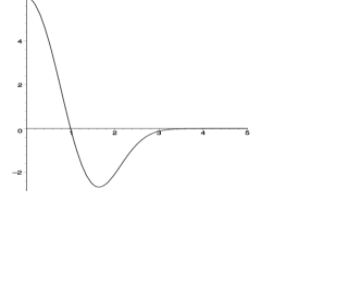
Figure 4: Plot depicting the behavior of $r_{+}b^{\prime\prime}(r_{+})$.

Thus, Eq. $\left(\ref{approx1}\right)$ reduces to

$$\ln\left(\frac{3\sqrt{e}}{8\mu_{0}^{2}r_{+}^{2}}\right)=\frac{8\alpha}{r_{+}^{2}}\ln\left(\frac{3e}{8\mu_{0}^{2}r_{+}^{2}}\right)\,,$$ (66)

which in turn may be reorganized to yield the following useful relationship

$$\left(1-\frac{8}{k^{2}}\right)\ln\left(\frac{3e}{8\mu_{0}^{2}\alpha k^{2}}\right)=\frac{1}{2},$$ (67)

where we have set, as defined in Eq. (26), $r_{+}=k\sqrt{\alpha}$, with $k>4$. Isolating the $k$-dependent term provides the expression

$$\frac{8\mu_{0}^{2}\alpha}{3\sqrt{e}}=\;k^{-2}\exp\left(-\frac{4}{k^{2}-8}\right)\,.$$ (68)

It is interesting to note that the r.h.s. has two extrema for positive $k$: $k_{1}=2$ and $k_{2}=4$. In terms of the wormhole throat the first value becomes $r_{1}=2\sqrt{\alpha}$, which will be discarded because its location is below the extreme radius, as emphasized in Section II.2. Relative to the second extrema $k_{2}$, i.e., $r_{2}=4\sqrt{\alpha}$, despite the fact that $k_{2}$ is larger than the extreme value $\left(k=3\right)$, it does not fall into the range of the approximation of $b^{\prime}\left(r_{+}\right)\ll 1$. Thus, it may also be discarded. Therefore, we need to search for values larger than $k=4$. In particular, according to Eq. $\left(\ref{bsec}\right)$, to neglect $r_{+}b^{\prime\prime}(r_{+})$ we must set $k\geq 6$. To this purpose, we build the following table

60.1220270.1069880.09484.fragments fragments60.1220270.1069880.09484\begin{tabular}[c]{|c|c|}\hline\cr Values of $k$&$\mu_{0}\sqrt{\alpha}$\\ \hline\cr$6$&$0.12202$\\ \hline\cr$7$&$0.10698$\\ \hline\cr$8$&$0.09484$\\ \hline\cr\end{tabular}\ \ \ \ .

Values of k μ0αValues of k μ0α (69)

Plugging the expression of $\mu_{0}\sqrt{\alpha}$, i.e., Eq. (68), into Eq.$\left(\ref{selfsust4}\right)$, we get

$$\frac{9\gamma\left(\frac{3}{2},\frac{k^{2}}{4}\right)}{2\pi^{2}k^{5}\left(k^{2}-8\right)}\exp\left(\frac{k^{2}}{4}\right)=\,\frac{\alpha}{G_{0}(\mu_{0})}.$$ (70)

The following table illustrates the behavior of $\sqrt{G_{0}(\mu_{0})/\alpha}$, and therefore of $r_{+}/\sqrt{G_{0}(\mu_{0})}$

60.122600.7470.350062. 5k¯=7.7777017.7777081.398831197.6417569.1056.236205. 6×102.fragments 60.122600.7470.350062.5fragments¯𝑘7.7777017.7777081.398831197.64175fragments69.fragments1056.23620fragments5.6102\begin{tabular}[c]{|c|c|c|}\hline\cr Values of $k$&$\sqrt{\alpha/G_{0}\left(\mu_{0}\right)}$&$r_{+}/\sqrt{G_{0}\left(\mu_{0}\right)}$\\ \hline\cr$6$&$0.12260\allowbreak$&$\allowbreak\allowbreak 0.74$\\ \hline\cr$7$&$0.35006$&$2.\,\allowbreak 5$\\ \hline\cr$\bar{k}=7.77770$&$1$&$\allowbreak\allowbreak 7.77770$\\ \hline\cr$8$&$1.39883$&$\allowbreak\allowbreak 11$\\ \hline\cr$9$&$7.64175$&$\allowbreak 69.$\\ \hline\cr$10$&$56.23620$&$\allowbreak 5.\,\allowbreak 6\times 10^{2}$\\ \hline\cr\end{tabular}\ \ \ \ .

Values of k /αG0(μ0)/r+G0(μ0)Values of k /αG0(μ0)/r+G0(μ0) (71)

Note that in table $\left(\ref{T1}\right)$, as $k$ increases then $\mu_{0}\sqrt{\alpha}$ decreases. This means that we are approaching the classical value where the non-commutative parameter $\alpha\rightarrow 0$. It appears also that there exists a critical value of $k$ where $\alpha=G_{0}\left(\mu_{0}\right)$. To fix ideas, suppose we fix $G_{0}\left(\mu_{0}\right)$ at the Planck scale, then below $\bar{k}$, the non-commutative parameter becomes more fundamental than $G_{0}\left(\mu_{0}\right)$. This could be a signal of another scale appearing, maybe connected with string theory. On the other hand above $\bar{k}$, we have the reverse. However, the increasing values in the table is far to be encouraging because the non commutative approach breaks down when $k$ is very large. Nevertheless, note the existence of interesting solutions in the neighborhood of the value $\bar{k}=7.7$.

IV Conclusion

In this work, we have analyzed exact wormhole solutions in the context of noncommutative geometry. The energy density of these wormhole geometries is a smeared and particle-like gravitational source, where the mass is diffused throughout a region of linear dimension $\sqrt{\alpha}$ due to the intrinsic uncertainty encoded in the coordinate commutator. The physical properties and characteristics of these wormhole solutions were further explored. Finally, we analyzed these wormhole geometries in semi-classical gravity, considering that the equation governing quantum fluctuations behaves as a backreaction equation. In particular, the energy density of the graviton one loop contribution to a classical energy in a traversable wormhole background and the finite one loop energy density is considered as a self-consistent source for these wormhole geometries. What we discover is that there exists a continuous set of solutions parametrized by $k$. Apparently, this set of solutions is unbounded for large values of $k$. However, as the critical value $\bar{k}$ is passed we note a vary rapidly divergent value of the ratio $\alpha/G_{0}\left(\mu_{0}\right)$ with a consequent growing of the wormhole radius. Nevertheless, this sector of the $k$-range does not represent physical solutions because we are approaching the region where $\alpha=0$. Moreover, from Eq. $\left(\ref{Landau}\right)$ we can see that the larger the value of $k$, the closer is the value of the scale $\mu$ to the Landau point or in other words, for large values of $k$ there is no evolution for the Eq. $\left(\ref{selfsust4}\right)$. This is evident by plugging in expression $\left(\ref{rad2b}\right)$ into Eq. $\left(\ref{selfsust4a}\right)$ leading to

$$\mu_{0}\exp\left(\frac{2\alpha}{r^{2}-8\alpha}\right)=\mu_{0}\exp\left(\frac{2}{k^{2}-8}\right)=\mu.$$ (72)

On the other hand, within the range of validity of the approximation where $b^{\prime}(r_{+})$ $\ll 1$, we find that we are far from the blow up region which means that the perturbative computation in this range can be considered correct.

References

- (1) E. Witten, Nucl. Phys. B 460, 335 (1996) [arXiv:hep-th/9510135]; N. Seiberg and E. Witten, JHEP 9909, 032 (1999) [arXiv:hep-th/9908142].
- (2) A. Smailagic and E. Spallucci, J. Phys. A 36, L467 (2003) [arXiv:hep-th/0307217].
- (3) P. Nicolini, A. Smailagic and E. Spallucci, Phys. Lett. B 632, 547 (2006) [arXiv:gr-qc/0510112].
- (4) E. Di Grezia, G. Esposito and G. Miele, J.Phys.A 41, 164063 (2008) [arXiv:0707.3318 [gr-qc]].
- (5) R. Casadio and P. Nicolini, arXiv:0809.2471 [hep-th]; P. Nicolini, arXiv:0807.1939 [hep-th]; E. Spallucci, A. Smailagic and P. Nicolini, arXiv:0801.3519 [hep-th]; S. Ansoldi, P. Nicolini, A. Smailagic and E. Spallucci, Phys. Lett. B 645, 261 (2007); P. Nicolini, J. Phys. A 38, L631 (2005).
- (6) M. S. Morris and K. S. Thorne, Am. J. Phys. 56, 395 (1988).
- (7) H. G. Ellis, J. Math. Phys. 14 (1973) 104; K. A. Bronnikov, Acta Phys. Polon. B 4 (1973) 251.
- (8) B. Bhawal and S. Kar, Phys. Rev. D 46, 2464-2468 (1992); G. Dotti, J. Oliva, and R. Troncoso, Phys. Rev. D 75, 024002 (2007).
- (9) L. A. Anchordoqui and S. E. P Bergliaffa, Phys. Rev. D 62, 067502 (2000); K. A. Bronnikov and S.-W. Kim, Phys. Rev. D 67, 064027 (2003); M. La Camera, Phys. Lett. B573, 27-32 (2003); F. S. N. Lobo, Phys. Rev. D 75, 064027 (2007).
- (10) K. K. Nandi, B. Bhattacharjee, S. M. K. Alam and J. Evans, Phys. Rev. D 57, 823 (1998).
- (11) R. Garattini and F. S. N. Lobo, Class. Quant. Grav. 24, 2401 (2007).
- (12) C. G. Boehmer, T. Harko and F. S. N. Lobo, Phys. Rev. D 76, 084014 (2007); C. G. Boehmer, T. Harko and F. S. N. Lobo, Class. Quant. Grav. 25, 075016 (2008).
- (13) S. Sushkov, Phys. Rev. D 71, 043520 (2005); F. S. N. Lobo, Phys. Rev. D 71, 084011 (2005); F. S. N. Lobo, Phys. Rev. D 71, 124022 (2005); F. S. N. Lobo, Phys. Rev. D 73, 064028 (2006); F. S. N. Lobo, Phys. Rev. D 75, 024023 (2007).
- (14) F. S. N. Lobo, Class. Quant. Grav. 25, 175006 (2008).
- (15) J. P. S. Lemos, F. S. N. Lobo and S. Quinet de Oliveira, Phys. Rev. D 68, 064004 (2003).
- (16) F. S. N. Lobo, arXiv:0710.4474 [gr-qc].
- (17) S. V. Sushkov, Phys. Lett. A164, 33-37 (1992); A. A. Popov and S. V. Sushkov, Phys. Rev. D 63, 044017 (2001) [arXiv:gr-qc/0009028]; A. A. Popov, Phys. Rev. D 64, 104005 (2001) [arXiv:hep-th/0109166]; D. Hochberg, A. Popov and S. V. Sushkov, Phys. Rev. Lett. 78, 2050 (1997) [arXiv:gr-qc/9701064]; N. R. Khusnutdinov and S. V. Sushkov, Phys. Rev. D 65, 084028 (2002) [arXiv:hep-th/0202068]; A. R. Khabibullin, N. R. Khusnutdinov and S. V. Sushkov, Class. Quant. Grav. 23 627-634 (2006) [arXiv:hep-th/0510232]; N. R. Khusnutdinov, Phys. Rev. D 67, 124020 (2003) [arXiv:hep-th/0304176].
- (18) R. Garattini, Class. Quant. Grav. 22 1105-1118 (2005) [arXiv:gr-qc/0501105]; R. Garattini, Class. Quant. Grav. 24, 1189 (2007) [arXiv:gr-qc/0701019].
- (19) R. Garattini, Int. J. Mod. Phys. A 14 2905-2920 (1999) [arXiv:gr-qc/9805096]; R. Garattini, Phys. Rev. D 59 104019 (1999) [arXiv:hep-th/9902006].
- (20) A. DeBenedictis, R. Garattini and F. S. N. Lobo, Phys. Rev. D 78 104003 (2008) [arXiv:0808.0839 [gr-qc]].