Statistical properties of the final state in one-dimensional ballistic aggregation

Abstract

We investigate the long time behaviour of the one-dimensional ballistic aggregation model that represents a sticky gas of $N$ particles with random initial positions and velocities, moving deterministically, and forming aggregates when they collide. We obtain a closed formula for the stationary measure of the system which allows us to analyze some remarkable features of the final ‘fan’ state. In particular, we identify universal properties which are independent of the initial position and velocity distributions of the particles. We study cluster distributions and derive exact results for extreme value statistics (because of correlations these distributions do not belong to the Gumbel-Fréchet-Weibull universality classes). We also derive the energy distribution in the final state. This model generates dynamically many different scales and can be viewed as one of the simplest exactly solvable model of $N$-body dissipative dynamics.

I Introduction

The ballistic aggregation model is one of the simplest interacting particles processes of non-equilibrium statistical mechanics and as such has attracted a lot of attention in the past decades carnevale . This model represents a gas of $N$ unit-mass particles forming clusters through perfectly inelastic adhesive collisions. The motion of a particle between two collisions is deterministic and free (i.e. ballistic) and the total mass and momentum in a collision are conserved whereas the kinetic energy is dissipated. The stochasticity in this model is due only to the initial configuration which consists of single particles randomly located with uncorrelated random velocities drawn from a continuous distribution. This dissipative system, usually referred to as ballistic aggregation or sticky gas, appears as a minimal model of cluster formation and provides a relevant statistical description of the merger of coherent structures such as vortices, thermal plumes, flowing granular media granular gas or the accumulation of cosmic dust into planetoids. The ballistic aggregation model also plays a role in the study of the large-scale structure of the universe because the motion of self-gravitating matter in the expanding universe is similar to that of matter moving solely by inertia Shandarin ; martin . Another noteworthy feature of this model stems from its connection with the Burgers equation, an important toy model in the study of turbulence: it can be shown that at very high Reynolds number, the solution of the Burgers equation in the long time limit consists of a series of shocks which follow exactly the dynamics of the ballistic aggregation model burgers ; kida ; frisch .

Ballistic aggregation exhibits at long time $t$ a self-similar coarsening behaviour first studied by Carnevale, Pomeau and Young carnevale . In one dimension, the coarsening regime occurs for intermediate times satisfying $t\sim N^{3/2}$, $N$ being the total mass or equivalently the total number of initial particles in the system. For longer times, and in the absence of any boundary, the system ultimately reaches a state where no more collisions are possible: the particles are grouped into clusters of different sizes (or masses) with velocities increasing from left to right. This final ordered state will be called the “fan” state. Once this state is reached, there is no further loss of energy and the system becomes stationary.

The aim of this paper is to investigate the properties of this fan state. We find an exact analytic formula for the joint probability distribution of the sizes and velocities of the clusters by mapping the final state of the ballistic aggregation model to the convex minorant of a one-dimensional random walk. From this invariant measure that fully characterizes the set of all possible fan states, various statistical properties of the model in the long time limit will be derived. In particular, we shall retrieve the known fact shida ; sibuya ; hyuga that the probability of obtaining a fan state with exactly $k$ clusters is a purely combinatorial factor (which is universal in the sense that it does not depend upon the initial velocity distribution of the particles). We shall prove that the cluster distribution in the fan state is identical to the statistics of cycles in a random permutation of $N$ objects goncharov ; shepp , both problems having a common underlying combinatorial structure related to the convex minorant construction spitzer ; steele . This will allow us to characterize the different scales that are dynamically generated in the system: in the large $N$ limit, the size of a typical cluster is of order $N/\ln N$, the largest cluster contains a finite fraction of the total mass $N$ and hence grows linearly with $N$, the smallest cluster scales as $\ln N$, and the rightmost cluster, which has the leading velocity, has a size of order $\sqrt{N}$. We shall also derive the (non-universal) joint distribution of mass and velocity of this ‘leader’ which is very different from the usual extreme-value distributions obtained for uncorrelated random variables. Finally, we shall show that the energy remaining in the system after all collisions have ended is of the order $\ln N$ and shall calculate the distribution of the scaling variable $E/\ln N$.

The paper is organized as follows. In Section-II we define the ballistic aggregation model and focus on its final fan state. In particular, we show how the statistical properties in the fan state are related to those of the convex minorant of an associated one dimensional random walk problem. This mapping allows us to derive explicitly the joint distribution of the cluster sizes and their velocities in the fan state which is one of the key results of this paper. In Section-III we show how this joint distribution can be used to derive the cluster size distribution in the fan state which turns out to be universal (with respect to the initial velocity distribution). This universal property is shown to be related to the statistics of cycles lengths in a random permutation problem. In Section-IV, we further exploit the joint distribution to compute exact asymptotic results for certain extreme variables in the fan state such as the size and the velocity distribution of the rightmost (‘leader’) cluster. In Section-V, we derive the exact asymptotic distribution of energy in the fan state. Finally we conclude in Section-VI with a summary and some open problems.

II Statistical Description of the Stationary State

II.1 Definition of the Model

The ballistic aggregation problem in one dimension is an elementary interactive particles process, the dynamics of which is defined as follows. At the initial time $t=0$, we start with $N$ particles randomly located on an infinite line. We label the particles as $i=1,2,\dotsc,N$ according to the order of their initial positions from left to right (see Fig. 1 where we have taken $N=6$). We denote by $v_{i}$ and $m_{i}$, respectively, the initial velocity and the mass of the $i$-th particle. For $t>0$, each particle moves ballistically at constant speed. When two particles meet they coalesce and form a single new particle whose mass is the sum of the initial masses and whose momentum is the sum of the initial momenta. The only randomness in the model lies in the initial conditions, i.e. the initial positions and velocities of each particle. We shall assume that the initial velocities $\{v_{i}\}$’s are uncorrelated random variables, drawn from a common continuous probability density function (PDF) $\phi(v)$. For simplicity, we assume that all the initial masses are the same and take them to be unity. Once the initial conditions are given, the evolution of a given realization is deterministic and fully determined by the mass and momentum conservation laws. The shocks being totally inelastic, energy is dissipated at each collision.

At late times $t\gg O(1)$ (but before the system feels the finiteness of the mass $N$), the ballistic aggregation model exhibits a coarsening regime where typical cluster size grows with time as a power law, as studied first by Carnevale, Pomeau and Young carnevale using scaling arguments and numerical simulations. For example, in this regime, the average size (or mass) of a particle-cluster grows as $t^{2D/(2+D)}$ and its velocity decreases as $t^{-D/(2+D)}$, $D$ being the spatial dimension. The global mass of the system being conserved, the total energy of the system decays as $t^{-2D/(2+D)}$. These exponents derived in   carnevale turn out to be correct in one dimension where the problem is exactly solvable martin ; frachebourg ; fracheb2 . This, however, turns out to be a bit fortuitous. In higher dimensions, the exponents predicted in  carnevale turn out to be incorrect due to strong correlations between the velocities of the colliding clusters at late times PaulK . In one dimension, it is possible to calculate exactly (in one dimension) the mass distribution of the clusters martin ; frachebourg ; fracheb2 in the scaling limit when $N\to\infty$ ($N$ being the total mass of the system) and $t\to\infty$, keeping the ratio $t/N^{3/2}$ finite martin ; frachebourg ; fracheb2 . However, these scaling results for the coarsening regime are valid only for intermediate times satisfying $t\sim N^{3/2}$. When $t\gg N^{3/2}$, the system evolves into a stationary state in which no more collisions can occur: the particles are grouped in $k$ disjoint clusters of different masses, where $k$ itself is a stochastic variable. Each cluster moves at a constant velocity, and the speed of a given cluster is larger than that of its left neighbour (if any) and less than that of its right neighbour (if any). In this ultimate state the clusters keep on moving farther apart, i.e., they fan out from each other with increasing time, thus justifying the name “fan” state (see Fig. 1). Once this fan state is reached, there is no further collision and hence no further dissipation of energy.

Figure 1: An example of a configuration of $6$ particles with identical initial mass $m_{i}=1$ and varying initial velocities, evolving in the long time limit into the fan state: the velocities are now increasing from left to right and there are no more colllisions.

In this work, we shall focus on the statistical description of the fan state of the random aggregation process. We shall show that properties of the fan state related to the sizes of the clusters (regardless of their respective ordering and their velocities) are universal as they do not depend on the PDF $\phi(v)$ from which the initial velocities of the particles are drawn. The cluster statistics can in fact be mapped to the cycle length distribution in random permutations, which are fundamental combinatorial objects. From this observation the distribution of the cluster masses and in particular the typical mass of the largest and the smallest cluster can readily be calculated. When the distribution of the velocities of the clusters is taken into account, universality with respect to $\phi(v)$ is lost. However, in the large $N$ limit, we will see that some universality is restored, thanks to the central limit theorem, in the size distribution of the rightmost cluster (the leader) provided the second moment $\sigma^{2}=\int_{-\infty}^{\infty}v^{2}\,\phi(v)\,dv$ is finite. Finally, we are also able to calculate explicitly the energy distribution in the fan state, but only for the special case when $\phi(v)$ is Gaussian.

II.2 The Fan State as a Convex Minorant

The fan state of the random aggregation process can be determined geometrically from the initial conditions sibuya . We now explain this graphical interpretation of the fan state as a convex minorant of a random walk. Recall that we label the particles as $i=1,2,\dotsc,N$ according to the order of their initial positions from left to right (see Fig. 1) and that we denote by $v_{i}$ respectively the initial velocity of the $i$-th particle (all the initial masses being unity). For any realization of the initial state $\{v_{1},v_{2},\ldots,v_{N}\}$, the final state is uniquely determined i.e. the number of final clusters, their masses and their velocities are unique.

The initial state $\{v_{1},v_{2},\ldots,v_{N}\}$ of the system is represented by a broken graph $(P_{0},P_{1},\ldots,P_{N})$ (see Fig. 2) such that:

(i) $P_{0}=(0,0)$ is the origin;

(ii) the coordinates of $P_{i}$ are given recursively by $P_{i}=P_{i-1}+(1,v_{i})$ for $1\leq i\leq N$.

In other words, the speed $v_{i}$ of the $i$-th particle is represented by the slope of the line $(P_{i-1}P_{i})$. We also emphasize that the horizontal coordinate of $P_{i}$ does not correspond to the actual position of the $i$-th particle but only on its label.

More generally, if we had started with particles having different masses $\{m_{1},m_{2},\ldots,m_{N}\}$ the coordinates of $P_{i}$ would be $P_{i}=P_{i-1}+m_{i}(1,v_{i})$ sibuya . In other words, the initial state is drawn as a random walk in the cumulative momentum and cumulative mass space as shown in Figs. 2 and 3.

Suppose that the first collision occurs between particles $i$ and $(i+1)$ with velocities $v_{i}$ and $v_{i+1}$ respectively. These two particles can aggregate if $v_{i}>v_{i+1}$, which means that the slope of the $(P_{i-1}P_{i})$ is larger than the slope of the $(P_{i}P_{i+1})$. Equivalently, this means that $P_{i}$ is located above the segment $(P_{i-1}P_{i+1})$ i.e., locally, the graph $(P_{i-1}P_{i}P_{i+1})$ has a negative curvature. After this collision, a cluster is formed with mass 2 and velocity $(v_{i}+v_{i+1})/2$. This cluster is represented by the vector $(P_{i-1}P_{i+1})$ (see Fig. 2) with coordinates $(2,v_{i}+v_{i+1}).$ We note that the slope of this vector again represents the velocity of the cluster. We now have a system of $N-1$ ‘particles’, with $N-2$ particles of mass 1 and one particle of mass 2. The state of this system is represented by a broken line in which the angle $(P_{i-1}P_{i}P_{i+1})$ with downward curvature is replaced by its base (see Fig. 2). Similarly, the next collision is also represented graphically by replacing another angle with downward curvature by its base (see Fig. 2) . This process will continue iteratively and the particles will aggregate forming clusters till all angles with downward curvature have been eliminated, i.e. all collisions have occurred. It follows that for any given initial state, the final state is uniquely given by the convex minorant of the corresponding random walk. Each line segment of the convex minorant represents a cluster in the fan state, —the horizontal and the vertical components of the segment give respectively the mass and the momentum of the cluster, i.e., the slope gives the velocity of the cluster. The geometry of the convex minorant (including the number of segments which represents the number of final clusters), however, differs from one realization of initial conditions to another. Various statistical properties of the ballistic aggregation in the fan state can be found from the statistical properties of the underlying convex minorant.

Figure 2: Initial configuration is represented by a graph (thin line) joining $P_{0}$ to $P_{N}$ (we have taken $m_{j}=1\;\forall j$). This graph can be interpreted as a random walk in the cumulative momentum and cumulative mass space. After the first collision the particles $i$ and $i+1$ aggregate into one cluster: in the associated graph, the angle $(P_{i-1}P_{i}P_{i+1})$ is replaced by the segment $(P_{i-1}P_{i+1})$.

Figure 3: We draw the convex minorant of the graph representing the same initial configuration as in Fig. 2. This convex minorant represents the final ‘fan’ state in which no more collisions can occur. Each straight segment of the convex minorant corresponds to a cluster of $n_{l}$ particles with momentum $n_{l}u_{l}$.

II.3 The Invariant Measure in the Fan State

We now derive the joint probability distribution which describes the fan state. Let $p_{N}(k;\{n_{i},u_{i}\})$ denote the joint PDF of having $k$ clusters in the fan state of masses and velocities $n_{i}$ and $u_{i}$ respectively, with $i=1,2,\dotsc,k$. Note that the various segments of the convex minorant (see Fig. 3) are correlated as their slopes must be increasingly ordered from left to right, i.e., $u_{1}<u_{2}<\dotsb<u_{k}$. Moreover, the total mass is conserved, $\sum_{i=1}^{k}n_{i}=N$. Once these two constraints are specified, the momentum of each final cluster is essentially determined by the conservation law:

$$n_{\ell}u_{\ell}=\sum_{j=N_{\ell-1}+1}^{N_{\ell}}m_{j}v_{j}$$ (1)

for the $\ell$-th cluster with $\ell=1,2,\dotsc,k$. We have defined here the cumulated masses $N_{k}=n_{1}+\ldots+n_{k}$. The sum in the above equation is thus restricted to the initial velocities of those particles which form the $\ell$-th cluster. We also recall that $m_{j}=1\;\forall j$. However, most importantly, to form a specific (say $\ell$-th) final cluster (i.e., a line segment in the underlying convex minorant) by aggregation of $n_{\ell}$ consecutive initial particles, the portion of the underlying random walk of $n_{\ell}$ steps must be such that it originates from one end of the line segment of convex minorant and finishes at its other end, while staying above the segment in the intermediate steps. Now, consider a random walk of $n_{\ell}$ steps that starts from one end of a line segment and finishes at its other end, but is otherwise allowed to cross the segment in the intermediate steps. For any realization of such a walk, given that there is one unique minimum with respect to the segment, if we consider all the $n_{\ell}$ cyclic permutations of the steps, then out of $n_{\ell}$ different realizations of the walks there is one and only one arrangement where in the intermediate steps the walk stays above the segment. This property is known as Raney’s lemma feller ; Knuth . (Here, the uniqueness of the arrangement is guaranteed by the fact that the PDF $\phi(v)$ is continuous).

Thus, the probability that a random walk of $n_{\ell}$ steps that starts at one end of a line segment and finishes at its other end while staying above the segment in-between equals $1/n_{\ell}$. Note that this probability is independent of the slope $u_{\ell}$ of the segment as well as the PDF $\phi(v)$ of the jump-lengths. Finally, gathering all the above inputs together we write

$$p_{N}(k;\{n_{i},u_{i}\}) =\delta\left(N-\sum_{i=1}^{k}n_{i}\right)\,\prod_{i=1}^{k-1}\theta(u_{i+1}-u_{i})$$

$$\times\prod_{\ell=1}^{k}\frac{1}{n_{\ell}}\left\langle\delta\left(u_{\ell}-\frac{1}{n_{\ell}}\sum_{j=N_{\ell-1}+1}^{N_{\ell}}v_{j}\right)\right\rangle,$$ (2)

where the angle brackets $\langle\dotsb\rangle$ denote the averaging over the set of initial velocities $\{v_{i}\}$. This key result provides a full statistical description of the clusters sizes and velocities in the fan state. From this joint probability distribution, all the statistical properties of the final state can be derived.

III Universal Statistical Properties of Clusters in the Fan State

In this section, we compute the distribution of the number and sizes of the clusters in the fan state: we will show that this distribution, obtained by integrating out the velocities of the clusters from the joint probability distribution given in Eq. (2), is universal with respect to the initial continuous PDF $\phi(v)$.

III.1 Statistics of the Total Number of Clusters in the Fan State

We first calculate $p_{N}(k)$, the probability that the final state contains $k$ distinct clusters. The value of $p_{N}(k)$ is obtained by summing Eq. (2) over all $n_{i}>0$’s and integrating it over $u_{i}$’s, keeping $k$ fixed. Thus,

$$p_{N}(k)=\sum_{\{n_{i}\}}\int\prod_{i=1}^{k}du_{i}\,\delta\left(N-\sum_{i=1}^{k}n_{i}\right)\,\prod_{i=1}^{k-1}\theta(u_{i+1}-u_{i})\prod_{\ell=1}^{k}\frac{{\mathcal{P}}(n_{\ell},u_{\ell})}{n_{\ell}}\,.$$ (3)

In this equation, we have used

$${\mathcal{P}}(n_{\ell},u_{\ell})=\left\langle\delta\left(u_{\ell}-\frac{1}{n_{\ell}}\sum_{j=N_{\ell-1}+1}^{N_{\ell}}v_{j}\right)\right\rangle=\int\,\delta\left(u_{\ell}-\frac{1}{n_{\ell}}\sum_{j=N_{\ell-1}+1}^{N_{\ell}}v_{j}\right)\prod_{j=N_{\ell-1}+1}^{N_{\ell}}\phi(v_{j})dv_{j}\,,$$ (4)

where $\phi$ is the distribution of the initial velocities. We note that the function ${\mathcal{P}}(n,u)$ is normalized:

$$\int_{-\infty}^{+\infty}du{\mathcal{P}}(n,u)=1\,.$$ (5)

To disentangle the constraints in Eq. (3), it is useful to consider the following generating function:

$$\sum_{N}p_{N}(k)z^{N}=\sum_{\{n_{i}\}}\frac{z^{n_{i}}}{n_{i}}\int\prod_{i=1}^{k}du_{i}\,\prod_{i=1}^{k-1}\theta(u_{i+1}-u_{i})\,\,{\mathcal{P}}(n_{i},u_{i})=\int\prod_{i=1}^{k}du_{i}\,\prod_{i=1}^{k-1}\theta(u_{i+1}-u_{i})\,\rho_{z}(u_{i})$$ (6)

with

$$\rho_{z}(u_{i})=\sum_{\{n_{i}\}}\frac{z^{n_{i}}}{n_{i}}{\mathcal{P}}(n_{i},u_{i})\,.$$ (7)

The integral on the right hand side (r.h.s) of Eq. (6) can be evaluated recursively and is found to be

$$\int_{-\infty}^{+\infty}du_{k}\rho_{z}(u_{k})\int_{-\infty}^{u_{k}}du_{k-1}\rho_{z}(u_{k-1})\ldots\int_{-\infty}^{u_{2}}du_{1}\rho_{z}(u_{1})=\frac{1}{k!}\Big{(}\int_{-\infty}^{+\infty}du_{k}\rho_{z}(u_{k})\Big{)}^{k}=\frac{1}{k!}\left(\sum_{\{n_{i}\}}\frac{z^{n_{i}}}{n_{i}}\right)^{k}\,,$$ (8)

where the last equality is obtained by using the definition of $\rho_{z}(u)$ in (7) and the normalization property in (5). Thus, for any given value of $k>0$, we have

$$\sum_{N}p_{N}(k)z^{N}=\frac{1}{k!}\Bigl{[}-\ln(1-z)\Bigr{]}^{k}\,.$$ (9)

After extracting the coefficient of $z^{N}$ on the r.h.s of this equation, we conclude that

$$p_{N}(k) =\frac{1}{k!}\sum_{\{n_{i}>1\}}^{\infty}\left[\prod_{i=1}^{k}n_{i}\right]^{-1}\delta\left(N-\sum_{i=1}^{k}n_{i}\right)\,.$$ (10)

This formula can be expressed in terms of some classical combinatorial numbers as follows. It is convenient to introduce a second auxiliary variable $t$ and to calculate the generating function of Eq. (9) with respect to $t$:

$$\sum_{k}\sum_{N}p_{N}(k)z^{N}t^{k}=\sum_{k}\frac{1}{k!}\Bigl{[}-\ln(1-z)\Bigr{]}^{k}t^{k}=(1-z)^{-t}=1+tz+\frac{t(t+1)}{2!}z^{2}+\frac{t(t+1)(t+2)}{3!}z^{3}+\ldots$$ (11)

Identifying the coefficients of $z^{N}$ on both sides of this equation we obtain the identity:

$$\sum_{k}p_{N}(k)t^{k}=\frac{t(t+1)(t+2)\ldots(t+N-1)}{N!}\,.$$ (12)

Using the classical formula

$$t(t+1)(t+2)\ldots(t+N-1)=\sum_{k=1}^{N}S_{1}(N,k)\,t^{k}\,,$$ (13)

that defines the unsigned Stirling numbers of the first kind riordan , $S_{1}(N,k)$, we conclude that the probability of finding $k$ clusters in the fan state for a system starting with $N$ distinct unit-mass particles is given by

$$p_{N}(k)= =\frac{S_{1}(N,k)}{N!},\quad\text{with}~{}k=1,2,\dotsc,N\,.$$ (14)

We thus recover by a different method the result of Ref. sibuya .

From Eq. (13), we observe that $\sum_{k=1}^{N}S_{1}(N,k)=N!$. Thus, $p_{N}(k)$, and consequently the joint PDF given by Eq. (2) are both clearly normalized as it must. Furthermore, using Eq. (12), one deduces that the mean number of clusters is given by $1+\frac{1}{2}+\ldots+\frac{1}{N}$.

In fact, it is well known riordan that the unsigned Stirling numbers $S_{1}(N,k)$ enumerate the number of permutations of $N$ elements with $k$ disjoint cycles exactly: thus, $p_{N}(k)$ is identical to the probability distribution of number of cycles in random permutations with uniform measure. Many results have been derived concerning the statistics of random permutations. For example, it has been shown in the context of permutation cycles shepp that for large $N$, $p_{N}(k)$ has a Gaussian form around its mean $\langle k\rangle\sim\ln N$, with a variance which is also of order $\ln N$. Therefore, the typical mass of a cluster is of order $N/\ln N$. Using this together with the $t^{2/3}$ asymptotic growth of cluster sizes before the fan state is reached, the characteristic time to reach this state is estimated to be $t_{c}\sim(N/\ln N)^{3/2}$.

III.2 Distribution of Clusters Sizes including the Biggest and the Smallest

We now consider a more refined observable. It may be tempting to calculate the cluster size distribution i.e. to integrate out the velocities from Eq. (2) and determine the marginal PDF $p_{N}(k;\{n_{i}\})$. Unfortunately, this marginal distribution is not universal: it depends on the choice of the initial PDF $\phi(v)$ (this fact can be verified by working out explicit examples). However, if one considers the statistics of the clusters according to their sizes regardless of their spatial ordering then the result is again $\phi(v)$-independent.

More precisely, let $c_{j}$ for $j=1,2,\dotsc,N$ denote the number of clusters of size $j$ in the fan state. By mass conservation, we have $\sum_{j}jc_{j}=N$. Then, it can be shown that the joint probability, $\text{Pr}\{c_{1},c_{2},\dotsc,c_{N}\}$ is given by

$$\text{Pr}\{c_{1},c_{2},\dotsc,c_{N}\}=\delta\bigl{(}N-\sum_{j=1}^{N}jc_{j}\bigr{)}\prod_{j=1}^{N}\frac{1}{j^{c_{j}}c_{j}!}\,.$$ (15)

The derivation of this formula from the invariant measure in the fan state, Eq. (2), is given in the Appendix A. This expression is identical to the distribution of cycles in random permutations where $c_{j}$’s are to be identified with the number of cycles of length $j$ riordan .

The generating function associated with this probability distribution is defined as follows:

$$G_{N}(t_{1},\ldots,t_{N})=\sum_{{c_{1},\ldots,c_{N}}}\text{Pr}\{c_{1},c_{2},\dotsc,c_{N}\}t_{1}^{c_{1}}\ldots t_{N}^{c_{N}}\,.$$ (16)

This function $G_{N}$ can itself be embeded in a ’grand-canonical’ generating function given by

$$\Gamma(z,\{t_{k}\})=\sum_{N}G_{N}(t_{1},\ldots,t_{N})z^{N}=\exp\Big{(}\sum_{k=1}^{\infty}\frac{z^{k}t_{k}}{k}\Big{)}\,,$$ (17)

where the last equality is obtained by using Eq. (15). This expression embodies all the necessary information and will be useful for further calculations.

For example, we can study the extreme cluster sizes. Let $Q_{N}(L)$ be the probability that the largest cluster size (mass) $n_{\max}\leq L$ and $R_{N}(S)$ the probability that the smallest cluster size $n_{\min}\geq S$. It follows from these definitions that the probability that the largest cluster is of size $L$ is given by

$$\text{Pr}\left(n_{\max}=L\right)=Q_{N}(L)-Q_{N}(L-1)\,,$$ (18)

and similarly

$$\text{Pr}\left(n_{\min}=S\right)=R_{N}(S)-Q_{N}(S+1)\,.$$ (19)

Using Eq. (15) we find

$$Q_{N}(L)=\sum_{c_{1},\ldots,c_{L}}\text{Pr}\{c_{1},c_{2},\dotsc,c_{L},0,\dotsc,0\}=G_{N}(t_{1}=1,\ldots,t_{L}=1,0,\ldots,0)\,,$$ (20)

and similarly

$$R_{N}(S)=\sum_{c_{S},\ldots,c_{N}}\text{Pr}\{0,\dotsc,0,c_{S},\ldots,c_{N}\}=G_{N}(0,\ldots,0,t_{S}=1,\ldots,t_{N}=1)\,.$$ (21)

Using the grand-canonical generating function defined in Eq. (17), we readily obtain

$$Q_{L}(z)=\sum_{N}Q_{N}(L)z^{N}=\exp\left(\sum_{n=1}^{L}\frac{z^{n}}{n}\right)\,\,\hbox{ and }\,\,\,R_{L}(z)\sum_{N}R_{N}(S)z^{N}=\exp\left(\sum_{n=S}^{\infty}\frac{z^{n}}{n}\right).$$ (22)

The mean sizes of the largest and the smallest clusters in the fan state containing $N$ particles are given by

$$\langle n_{\max}\rangle_{N} = \sum_{L}L[Q_{N}(L)-Q_{N}(L-1)]=\sum_{L}[1-Q_{N}(L)]$$ (23)

$$\hbox{ and }\,\,\,\,\langle n_{\min}\rangle_{N} = \sum_{S}S[R_{N}(S)-R_{N}(S+1)]=\sum_{S}R_{N}(S)\,.$$ (24)

For large $N$, the asymptotic behaviour of $\langle n_{\max}\rangle_{N}$ and $\langle n_{\min}\rangle_{N}$ can be obtained by analyzing the associated generating functions in the $z\rightarrow 1$ limit. For example, using Eqs. (22) we obtain

$$\sum_{N}\langle n_{\max}\rangle_{N}z^{N}=\sum_{L}\Big{\{}\frac{1}{1-z}-\exp\left(\sum_{n=1}^{L}\frac{z^{n}}{n}\right)\Big{\}}=\frac{1}{1-z}\sum_{L}\Big{\{}1-\exp\left(-\sum_{n=L+1}^{\infty}\frac{z^{n}}{n}\right)\Big{\}}\,.$$ (25)

When $z\to 1$, the sums on the right-hand sides can be transformed into integrals and the desired asymptotics are obtained by extracting the leading singularity at $z=1$. Thus, for large $N$, we obtain

$$\langle n_{\max}\rangle\sim\lambda N\,\,\,\hbox{ with }\,\,\,\lambda=\int_{0}^{\infty}\exp\left(-x-\int_{x}^{\infty}\frac{\mathrm{e}^{-y}}{y}\,\mathrm{d}y\right)\,\mathrm{d}x=0.6243299885\dots$$ (26)

This constant is known as the Golomb-Dickman Constant Finch . Similarly, We find, $\langle n_{\min}\rangle\sim\mathrm{e}^{-{\bf C}}\ln N$, where ${\bf C}=0.57721566\dots$ is Euler’s constant, and we again note that, $\langle n_{\min}\rangle$ and $\langle n_{\max}\rangle$ are identical to the mean lengths of the shortest and the longest cycles, respectively, of random permutations and were already calculated in this context shepp ; arratia . Recently, the same constants also appeared in the context of the statistics of longest and shortest lasting records of independent and identically distributed random variables MZ ; GL

IV Leader Statistics

In this section we compute the statistics of the size and the velocity of the ‘rightmost cluster’ in the fan state. This rightmost cluster will be referred to as the ‘leader’ since it moves with the highest velocity. Let $L_{N}(n,v)$ denote the joint PDF of the leader’s size $n$ and velocity $v$ in the fan state. To obtain this PDF, we start from the basic microscopic joint PDF of all cluster sizes and their velocities in Eq. (2) and integrate out the sizes and velocities of all clusters except the leader. As usual, it is convenient to consider the generating function which then reads

$$\sum_{N}L_{N}(n,v)\,z^{N}=\frac{z^{n}}{n}{\mathcal{P}}(n,v)\sum_{k=1}^{\infty}\int\left[\prod_{i=1}^{k-1}du_{i}\rho_{z}(u_{i})\right]\,\theta(v-u_{k-1})\,\left[\prod_{i=1}^{k-2}\theta(u_{i+1}-u_{i})\right]$$ (27)

where $\rho_{z}(u)$ and ${\mathcal{P}}(n,v)$ are defined respectively in Eqs. (7) and (4). The $(k-1)$-fold integral over the $u_{i}$’s can be recursively evaluated as in Eq. (8) and we get

$$\int\left[\prod_{i=1}^{k-1}du_{i}\rho_{z}(u_{i})\right]\,\theta(v-u_{k-1})\,\left[\prod_{i=1}^{k-2}\theta(u_{i+1}-u_{i})\right]=\frac{1}{(k-1)!}\Big{(}\int_{-\infty}^{v}\rho_{z}(u)du\Big{)}^{k-1}.$$ (28)

Substituting this in Eq. (27) and summing over $k$ we get a somewhat compact expression

$$\sum_{N}L_{N}(n,v)\,z^{N}=\frac{z^{n}}{n}\,{\mathcal{P}}(n,v)\,\exp\left[\int_{-\infty}^{v}\rho_{z}(u)du\right].$$ (29)

For the subsequent asymptotic analysis, it turns out to be convenient to rewrite the expression in Eq. (29) in a slightly different form. Using the definition of $\rho_{z}(u)$ from Eq. (7) and the normalization in Eq. (5), it follows that

$$\int_{-\infty}^{v}\rho_{z}(u)du=\sum_{k=1}^{\infty}\frac{z^{k}}{k}\left[1-\int_{v}^{\infty}{\mathcal{P}}(k,u)\,du\right]=-\ln(1-z)-\int_{v}^{\infty}\rho_{z}(u)du.$$ (30)

Using this in Eq. (29) gives

$$\sum_{N}L_{N}(n,v)\,z^{N}=\frac{z^{n}}{n(1-z)}\,{\mathcal{P}}(n,v)\,\exp\left[-\int_{v}^{\infty}\rho_{z}(u)du\right].$$ (31)

From the joint PDF $L_{N}(n,v)$ of the leader’s size and velocity in Eq. (31) one can then obtain the marginals: $C_{N}(n)=\int_{-\infty}^{\infty}L_{N}(n,v)dv$ for the size PDF and $D_{N}(v)=\sum_{n=1}^{\infty}L_{N}(n,v)$ for the velocity PDF of the leader. It is evident from Eq. (31) that $L_{N}(n,v)$, for any finite $N$, depends explicitly on the initial velocity distribution $\phi(v)$ since both ${\mathcal{P}}(n,v)$ as well as $\rho_{z}(u)$ depends on $\phi(v)$. This is unlike the distribution of the cluster sizes as derived in Section III which is completely universal, i.e., independent of $\phi(v)$ for any finite $N$. So, a natural question is: to what extent the leader size and velocity distributions are universal, i.e., independent of the details of $\phi(v)$? We will see below that the universal property holds for the leader’s size distribution, but only in the large $N$ limit and for continuous and symmetric $\phi(v)$ with a finite variance $\sigma^{2}=\int_{-\infty}^{\infty}v^{2}\phi(v)dv$. In that case, for large $N$, one can use the central limit theorem and the limiting marginal size distribution $C_{N}(n)$ essentially becomes universal, though the marginal velocity distribution $D_{N}(v)$ still remains nonuniversal even in the large $N$ limit. A natural question is how these results get modified when $\phi(v)$ is such that its variance $\sigma^{2}$ is infinite. A particular example of this class is the Cauchy distribution for $\phi(v)$. We will show that the Cauchy case is exactly solvable and one can derive the size and the velocity distribution of the leader explicitly. In subsections A and B below, we consider, for finite $\sigma^{2}$, the limiting size and the velocity distribution of the leader respectively. In subsection C, we derive the explicit distributions for the Cauchy case.

IV.1 The Limiting Leader Size Distribution

In this subsection we compute the limiting size distribution $C_{N}(n)$ of the leader for large $N$. Integrating Eq. (31) over $v$ and writing $z=e^{-s}$ we get

$$\sum_{N}C_{n}(n)e^{-sN}=\frac{e^{-sn}}{n(1-e^{-s})}\,\int_{-\infty}^{\infty}dv{\mathcal{P}}(n,v)\,\exp[-Y(s,v)]$$ (32)

where

$$Y(s,v)=\sum_{k=1}^{\infty}\frac{e^{-sk}}{k}\,\int_{v}^{\infty}du\,{\mathcal{P}}(k,u)$$ (33)

with ${\mathcal{P}}(k,u)$ defined in Eq. (4). Now, for large $N$, we need to investigate the behavior of the r.h.s of Eq. (32) in the limit $s\to 0$. It is evident that to obtain a sensible limit of the r.h.s in Eq. (32) one needs to consider the scaling limit $s\to 0$ but $n\to\infty$ keeping the product $sn$ finite. In this scaling limit, it is not difficult to see that the dominant contribution to the sum $Y(s,v)$ in Eq. (33) comes from those terms where the product $sk$ is finite in the limit $s\to 0$, i.e., terms where $k\sim 1/s$ is large.

Now, for large $k$, it follows from the definition in Eq. (4) that for a symmetric $\phi(v)$ with zero mean and a finite variance $\sigma^{2}=\int_{-\infty}^{\infty}v^{2}\phi(v)dv$ is finite, one can invoke the central limit theorem to assert that ${\mathcal{P}}(k,u)$ has a Gaussian distribution, i.e.,

$${\mathcal{P}}(k,u)\approx\sqrt{\frac{k}{2\pi\sigma^{2}}}\,\exp\left[-\frac{ku^{2}}{2\sigma^{2}}\right].$$ (34)

Substituting this result in Eq. (33) and replacing the resulting sum by an integral in the small $s$ limit, we find that an appropriate scaling limit of $Y(s,v)$ exists when $s\to 0$, $v\to 0$ keeping the ratio $v/\sqrt{s}$ fixed. In this scaling limit, we get

$$Y(s,v)\approx\frac{1}{2}\int_{s}^{\infty}\frac{dy}{y}\,e^{-y}\,{\rm erfc}\left(\frac{v\sqrt{y}}{\sigma\sqrt{2s}}\right)$$ (35)

The integral on the r.h.s of Eq. (35) can be done explicitly and one gets to leading order in small $s$

$$Y(s,v)\approx-\frac{1}{2}({\bf C}+\ln(s))-\ln\left[w+\sqrt{w^{2}+1}\right]$$ (36)

where ${\bf C}=0.57721566\ldots$ is the Euler’s constant and $w=\frac{v}{\sigma\sqrt{2s}}$ is the scaling variable. Finally we substitute this expression for $Y(s,v)$ and the limiting Gaussian form of ${\mathcal{P}}(n,v)$ from Eq. (34) onto the r.h.s of Eq. (32), perform the subsequent integration and finally arrive at the following expression in the scaling limit $s\to 0$, $n\to\infty$ but keeping the product $ns$ fixed

$$\sum_{N}C_{n}(n)e^{-sN}\approx\frac{1}{\sqrt{n}}\,G(n\,s)$$ (37)

where the scaling function $G(x)$ is given by

$$G(x)=\frac{2b}{\sqrt{\pi}}\,\frac{e^{-x}}{\sqrt{x}}\,\int_{0}^{\infty}dy\,e^{-y^{2}}\,\sqrt{1+\frac{y^{2}}{x}}$$ (38)

and

$$b=e^{{\bf C}/2}=1.33456\ldots\,.$$ (39)

We notice one remarkable fact: even though we needed to have $\sigma^{2}$ finite in arriving at the result in Eq. (38), $\sigma^{2}$ has dropped out of the final expression in Eq. (38). Thus for any finite $\sigma^{2}$, the scaling function $G(x)$ is universal and is actually independent of the value of $\sigma^{2}$.

From the expression in Eq. (38) it is easy to compute the moments of the leader size distribution for large $N$. For example, to compute the $k$-th moment ${\langle n^{k}\rangle}_{N}$ for large $N$, we multiply both sides of Eq. (38) by $n^{k}$ and sum over all $n$. This gives,

$$\sum_{N}{\langle n^{k}\rangle}_{N}\,e^{-sN}\approx\frac{2b}{\sqrt{\pi}\sqrt{s}}\,\sum_{n}e^{-sn}\,n^{k-1}\int_{0}^{\infty}dy\,e^{-y^{2}}\,\sqrt{1+y^{2}/{ns}}.$$ (40)

We next make a change of variable $y=\sqrt{sn}\,u$ in the integral and carry out the sum over $n$. In the scaling limit, this sum can be replaced by an integral which can be explicitly performed and we get for small $s$

$$\sum_{N}{\langle n^{k}\rangle}_{N}\,e^{-sN}\approx\frac{2b\Gamma(k+1/2)}{\sqrt{\pi}s^{k+1/2}}\,\int_{0}^{\infty}\frac{du}{(1+u^{2})^{k}}=b\frac{\Gamma(k-1/2)\Gamma(k+1/2)}{\Gamma(k)}\,s^{-(k+1/2)}.$$ (41)

Note that this expression is strictly valid for $k\geq 1$. For $k=0$, one can show independently that $\sum_{N}C_{N}(n)e^{-sN}\to 1/s$ as $s\to 0$ as expected since the PDF $C_{N}(n)$ is normalized to unity. Inverting the Laplace transform in Eq. (41),it then follows that for large $N$, the $k$-th moment of the leader size behaves for $k\geq 1$,

$${\langle n^{k}\rangle}_{N}\approx A_{k}\,N^{k-1/2};\quad\quad{\rm where}\quad\quad A_{k}=\frac{b\,\Gamma(k-1/2)}{\Gamma(k)}.$$ (42)

In particular the average leader size $(k=1)$ behaves for large $N$ as

$${\langle n\rangle}_{N}\approx b\,\sqrt{\pi}\,N^{1/2}=(2.63533\ldots)\,N^{1/2}$$ (43)

From the expression for the moments in Eq. (41), it follows that for large $N$, the leader size distribution $C_{N}(n)$ has the following scaling form

$$C_{N}(n)\approx\frac{1}{N^{3/2}}\,W\left(\frac{n}{N}\right)$$ (44)

where the scaling function $W(x)$, for $0\leq x\leq 1$ is such that, for all $k\geq 1$,

$$\int_{0}^{1}W(x)\,x^{k}\,dx=b\,\frac{\Gamma(k-1/2)}{\Gamma(k)}$$ (45)

Finally, one can analytically continue the Eq. (45) for noninteger $k$ and then invert the equation to obtain the following explicit expression of $W(x)$ valid for $0\ll x\leq 1$

$$W(x)=\frac{b}{\sqrt{\pi}}\,x^{-3/2}(1-x)^{-1/2}$$ (46)

It is easy to verify that for all $k\geq 1$, the above expression for $W(x)$ does indeed satisfy Eq. (45). Note that the scaling in Eq. (44) is valid only for $1\ll n\sim N$. In particular it does not hold when $n\sim O(1)$. This is also evident from the explicit form of the scaling function $W(x)$ in Eq. (46) which diverges as $x^{-3/2}$ as $x\to 0$, making it non-normalizable. Indeed, for small $n$, one has to keep the full expression of the generating function to recover the correct normalization.

Thus the main result of this subsection is the universal scaling form of the leader size distribution in Eqs. (44), (45) and (46) valid for any continuous and symmetric $\phi(v)$ with a finite $\sigma^{2}$ and remarkably it is independent of the actual value of the $\sigma^{2}$.

IV.2 The Limiting Leader Velocity Distribution

The marginal velocity PDF of the leader $D_{N}(v)$ can be obtained by summing Eq. (31) over $n$. This gives

$$\sum_{N=1}^{\infty}D_{N}(v)\,z^{N}=\frac{1}{1-z}\,\rho_{z}(v)\,\exp\left[-\int_{v}^{\infty}\rho_{z}(u)du\right].$$ (47)

A somewhat more convenient quantity is the cumulative velocity distribution of the leader, $F_{N}(v)=\int_{-\infty}^{v}D_{N}(v^{\prime})\,dv^{\prime}$. One can easily derive its generating function by integrating Eq. (47)

$$\sum_{N=1}^{\infty}F_{N}(v)\,z^{N}=\frac{\exp\left[-\int_{v}^{\infty}\rho_{z}(u)du\right]-(1-z)}{1-z}.$$ (48)

Note that as $v\to\infty$, the r.h.s of Eq. (48) becomes $z/(1-z)$. This is consistent with the l.h.s of Eq. (48) since $F_{N}(v)\to 1$ as $v\to\infty$ and thus the generating function in that limit is precisely $z/(1-z)$.

The result for the cumulative velocity distribution of the leader in Eq. (48) is exact for all $N$. We next address the question of the limiting leader velocity distribution as $N\to\infty$. For large $N$, one needs to investigate the r.h.s of Eq. (48) in the limit $z\to 1$. In that limit, the r.h.s scales as $\exp\left[-\int_{v}^{\infty}\rho_{1}(u)du\right]/(1-z)$, provided the numerator is finite. In such cases, it follows from Eq. (48) that $F_{N}(v)$ tends to a limiting $N$-independent distribution $F_{\infty}(v)$ given by

$$F_{\infty}(v)=\exp\left[-\int_{v}^{\infty}\rho_{1}(u)\,du\right]=\exp\left[-\sum_{n=1}^{\infty}\frac{1}{n}\int_{v}^{\infty}{\mathcal{P}}(n,u)\,du\right].$$ (49)

Note that for some $\phi(v)$ this limiting distribution may not exist. In fact, we will see later that when $\phi(v)$ has the Cauchy distribution, which is symmetric and continuous, there is no $N$-independent limiting distribution. It is evident from Eq. (49) that, unlike the limiting leader size distribution, the limiting leader velocity distribution, whenever it exists, is highly nonuniversal and depends explicitly on the initial velocity distribution $\phi(v)$.

To see how this limiting distribution in Eq. (49) looks like, we first consider the Gaussian distribution, $\phi(v)=\exp(-v^{2}/{2\sigma^{2}})/\sqrt{2\pi\sigma^{2}}$. In this case, ${\mathcal{P}}(n,u)=\sqrt{\frac{n}{2\pi\sigma^{2}}}\,\exp\left[-\frac{nu^{2}}{2\sigma^{2}}\right]$ exactly for all $u$. Substituting on the r.h.s of Eq. (49) and performing the integral one can express the limiting distribution $F_{\infty}(v)$ as a function of the dimensionless variable $v/\sigma$,

$$F_{\infty}(v)=F(v/\sigma);\quad\quad{\rm where}\quad\quad F(z)=\exp\left[-\frac{1}{2}\sum_{n=1}^{\infty}\frac{1}{n}\,{\rm erfc}\left(\sqrt{\frac{n}{2}}\,z\right)\right].$$ (50)

While we were unable to perform the sum exactly in Eq. (50), the function $F(z)$ can be easily plotted using Mathematica and is shown in Fig. (4). It is easy to show from Eq. (50) that the function $F(z)$ has finite nonzero support only for positive $z$. It is identically zero for all $z\leq 0$. Furthermore, the asymptotics of $F(z)$ as $z\to 0$ and $z\to\infty$ can also be derived. We find

$$F(z) \approx \sqrt{2}\,z\quad\quad\quad\quad\quad\quad\quad{\rm as}\quad z\to 0$$ (51)

$$\approx 1-\frac{1}{\sqrt{2\pi}\,z}\,e^{-z^{2}/2}\quad\,\,\,{\rm as}\quad z\to\infty.$$ (52)

The asymptotic behavior as $z\to\infty$ is easy to derive, as in this limit the dominant contribution comes from the $n=1$ term of the sum in Eq. (50). In contrast, the other limit $z\to 0$ in Eq. (51) is more tricky to derive. We provide a derivation in Appendix-B.

Figure 4: (Color online). The limiting cumulative velocity distribution $F_{\infty}(v)=F(z=v/\sigma)$ plotted against $z$, for the Gaussian distribution $\phi(v)=\exp(-v^{2}/{2\sigma^{2}})/\sqrt{2\pi\sigma^{2}}$.

Let us make a couple of interesting observations on the general formula for the limiting velocity distribution in Eq. (49) when it exists.

(i) For any continuous and symmetric initial velocity distribution $\phi(v)$ for which the limiting velocity distribution $F_{\infty}(v)$ exists, $F_{\infty}(v)=0$ for any $v\leq 0$. This follows from the fact for $v=0$, by symmetry, $\int_{0}^{\infty}{\mathcal{P}}(n,u)\,du=1/2$. Thus, the sum in Eq. (49) diverges for $v=0$ and $F_{\infty}(0)=0$. Since $F_{\infty}(v)$ is a cumulative distribution, it is a nondecreasing function of $v$. Hence it follows that if $F_{\infty}(v=0)=0$ then $F_{\infty}(v)=0$ for all $v\leq 0$. The implication of this result is rather interesting. It implies that even though initial velocity distribution may be symmetric in $v$ and there may be a lot of particles initially with a negative velocity, the eventual velocity of the leader, i.e., the rightmost cluster is always positive.

(ii) Note that the velocity of the leader is also the maximum of the final velocities. Now if the collisions were elastic, the particles would have merely interchanged the velocities in each collision (this is called the Jepsen gas), and in the final state the velocity of the leader would have been the maximum of all the initial velocities BM1 . Therefore, in this case the distribution of the leader velocity would have been given by the usual extreme value statistics of uncorrelated random variables EVT . The velocity of the final leader of elastic Jepsen gas scales as $u\approx a_{N}\,w+b_{N}$ for large $N$, and the limiting distribution of the scaled velocity $w$ has only three possible forms depending on the tail of $\phi(v)$ BM1 . However, the scaling parameters $a_{N}$ and $b_{N}$ depends on $N$ as well as on the complete form of $\phi(v)$. For example, when $\phi(v)$ is Gaussian, $a_{N}=(2\ln N)^{-1/2}$ and $b_{N}=(2\ln N)^{1/2}-(2\ln N)^{-1/2}(\ln\ln N+\ln 4\pi)/2$. The limiting velocity distribution is Gumbel in this case. Thus, unlike the elastic gas where the leader velocity increases with $N$, it follows from Eq. (49) (when the limiting distribution exists) that in the sticky gas, the leader velocity remains of $O(1)$ in the large $N$ limit. This is due to the strong correlations generated between the velocities of different clusters in the fan state. Thus Eq. (49) provides an exactly solvable case of extreme value statistics of correlated random variables.

IV.3 Exact Leader Statistics for the Cauchy Distribution

In this subsection, we consider the special case of the symmetric Cauchy distribution for the initial velocity,

$$\phi(v)=\frac{1}{\pi}\,\frac{a}{v^{2}+a^{2}}.$$ (53)

For this distribution, the mean is zero, but the second moment $\sigma^{2}$ diverges. So, the results of the previous two subsections, where it was assumed $\sigma^{2}$ is finite, do not hold. However, the principal result in Eq. (31) is still valid and we show here that the Cauchy distribution preents an excatly solvable case in the sense that the r.h.s of Eq. (31) can be exactly evaluated in closed form.

The first simplification occurs when one calculates ${\mathcal{P}}(n,u)$ defined in Eq. (4). Since the Cauchy distribution is stable, it turns out (as can be easily proved) that

$${\mathcal{P}}(n,u)=\phi(u)=\frac{1}{\pi}\,\frac{a}{u^{2}+a^{2}}.$$ (54)

Thus ${\mathcal{P}}(n,u)$ is completely independent of $n$. This particular feature of the Cauchy distribution was also used recently to obtain excat results for the statistics of records in a sequence of random walk in presence of a drift LW . Using this independence on $n$, it then follows from the definition in Eq. (7) that

$$\rho_{z}(u)=-\frac{1}{\pi}\,\frac{a}{u^{2}+a^{2}}\,\ln(1-z).$$ (55)

One can then trivially do the integral

$$\int_{v}^{\infty}\rho_{z}(u)\,du=-\left[\frac{1}{2}-\frac{1}{\pi}\arctan(v/a)\right]\,\ln(1-z).$$ (56)

Substituting these results in Eq. (31) gives the following exact expression

$$\sum_{N=1}^{\infty}L_{N}(n,v)\,z^{N}=\frac{1}{\pi}\,\frac{a}{v^{2}+a^{2}}\,\frac{z^{n}}{n}\,(1-z)^{-\mu(v)}\quad\quad{\rm where}\quad\mu(v)=\frac{1}{2}+\frac{1}{\pi}\arctan(v/a).$$ (57)

Comparing coefficient of $z^{N}$ gives us the exact joint distribution of size and the velocity of the leader

$$L_{N}(n,v)=\frac{1}{\pi}\,\frac{a}{v^{2}+a^{2}}\,\frac{\Gamma(\mu(v)+N-n)}{n\,\Gamma(N-n+1)\,\Gamma(\mu(v))}.$$ (58)

Marginal size distribution: To compute the marginal size distribution $C_{N}(n)=\int_{\infty}^{\infty}L_{N}(n,v)\,dv$ of the leader, it is convenient to do the integration over $v$ in Eq. (57). This gives the exact generating function

$$\sum_{N=1}^{\infty}C_{N}(n)\,z^{N}=-\frac{z^{n+1}}{n\,(1-z)\,\ln(1-z)}.$$ (59)

From this generating function, it is easy to calculate the moments ${\langle n^{k}\rangle}_{N}$ of the leader size for large $N$ by investing the singularity of the r.h.s in Eq. (59) near $z=1$. Skipping the details, we find that for large $N$ and for $k\geq 1$

$${\langle n^{k}\rangle}_{N}\approx\frac{1}{k}\,\frac{N^{k}}{\ln(N)}.$$ (60)

This result should be compared to the case in Eq. (42) where $\sigma^{2}$ is finite. In particular, the average leader size grows as ${\langle n\rangle}_{N}\approx N/{\ln N}$, much faster than the $N^{1/2}$ growth for the case where $\sigma^{2}$ is finite.

Marginal velocity distribution: Similarly, the marginal velocity PDF of the leader $D_{N}(v)=\sum_{n}L_{N}(n,v)$ can be computed conveniently directly from Eq. (57). We get

$$\sum_{N=1}^{\infty}D_{N}(v)\,z^{N}=\frac{1}{\pi}\,\frac{a}{v^{2}+a^{2}}\,[-\ln(1-z)]\,(1-z)^{-\mu(v)},$$ (61)

from which one can compute the generating function for the cumulative velocity distribution $F_{N}(v)=\int_{-\infty}^{v}D_{N}(v^{\prime})\,dv^{\prime}$. We get a nice compact expression

$$\sum_{N=1}^{\infty}F_{N}(v)\,z^{N}=(1-z)^{-\mu(v)}-1.$$ (62)

Comparing powers of $z^{N}$ gives a very simple but nontrivial distribution valid for all $N\geq 1$

$$F_{N}(v)=\frac{\Gamma(\mu(v)+N)}{\Gamma(N+1)};\quad\quad{\rm where}\quad\mu(v)=\frac{1}{2}+\frac{1}{\pi}\arctan(v/a).$$ (63)

Note that when $v\to\infty$, $\mu(v)\to 1$ and when $v\to-\infty$, $\mu(v)\to 0$. Thus, in the limit $v\to\infty$, $F_{N}(v)\to 1$ and when $v\to-\infty$, $F_{N}(v)\to 0$ as expected. Also, for $N=1$, we get $F_{1}(v)=\mu(v)$ which is just the cumulative Cauchy distribution. This is expected, because the velocity of a single particle remains unchanged as there is no collision.

We note from this exact velocity distribution in Eq. (63) that the distribution is $N$-dependent explicitly and does not have any nontrivial $N$-independent limiting form as $N\to\infty$, unlike in the previous subsection for the Gaussian case. In fact, by ananlysing the singularity near $z=1$ in Eq. (62), we see that for any fixed $v$, as $N\to\infty$, $F_{N}(v)$ decays with $N$ as a power law with an exponent that depends continuously on $v$

$$F_{N}(v)\approx\frac{1}{\Gamma(\mu(v))}\,\frac{1}{N^{1-\mu(v)}}.$$ (64)

Since the exponent $1-\mu(v)=1/2-\arctan(v/a)/\pi$ decreases monotonically from $1$ (as $v\to-\infty$) to zero (as $v\to\infty$), it follows that the distribution for smaller values of $v$ tends to zero faster than the distribution for higher $v$. Thus the marginal leader velocity distribution in the Cauchy case is very different from that of its Gaussian counterpart.

V Distribution of the Total Energy in the Fan State

In this section we compute the distribution of the total energy of the clusters in the fan state. For simplicity, we restrict ourselves to the initial Gaussian distribution of the velocities, $\phi(v)=\exp(-v^{2}/{2})/\sqrt{2\pi}$ where we have also set $\sigma^{2}=1$ without any loss of generality. Thus, initially, the total (kinetic) energy of the system, $E_{0}=\sum_{i=1}^{N}v_{i}^{2}/2$, is distributed according to the PDF

$$P_{N}(E_{0})=\frac{E_{0}^{N/2-1}\,\mathrm{e}^{-E_{0}}}{\Gamma(N/2)}.$$ (65)

Now, as the system evolves, it dissipates energy through collisions, and once the fan state is reached there is no more energy loss. It is natural to ask how the PDF of the energy evolves with time from its initial form in Eq. (65), and in particular how does this energy PDF look like in the final fan state beyond which there is no more dissipation.

Let $Q_{N}(E)$ denote the PDF of the total energy in the fan state, i.e.,

$$Q_{N}(E)=\left\langle\delta\left(E-\frac{1}{2}\sum_{i=1}^{k}n_{i}\,u_{i}^{2}\right)\right\rangle,$$ (66)

where the angle brackets $\langle\dotsb\rangle$ denote the average over the random variables $k,\{n_{i}\}$ and $\{u_{i}\}$, whose joint PDF is given by Eq. (2). It is convenient to consider the Laplace transform of the energy in Eq. (66)

$$\int_{0}^{\infty}Q_{N}(E)\,\mathrm{e}^{-\alpha E}\,\mathrm{d}E=\left\langle\exp\left[-\frac{\alpha}{2}\sum_{i=1}^{k}n_{i}\,u_{i}^{2}\right]\right\rangle.$$ (67)

To evaulate this average using the measure in Eq. (2), we need to first evaluate ${\mathcal{P}}(n,u)$ in Eq. (4). For Gaussian $\phi(v)$, this is simple: ${\mathcal{P}}(n,u)=\sqrt{\frac{n}{2\pi}}\,\exp\left[-\frac{n\,u^{2}}{2}\right]$ exactly for all $n$ and $u$. We substitute this in the measure in Eq. (2) and note that calculating the average in Eq. (67) just amounts to renormalizing the effective ${\mathcal{P}}(n,u)\to\sqrt{\frac{n}{2\pi}}\,\exp\left[-(1+\alpha)\frac{n\,u^{2}}{2}\right]$. With this input, one can then carry out exactly the same procedure as in subsection III A and one arrives at the final result

$$\int_{0}^{\infty}Q_{N}(E)\,\mathrm{e}^{-\alpha E}\,\mathrm{d}E=\sum_{k=1}^{N}(1+\alpha)^{-k/2}\;\Biggl{[}\frac{S_{1}(N,k)}{N!}\Biggr{]},$$ (68)

where we recall $S_{1}(N,k)/N!$ from Eq. (14). The inverse Laplace transform yields

$$Q_{N}(E)=\sum_{k=1}^{N}\Biggl{[}\frac{E^{k/2-1}\,\mathrm{e}^{-E}}{\Gamma(k/2)}\Biggr{]}\cdot\Biggl{[}\frac{S_{1}(N,k)}{N!}\Biggr{]}.$$ (69)

Since in the final state the number of clusters $k$ is distributed according to $p_{N}(k)=S_{1}(N,k)/N!$, it is interesting to note that, for a given number $k$ of final clusters, the distribution of the total energy is identical to that of $k$ initial particles.

Equation (69) provides an exact expression for $Q_{N}(E)$, for all values of $E$ and $N$. However, it is always desirable to have an closed-form expression, even though its validity would require taking the limit of large $N$. To achieve this goal, we first express Eq. (68) in the following form by using the generating function given in Eq. (13):

$$\int_{0}^{\infty}Q_{N}(E)\,\mathrm{e}^{-\alpha E}\,\mathrm{d}E=\frac{1}{N!}\,\frac{\Gamma\Bigl{(}N+1/\sqrt{1+\alpha}\Bigr{)}}{\Gamma\Bigl{(}1/\sqrt{1+\alpha}\Bigr{)}}.$$ (70)

At this point, we make a short detour to compute the mean and variance of the final total energy, as they are readily available from the first and second derivatives of Eq. (70) with respect to $\alpha$ at $\alpha=0$. We find the mean as

$$\langle E\rangle=\frac{1}{2}H_{N}$$ (71)

where $H_{N}=\sum_{k=1}^{N}k^{-1}$ is the harmonic number, and asymptotically, $H_{N}\sim\ln N+{\bf C}$ where ${\bf C}$ is the Euler’s constant. The variance is

$$\langle E^{2}\rangle-\langle E\rangle^{2}=\frac{3}{4}H_{N}-\frac{1}{4}H_{N,2}$$ (72)

where $H_{N,r}=\sum_{k=1}^{N}k^{-r}$ is generalized harmonic number. Note that $H_{N}=H_{N,1}$. The limiting value of $H_{N,r}$ as $N\to\infty$ is the Riemann zeta function $H_{\infty,r}=\zeta(r)$, and $\zeta(2)=\pi^{2}/6$.

We now return to Eq. (70), and proceed along the main course to obtain a closed-form expression of $Q_{N}(E)$ for large $N$. The inverse Laplace transform of Eq. (70) is formally given by the Bromwich integral

$$Q_{N}(E)=\frac{1}{2\pi i}\int_{c-i\infty}^{c+i\infty}\mathrm{e}^{S(\alpha)}\,\mathrm{d}\alpha,$$ (73)

where

$$S(\alpha)= \ln\Gamma\Bigl{(}N+1/\sqrt{1+\alpha}\,\Bigr{)}-\ln\bigl{(}N!\bigr{)}$$

$$-\ln\Gamma\Bigl{(}1/\sqrt{1+\alpha}\,\Bigr{)}+\alpha E.$$ (74)

Now a saddle point approximation of the integral in Eq. (73) yields

$$Q_{N}(E)\approx\mathrm{e}^{S(\alpha^{*})}\Big{/}\sqrt{2\pi\lvert S^{\prime\prime}(\alpha^{*})\rvert}\;,$$ (75)

in which $\alpha^{*}$ is determined implicitly in terms of $E$ and $N$ by the saddle point condition $S^{\prime}(\alpha^{*})=0$. Enforcing this condition to Eq. (74) gives the saddle point equation for $\alpha^{*}$ as

$$E=\frac{\beta^{3}}{2}\Bigl{[}\psi(N+\beta)-\psi(\beta)\Bigr{]},$$ (76)

where $\beta=1/\sqrt{1+\alpha^{*}}$ and $\psi(x)=(\mathrm{d}/\mathrm{d}x)\ln\Gamma(x)=\Gamma^{\prime}(x)/\Gamma(x)$ is the digamma Function. As $\psi(N+\beta)\sim\ln N$, Eq. (76) suggests that when both $E$ and $N$ are large, the natural scaling variable is $z=2E/\ln N$. In terms of this scaling variable, for large $N$, from Eq. (76) we find

$$\beta=z^{1/3}+\frac{z^{1/3}}{3\ln N}\psi(z^{1/3})+O\left(\frac{1}{[\ln N]^{2}}\right).$$ (77)

Now, employing Stirling’s approximation (for large $N$) in Eq. (74) and using Eq. (77), in terms of $z$ we have

$$S(\alpha^{*})=\left[\frac{3}{2}z^{1/3}-\frac{z}{2}-1\right]\ln N-\ln\Gamma(z^{1/3})+O\left(\frac{1}{\ln N}\right).$$ (78)

Similarly, we find

$$S^{\prime\prime}(\alpha^{*})\sim\frac{3}{4}z^{5/3}\,\ln N.$$ (79)

Therefore, substituting $S$ and $S^{\prime\prime}$ form Eq. (78) and Eq. (79) respectively, in Eq. (75), finally we obtain

$$Q_{N}\biggl{(}\frac{z}{2}\ln N\biggr{)}\approx\left(\frac{3\pi}{2}\ln N\right)^{-1/2}\frac{\mathrm{e}^{-h(z)\,\ln N}}{z^{5/6}\,\Gamma(z^{1/3})},$$ (80)

where the large deviation function $h(z)$ is given by

$$h(z)=1+\frac{z}{2}-\frac{3}{2}z^{1/3}.$$ (81)

The saddle-point approximation Eq. (80) is indeed a very good for large $N$, as we demonstrate in Fig. 5 by comparing with the exact result Eq. (69) for $N=2000$.

Near $z=1$ we have $h(1+x)=x^{2}/6+O(x^{3})$. Therefore, from Eq. (80) we find that $Q_{N}(E)$ has a Gaussian form close to the mean $\langle E\rangle\sim(1/2)\ln N$, with a variance $\langle E^{2}\rangle-\langle E\rangle^{2}\sim(3/4)\ln N$; —we note that by taking the large $N$ limit in Eq. (71) and Eq. (72) respectively, we independently recover these mean and variance. However, far away from the mean, the PDF is quite asymmetric as clearly seen in Fig. 5.

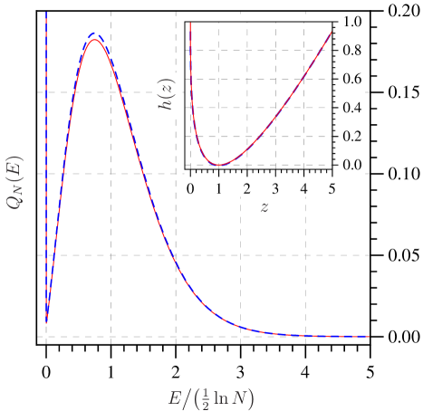
Figure 5: (Color online). Main: Distribution of the total energy for $N=2000$. The solid (red) line plots the saddle-point approximation Eq. (80), and the dashed (blue) line plots the exact form Eq. (69), evaluated using Mathematica. Inset: The solid (red) line plots the large deviation function Eq. (81), and the dashed (blue) line plots $-(\ln N)^{-1}\ln Q_{N}\bigl{(}\frac{z}{2}\ln N\bigr{)}-(\ln N)^{-1}\ln\bigl{[}(\frac{3\pi}{2}\ln N)^{1/2}z^{5/6}\,\Gamma(z^{1/3})\bigr{]}$ as a function of $z$, using the exact form of $Q_{N}(E)$ given in Eq. (69).

VI Summary and Conclusion

In summary, we have studied analytically various statistical properties in the final fan state of a one dimensional sticky gas of $N$ particles. The particles are initially distributed randomly in space, each with unit mass and with an initial velocity drawn independently from an identical distribution $\phi(v)$. Each particle moves ballistically and when two particles collide, they form a single cluster with the total mass and total momentum conserved in the collision process. In the long time limit, the system reaches a fan state where the system consists of a finite number of clusters with their velocities increasing from left to right and there is no further collision. We have shown that the sizes and the number of clusters are distributed universally in the fan state, independent of $\phi(v)$ and this distribution is identical to that of the cycles lengths in random permutation problem. We have also computed exactly the distribution of the size and the velocity of the rightmost cluster (leader) moving with the largest velocity. Furthermore, the distribution of the total energy in the fan state is also computed exactly for Gaussian $\phi(v)$. Our results provide an exactly solvable case of a many-body system (of finite size $N$) with dissipative dynamics and in particular, brings out the universal features of the final stationary state in an explicit way.

There are interesting open issues for further research. Here we have focused solely on the final fan state. It would be interesting to study the dynamics, i.e., the approach to this fan state and investigate to what extent the universal features exist away from the fan state.

There are also immediate generalizations of the problem studied here that are open for future research. For example, it would be interesting to know to what extent the universal features in the fan state remain valid for an inhomogeneous sticky gas. The inhomogeneity can arise either from unequal initial masses or nonidentical velocity distributions in the initial condition. For an infinite system, i.e., with a finite density of initial particles, the ballistic aggregation model with inhomogeneous initial condition has been studied FJM . It would be interesting to extend this study to the case of a finite number $N$ of particles.

Finally, it would be interesting to study this finite system of $N$ particles when the collisions are inelastic, but not necessarily sticky, i.e., with a nonzero coefficient of restitution. This problem has been studied for an infinite system and many asymptotic properties such as the energy decay and the velocity distribution were found to be similar to the sticky gas limit bennaim1 ; shinde . It would be interesting to see to what extent the universal features in the stationary state for finite $N$ are retained when one introduces a nonzero coefficient of restitution.

Acknowledgements: We thank D. Dhar for many stimulating discussions and for his early participation in this work. We acknowledge useful discussions with A. Comtet, P. L. Krapivsky and Y. Peres. The support from grant no. 3404-2 of “Indo-French Center for the Promotion of Advanced Research (IFCPAR/CEFIPRA)” is also gratefully acknowledged.

Appendix A Proof of Equation (15)

In this Appendix, we derive the distribution of the cluster sizes (regardless of their positions) starting from joint probability distribution of the cluster sizes and velocities given in Eq. (2). To calculate $\text{Pr}\{c_{1},c_{2},\dotsc,c_{N}\}$ from the joint-PDF $p_{N}(k;\{n_{i},u_{i}\})$, we must: (i) integrate out the velocities, (ii) sum over all configurations with the same cluster sizes (but placed in different orders) (iii) change the variables from the list $(n_{1},,\dotsc,n_{k})$ that represents the sizes of the $k$ consecutive clusters to the set $\{c_{1},\dotsc,c_{N}\}$ that encodes the number of clusters of a given size. We thus have

$$\text{Pr}\{c_{1},c_{2},\dotsc,c_{N}\}=\sum_{\begin{subarray}{c}\hbox{Permutations of}\\ \hbox{unequal size clusters}\end{subarray}}p_{N}(n_{1},\ldots,n_{k})\,,$$ (82)

where the sum is restricted to permutations that exchange clusters having different sizes i.e. permutations of the list $(n_{1},\ldots,n_{k})$ that exchange $n_{i}$’s having different values. Using Eq. (3) and the fact that $\prod_{i=1}^{k}n_{k}=\prod_{j=1}^{N}j^{c_{j}}$, we find that $p_{N}(n_{1},\ldots,n_{k})$ is given by

$$p_{N}(n_{1},\ldots,n_{k})=\frac{\delta\left(N-\sum_{j=1}^{N}jc_{j}\right)}{\prod_{j=1}^{N}j^{c_{j}}}\,\int\prod_{\ell=1}^{k}du_{\ell}\,{\mathcal{P}}(n_{\ell},u_{\ell})\prod_{\ell=1}^{k-1}\theta(u_{\ell+1}-u_{\ell})\,.$$ (83)

From the definition of ${\mathcal{P}}(n_{\ell},u_{\ell})$ given in Eq. (4), the integral on the r.h.s of Eq. (83) is found to be

$$\int\prod_{i=1}^{N}dv_{i}\,\phi(v_{i})\,\,\prod_{\ell=1}^{k-1}\theta\left(\frac{1}{n_{\ell+1}}{\sum_{j=N_{\ell}+1}^{N_{\ell+1}}v_{j}}-\frac{1}{n_{\ell}}{\sum_{j=N_{\ell-1}+1}^{N_{\ell}}v_{j}}\right)$$ (84)

where $N_{\ell}=n_{1}+\ldots+n_{\ell}$ for $\ell=1,\ldots,k$. The proof of Eq. (15) hence reduces to showing the following identity:

$$\sum_{\begin{subarray}{c}\hbox{Permutations of}\\ \hbox{unequal clusters}\end{subarray}}\int\prod_{i=1}^{N}dv_{i}\,\phi(v_{i})\,\,\prod_{\ell=1}^{k-1}\theta\left(\frac{1}{n_{\ell+1}}{\sum_{j=N_{\ell}+1}^{N_{\ell+1}}v_{j}}-\frac{1}{n_{\ell}}{\sum_{j=N_{\ell-1}+1}^{N_{\ell}}v_{j}}\right)=\frac{1}{c_{1}!\,c_{2}!\ldots c_{N}!}\,,$$ (85)

where we recall that $c_{1}$ is equal to the total number of 1’s in the list $(n_{1},\ldots,n_{k})$, $c_{2}$ is equal to the total number of 2’s in this list etc… This identity is proved by the following argument: consider a permutation that exchanges two clusters of the same size $p$; then, by relabeling the $v_{i}$ (which are dummy variables) we observe that the integral on the left hand side (l.h.s) of Eq. (85) is invariant. There are $c_{p}!$ possible permutations of the $c_{p}$ clusters of size $p$. Thus we have formally

$$c_{1}!\,c_{2}!\ldots c_{N}!\sum_{\begin{subarray}{c}\hbox{Permutations of}\\ \hbox{unequal clusters}\end{subarray}}=\sum_{\hbox{All Permutations}}\,.$$ (86)

If we have $k$ distinct numbers $u_{1}\ldots u_{k}$ there is only one permutation that orders them in increasing order. Therefore, we have

$$\sum_{\sigma\in\Sigma_{k}}\prod_{\ell=1}^{k-1}\theta(u_{\sigma(\ell+1)}-u_{\sigma(\ell)})=1\,,$$ (87)

where $\Sigma_{k}$ is the symmetric group of $k$ elements. After substituting this identity in Eq. (86) and using the fact that the PDF $\phi(v_{i})$ is normalized, Eq. (85) is finally proved. We note that the method of proof used here is closely related to the derivation by F. Spitzer of a generalization of the Sparre-Andersen theorem spitzer .

Appendix B Limiting Behavior of $F(z)$ as $z\to 0$ in Eq. (50)

Let us write $F(z)$ in Eq. (50) as $F(z)=\exp[-S(z)]$ where the sum

$$S(z)=\sum_{n=1}^{\infty}\frac{1}{2n}\,{\rm erfc}\left(\sqrt{\frac{n}{2}}\,z\right).$$ (88)

We want to compute the behavior of $S(z)$ as $z\to 0$. We first note the identity

$$\sum_{n=1}^{\infty}\frac{1}{2n}\,\exp(-n\,z^{2}/2)=-\frac{1}{2}\,\ln\left[1-e^{-z^{2}/2}\right].$$ (89)

Subtracting Eq. (89) from Eq. (88) gives

$$S(z)+\frac{1}{2}\,\ln\left[1-e^{-z^{2}/2}\right]=\sum_{n=1}^{\infty}\frac{1}{2n}\,\left[{\rm erfc}\left(\sqrt{\frac{n}{2}}\,z\right)-e^{-n\,z^{2}/2}\right].$$ (90)

Now, let us define a new variable $y=n\,z^{2}/2$. As $n$ changes by $1$, $y$ changes by $\Delta y=z^{2}/2$. Now, in the limit $z\to 0$, this increment $\Delta y$ is very small. Thus, one can replace the sum over $n$ on the r.h.s of Eq. (90) by an integral over $y$ to leading order for small $z$, giving

$$S(z)+\frac{1}{2}\,\ln\left[1-e^{-z^{2}/2}\right]\approx I=\frac{1}{2}\,\int_{0}^{\infty}\frac{dy}{y}\,\left[{\rm erfc}\left(\sqrt{y}\right)-e^{-y}\right].$$ (91)

The integral $I$ on the r.h.s is just a constant and can be evaluated by parts

$$I=-\frac{1}{2}\left[\int_{0}^{\infty}\,e^{-y}\,\ln(y)\,dy-\frac{1}{\sqrt{\pi}}\int_{0}^{\infty}\frac{\ln(y)}{\sqrt{y}}\,e^{-y}\,dy\right].$$ (92)

The two integrals on the r.h.s are elementary ones and can be easily evaluated to give finally, $I=-\ln(2)$. Substituting this in Eq. (90) and taking the $z\to 0$ limit gives

$$S(z)\to-\ln(\sqrt{2}\,z),$$ (93)

implying as $z\to 0$ to leading order

$$F(z)=\exp[-S(z)]\to\sqrt{2}\,z.$$ (94)

References

- (1) G. F. Carnevale, Y. Pomeau, and W. R. Young, Phys. Rev. Lett. 64, 2913 (1990).
- (2) Granular Gases, edited by T. Pöschel and S. Luding (Springer, Berlin, 2001); Granular Gas Dynamics, edited by T. Pöschel and N. Brilliantov (Springer, Berlin, 2003).
- (3) S. F. Shandarin and Ya. B. Zeldovich, Rev. Mod. Phys. 61, 185 (1989).
- (4) P. A. Martin, J. Piasecki, J. Stat. Phys, 76, 447 (1994); J. Stat. Phys, 84, 837 (1996).
- (5) J. M. Burgers, The Nonlinear Diffusion Equation (Reidel, Dordrecht,1974).
- (6) S. Kida, J. Fluid Mech. 93 part 2, 337 (1979).
- (7) U. Frisch and J. Bec, “Burgulence”, in Les Houches 2000: New Trends in Turbulence, M. Lesieur ed., (Springer EDP-Sciences).
- (8) L. Frachebourg, Phys. Rev. Lett. 82, 1502 (1999).
- (9) L. Frachebourg, P. A. Martin and J. Piasecki, Physica A 279, 69 (2000).
- (10) K. Shida and T. Kawai, Physica A 162, 145 (1989).
- (11) M. Sibuya, T. Kawai, and K. Shida, Physica A 167, 676 (1990).
- (12) H. Hyuga, T. Kawai, K. Shida and S. Yamada, Physica A 241, 664 (1997).
- (13) V. Goncharov, Sur la distribution des cycles dans les permutations, C.R. (Doklady) Acad. Sci. URSS (N.S) 35, 267 (1942).
- (14) L.A. Shepp, S.P. Lloyd, Trans. Am. Math. Soc. 121, 340 (1966).
- (15) F. Spitzer, Trans. Am. Math. Soc. 82, 323 (1956).
- (16) J. M. Steele, J. Comput. Appl. Math. 142, 235 (2002).
- (17) E. Trizac and P. L. Krapivsky, Phys. Rev. Lett. 91, 218302 (2003).
- (18) W. Feller, An Introduction to Probability Theory and Its Applications (Wiley, New York, 1971), Vol. II, 2nd ed.
- (19) R. L. Graham, D. E. Knuth and O. Patashnik, Concrete Mathematics (Addison-Wesley, 2nd ed., 1994).
- (20) J. Riordan, Introduction to Combinatorial Analysis (Dover, New York, 2002).
- (21) S. R. Finch, Mathematical Constants, (Cambridge University Press, UK, 2003).
- (22) R. Arratia, A. D. Barbour and S. Tavare, Notices of the AMS, 44, 903 (1997).
- (23) S.N. Majumdar and R.M. Ziff, Phys. Rev. Lett. 101, 050601 (2008).
- (24) C. Godreche and J.M. Luck, arXiv: 0809.3377.
- (25) P. Le Doussal and K.J. Wiese, arXiv: 0808.3217.
- (26) I. Bena and S.N. Majumdar, Phys. Rev. E 75, 051103 (2007); S. Sabhapandit, I. Bena, and S.N. Majumdar, JSTAT P05012 (2008).
- (27) R.A. Fisher and L.H.C. Tippet, Proc. Cambridge Philos. Soc. 24, 180 (1928); E.J. Gumbel, Statistics of Extremes (Columbia University Press, NY, 1958).
- (28) L. Frachebourg, V. Jacquemet, and P. A. Martin, J. Stat. Phys. 105, 745 (2001).
- (29) E. Ben-Naim, S.Y. Chen, G.D Doolen, and S. Redner, Phys. Rev. Lett. 83, 4069 (1999).
- (30) M. Shinde, D. Das, and R. Rajesh, Phys. Rev. Lett. 99, 234505 (2007).