Different thresholds of bond percolation in scale-free networks
with identical degree sequence

Abstract

Generally, the threshold of percolation in complex networks depends on the underlying structural characterization. However, what topological property plays a predominant role is still unknown, despite the speculation of some authors that degree distribution is a key ingredient. The purpose of this paper is to show that power-law degree distribution itself is not sufficient to characterize the threshold of bond percolation in scale-free networks. To achieve this goal, we first propose a family of scale-free networks with the same degree sequence and obtain by analytical or numerical means several topological features of the networks. Then, by making use of the renormalization group technique we determine the threshold of bond percolation in our networks. We find an existence of non-zero thresholds and demonstrate that these thresholds can be quite different, which implies that power-law degree distribution does not suffice to characterize the percolation threshold in scale-free networks.

I Introduction

As one of the best studied problems in statistical physics, percolation StAh92 is nowadays also the subject of intense research in the field of complex networks AlBa02 . In a network, if a fraction of its vertices (nodes, sites) or edges (links, bonds) is chosen independently with a probability $p$ to be “occupied”, it may undergo a percolation phase transition: when $p$ is above a threshold value $p_{c}$, called percolation threshold, the network possesses a giant component consisting of a finite fraction of interconnected nodes; otherwise, the giant component disappears and all nodes disintegrate into small clusters. So far, percolation in complex networks has received considerable attention in the community of statistical physics DoGoMe08 , because it is not only of high theoretical interest, but also relevant to many aspects of networks, including network security AlJeBa00 ; CoErAvHa00 ; CaNeStWa00 ; CoErAvHa01 , disease spread on networks MoNe00 ; Ne02 ; BoVePa03 ; Da05 ; ZhZhZoCh08 , etc.

Since global physical properties of random media alter substantially at the percolation threshold, which is central to understanding and applying this process, thus the precise knowledge of percolation threshold is extremely important ScZf08 . The issue of determining or calculating the percolation threshold has been the subject of intense study since the introduction of the model over half a century ago BrHa57 ; Fl41 . Despite decades of effort, there is still no general method for computing the percolation threshold of arbitrary graphs, and rigorous solution for percolation threshold is confined to some special cases ScZf08 ; Sc06 ; Zf06 ; Pi06 , such as the Barabási-Albert (BA) network BaAl99 , two dimensional lattice, and some other lattices. In most cases (e.g. lattices in three dimensions or above), the percolation threshold is estimated with numerical simulations, which are often time-consuming NeZi01 . Thus, finding the threshold exactly is essential to investigating the percolation problem on a particular graph Zf06 .

Perhaps the main reason for studying percolation in complex networks is to understand how the percolation properties are influenced by underlying topological structure. It has been established that degree distribution has a qualitative impact on the percolation. Recent studies indicated that in uncorrelated scale-free networks the percolation threshold is absent CoErAvHa00 ; CaNeStWa00 . Then a lot of other jobs followed, studying the influences of other properties on the percolation properties in scale-free networks; these include degree correlations BoVePa03 ; VaMo03 , clustering coefficient SeBo06 , and so forth. It was found that, degree correlations and clustering coefficient can strongly affect some percolation properties, but they cannot restore a finite percolation threshold in scale-free networks. This raises the question as to whether scale-free degree distribution is the only ingredient responsible for the absence of the percolation threshold. In other words, whether power-law degree distribution suffices to characterize the zero percolation threshold in scale-free networks.

In this paper, we study the effects of power-law degree distribution on the percolation threshold in scale-free networks. To this end, we first construct a class of scale-free networks with identical degree sequence by introducing a control parameter $q$. We then study analytically or numerically the topological features of the networks and show that this class of networks has unique topologies. Finally, using the renormalization-group theory, we investigate analytically the bond percolation problem in the considered networks, and find the existence of non-zero percolation thresholds depending on parameter $q$. Our findings indicate that the degree distribution by itself is not enough to characterize the percolation thresholds in scale-free networks. On the other hand, since our networks have the same degree sequence and thus the same degree distribution, the model proposed here can serve as a useful tool (substrate model) to check the impact of power-law degree distribution on the dynamical processes taking place on top of scale-free networks.

II Network construction and structural characteristics

In this section, we study the construction and structural properties of the networks under consideration, with focus on degree distribution, clustering coefficient, and average path length (APL).

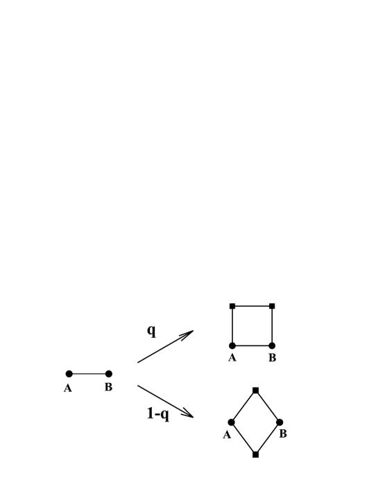
Figure 1: Iterative construction method of the networks. Each link is replaced by either of the connected clusters on the right-hand side of arrows with a certain probability, where black squares represent new vertices.

II.1 Construction algorithm

The proposed networks (graphs) are constructed in an iterative way as shown in Fig. 1. Let $H_{t}$ ($t\geq 0$) denote the networks after $t$ iterations. Then the networks are built in the following way: for $t=0$, the initial network $H_{0}$ is two nodes connected by an edge. For $t\geq 1$, $H_{t}$ is obtained from $H_{t-1}$. We replace each existing link in $H_{t-1}$ either by a connected cluster of links on the top right of Fig. 1 with probability $q$, or by the connected cluster on the bottom right with complementary probability $1-q$. The growing process is repeated $t$ times, with the graphs obtained in the limit $t\to\infty$. Figures 2 and 3 show the growth process of two networks for two limiting cases of $q=0$ and $q=1$, respectively.

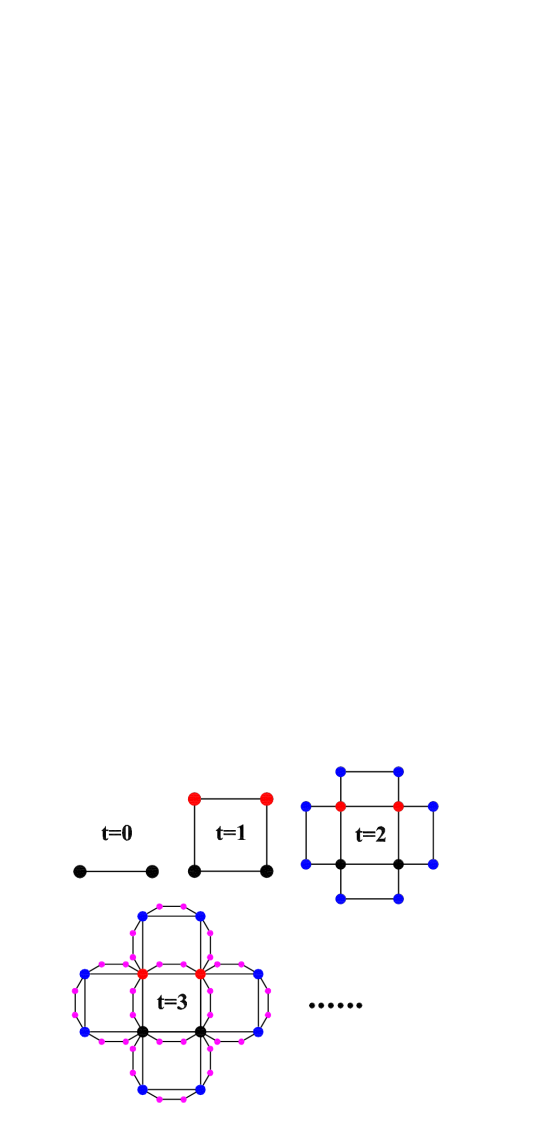
Figure 2: (Color online) Illustration of the first four evolution steps of the network growth process for the particular case $q=1$.

Figure 3: Sketch of the iteration process of the network for the particular case of $q=0$.

Now we compute some related quantities such as the number of total nodes and edges in $H_{t}$, called network order and size, respectively. Let $L_{v}(t)$ be the number of nodes generated at step $t$, and $E_{t}$ the total number of edges present at step $t$. Then $L_{v}(0)=2$ and $E_{0}=1$. By construction (see Fig. 1), we have $E_{t}=4E_{t-1}=4^{t}$ ($t\geq 0$). On the other hand, each existing edge at a given step will yield two new nodes at next step, this leads to $L_{v}(t)=2E_{t-1}=2\times 4^{t-1}$ ($t\geq 1$). Then the number of total nodes $N_{t}$ present at step $t$ is

$$N_{t}=\sum_{t_{i}=0}^{t}L_{v}(t_{i})=\frac{2}{3}(4^{t}+2).$$ (1)

The average node degree after $t$ iterations is $\langle k\rangle_{t}=\frac{2\,E_{t}}{N_{t}}=\frac{3\times 4^{t}}{4^{t}+2}$, which approaches 3 for large $t$.

II.2 Degree distribution

When a new node $i$ is added to the networks at a certain step $t_{i}$ ($t_{i}\geq 1$), it has a degree of 2. We denote by $k_{i}(t)$ the degree of node $i$ at time $t$. By construction, the degree $k_{i}(t)$ evolves with time as $k_{i}(t)=2\,k_{i}(t-1)=2^{t+1-t_{i}}$. That is to say, the degree of node $i$ increases by a factor 2 at each time step. Thus, the degree spectrum of the networks is discrete. In $H_{t}$ all possible degrees of nodes is 2, $2^{2}$ $2^{3}$, $\ldots$, $2^{t-1}$, $2^{t}$; and the number of nodes with degree $k=2^{t+1-m}$ is $n_{k}=L_{v}(m)=4^{m-1}$. Therefore, all class of networks $H_{t}$ have the same degree sequence (thus the same degree distribution) in the full range of $q$.

Since the degree spectrum of the networks is not continuous, it follows that the cumulative degree distribution Ne03 is given by $P_{\rm cum}(k)=\frac{N_{t,k}}{N_{t}}$, where $N_{t,k}=\sum_{k^{\prime}\geq k}n_{k^{\prime}}$ is the number of nodes whose degree is not less than $k$. When $t$ is large enough, we find $P_{\rm cum}(k)\sim k^{-2}$. So the degree distribution $P(k)$ of the networks follows a power-law form $P(k)\sim k^{-\gamma}$ with the exponent $\gamma=3$, independent of $q$. Notice that the same degree exponent has been obtained in the famous BA network BaAl99 .

II.3 Clustering Coefficient

By definition, the clustering coefficient WaSt98 of a node $i$ with degree $k_{i}$ is given by $C_{i}=2e_{i}/[k_{i}(k_{i}-1)]$, where $e_{i}$ is the number of existing triangles attached to node $i$, and $k_{i}(k_{i}-1)/2$ is the total number of possible triangles including $i$. The clustering coefficient of the whole network is the average over all individual $C_{i}^{\prime}s$. By construction, there are no triangles in $H_{t}$, so the clustering coefficient of every node and their average value in $H_{t}$ are both zero.

II.4 Average path length

Let $d_{ij}$ represent the shortest path length from node $i$ to $j$, then the average path length $d_{t}$ of $H_{t}$ is defined as the mean of $d_{ij}$ over all couples of nodes in the network:

$$d_{t}=\frac{D_{t}}{N_{t}(N_{t}-1)/2}\,,$$ (2)

where

$$D_{t}=\sum_{\begin{subarray}{c}i\in H_{t},\,j\in H_{t}\\ i\neq j\end{subarray}}d_{ij}$$ (3)

denotes the sum of the shortest path length between two nodes over all pairs.

For general $q$, it is difficult to derive a closed formula for the APL $d_{t}$ of $H_{t}$. But for two limiting cases of $q=1$ and $q=0$, both the networks are deterministic, we can obtain the analytic solutions for APL.

Figure 4: Second construction method of the network for $q=1$ case that highlights self-similarity: The graph after $t+1$ construction steps, $H_{t+1}$, is composed of four copies of $H_{t}$ denoted as $H_{t}^{\theta}$ $(\theta=1,2,3,4)$, which are connected to one another as above.

II.4.1 Case of $q=1$

In the special case (see Fig. 2), the networks are reduced to the $(1,3)$-flower proposed in RoHaAv07 . This limiting case of network has a self-similar structure that allows one to calculate $d_{t}$ analytically. The self-similar structure is obvious from an equivalent network construction method: to obtain $H_{t+1}$, one can make four copies of $H_{t}$ and join them in the hub nodes. As shown in Fig. 4, network $H_{t+1}$ may be obtained by the juxtaposition of four copies of $H_{t}$, which are consecutively labeled as $H_{t}^{1}$, $H_{t}^{2}$, $H_{t}^{3}$, and $H_{t}^{4}$. Then we can write the sum $D_{t+1}$ as

$$D_{t+1}=4\,D_{t}+\Delta_{t}\,,$$ (4)

where $\Delta_{t}$ is the sum of length over all shortest paths whose end points are not in the same $H_{t}$ branch.

The paths that contribute to $\Delta_{t}$ must all go through at least one of the four connecting nodes (i.e., $W$, $X$, $Y$ and $Z$ in Fig. 4) at which the different $H_{t}$ branches are connected. The analytical expression for $\Delta_{t}$, called the length of crossing paths, is found below.

Denote $\Delta_{t}^{\alpha,\beta}$ as the sum of length for all shortest paths with end points in $H_{t}^{\alpha}$ and $H_{t}^{\beta}$, respectively. If $H_{t}^{\alpha}$ and $H_{t}^{\beta}$ meet at a connecting node, $\Delta_{t}^{\alpha,\beta}$ rules out the paths where either end point is that shared connecting node. For example, each path contributed to $\Delta_{t}^{1,2}$ should not end at node $W$. If $H_{t}^{\alpha}$ and $H_{t}^{\beta}$ do not meet, $\Delta_{t}^{\alpha,\beta}$ excludes the paths where either end point is any connecting node. For instance, each path contributed to $\Delta_{t}^{1,3}$ should not end at nodes $W$, $X$, $Y$ or $Z$. Then the total sum $\Delta_{t}$ is

$$\Delta_{t}= \,\Delta_{t}^{1,2}+\Delta_{t}^{1,3}+\Delta_{t}^{1,4}+\Delta_{t}^{2,3}+\Delta_{t}^{2,4}+\Delta_{t}^{3,4}-4.$$ (5)

The last term at the end compensates for the overcounting of certain paths: the shortest path between $W$ and $Y$, with length $2$, is included in $\Delta_{t}^{1,4}$ and $\Delta_{t}^{2,3}$; the shortest path between $X$ and $Z$, also with length $2$, is included in both $\Delta_{t}^{1,2}$ and $\Delta_{t}^{3,4}$.

By symmetry, $\Delta_{t}^{1,2}=\Delta_{t}^{1,4}=\Delta_{t}^{2,3}=\Delta_{t}^{3,4}$ and $\Delta_{t}^{1,3}=\Delta_{t}^{2,4}$, so that

$$\Delta_{t}=4\Delta_{t}^{1,2}+2\Delta_{t}^{1,3}-4.$$ (6)

In order to find $\Delta_{t}^{1,2}$ and $\Delta_{t}^{1,3}$, we define quantity $s_{t}$ as

$$s_{t}=\sum_{\begin{subarray}{c}i\in H_{t}\\ i\neq W\end{subarray}}d_{iW}\,.$$ (7)

Considering the self-similar network structure, we can easily know that at time $t+1$, the quantity $s_{t+1}$ evolves recursively as

$$s_{t+1} = 2\,s_{t}+\left[s_{t}+(N_{t}-1)\right]+\left[s_{t}+(N_{t}-1)-2\right]$$ (8)

$$= 4\,s_{t}+\frac{4}{3}(4^{t}-1).$$

Using $s_{1}=4$, we have

$$s_{t}=\frac{1}{9}\left(4+5\times 4^{t}+3\,t\times 4^{t}\right).$$ (9)

On the other hand, by definition given above, we have

$$\Delta_{t}^{1,2} = \sum_{\begin{subarray}{c}i\in H_{t}^{1},\,\,j\in H_{t}^{2}\\ i,j\neq W\end{subarray}}d_{ij}$$ (10)

$$= \sum_{\begin{subarray}{c}i\in H_{t}^{1},\,\,j\in H_{t}^{2}\\ i,j\neq W\end{subarray}}(d_{iW}+d_{jW})$$

$$= (N_{t}-1)\sum_{\begin{subarray}{c}i\in H_{t}^{1}\\ i\neq W\end{subarray}}d_{iW}+(N_{t}-1)\sum_{\begin{subarray}{c}j\in H_{t}^{2}\\ j\neq W\end{subarray}}d_{jW}$$

$$= 2(N_{t}-1)\sum_{\begin{subarray}{c}i\in H_{t}^{1}\\ i\neq W\end{subarray}}d_{iW}$$

$$= 2(N_{t}-1)\,s_{t}.$$

Continue analogously,

$$\Delta_{t}^{1,3} = \sum_{\begin{subarray}{c}i\in H_{t}^{1},\,i\neq W,Z\\ j\in H_{t}^{3},j\neq X,Y\end{subarray}}d_{ij}$$ (11)

$$= \sum_{\begin{subarray}{c}i\in H_{t}^{1},\,i\neq W,Z\\ d_{iW}<d_{iZ}\\ j\in H_{t}^{3},j\neq X,Y\end{subarray}}(d_{iW}+d_{WX}+d_{jX})$$

$$+\sum_{\begin{subarray}{c}i\in H_{t}^{1},\,i\neq W,Z\\ d_{iZ}<d_{iW}\\ j\in H_{t}^{3},j\neq X,Y\end{subarray}}(d_{iZ}+d_{ZY}+d_{jY})$$

$$= 2\,\sum_{\begin{subarray}{c}i\in H_{t}^{1},\,i\neq W,Z\\ d_{iW}<d_{iZ}\\ j\in H_{t}^{3},j\neq X,Y\end{subarray}}(d_{iW}+d_{WX}+d_{jX})\,,$$

where the symmetry property has been used. After simple calculations, we obtain

$$\Delta_{t}^{1,3}=2(N_{t}-1)\,s_{t} + (N_{t}-1)^{2}-2\left(\frac{N_{t}}{2}\right)^{2}$$ (12)

$$- 2(s_{t}+N_{t}-3)-1.$$

Substituting Eqs. (10) and (12) into Eq. (6), we obtain after simplification

$$\Delta_{t}=\frac{4}{9}\left(-2+11\times 16^{t}+6\,t\times 16^{t}\right).$$ (13)

Thus

$$D_{t+1}=4\,D_{t}+\frac{4}{9}\left(-2+11\times 16^{t}+6\,t\times 16^{t}\right).$$ (14)

Using $D_{1}=8$, Eq. (14) is solved inductively,

$$D_{t}=\frac{1}{27}\left(8+16\times 4^{t}+3\times 16^{t}+6t\times 16^{t}\right).$$ (15)

Inserting Eq. (15) into Eq. (2), one can obtain the analytical expression for $d_{t}$:

$$d_{t}=\frac{2}{3}\times\frac{8+16\times 4^{t}+3\times 16^{t}+6t\times 16^{t}}{4\times 16^{t}+10\times 4^{t}+4},$$ (16)

which approximates $t$ in the infinite $t$, implying that the APL shows a logarithmic scaling with network order. Therefore, in the case of $q=1$, the network exhibits a small-world behavior. We have checked our analytic result against numerical calculations for different network order up to $t=10$ which corresponds to $N_{10}=1048577$. In all the cases we obtain a complete agreement between our theoretical formula and the results of numerical investigation.

II.4.2 Case of $q=0$

For this particular case, our networks turn out to be the hierarchical lattice introduced in BeOs79 , which is also self-similar. Using a method similar to but a little different from that applied in preceding subsection, we can compute analytically the average path length $d_{t}$. We omit the calculation process and give only the exact expression as below:

$$d_{t}=\frac{22\times 2^{t}\times 16^{t}+8^{t}(21t+42)+27\times 4^{t}+98\times 2^{t}}{42\times 16^{t}+105\times 4^{t}+42}.$$ (17)

Equation (17) recovers the previously obtained result in HiBe06 and has been confirmed by extensive numerical simulations. In the large $t$ limit, $d_{t}\sim\frac{11}{21}2^{t}$. On the other hand, for large $t$ limit, $N_{t}\sim 4^{t}$, so $d_{t}$ grows as a square root of the number of network nodes. Thus, in the case of $q=0$, the network exhibits a ‘large-world’ behavior of typical node-node distances.

II.4.3 Case of $0<q<1$

For $0<q<1$, in order to obtain the variation of the average path length with the parameter $q$, we have performed extensive numerical simulations for different $q$ between 0 and 1. Simulations were performed for network $N_{7}$ with order $10924$, averaging over 20 network samples for each value of $q$. In Fig. 5, we plot the average path length as a function of $q$. We observe that, when $q$ increases from 0 to 1, the average path length drops drastically from a very high value to a small one, which shows that there is a crossover between small-world and ‘large-world’. This behavior is similar to that in the WS model WaSt98 .

Figure 5: Graph of the dependence of the average path length on the tunable parameter $q$.

III Threshold of bond percolation

As discussed in previous section, the networks exhibit many interesting properties, i.e., they have the same degree sequence independent of parameter $q$; they are scale-free and non-clustered; and they display a crossover between “large-world” and small-world. All these features are not shared simultaneously by any previously reported networks. Hence, it is worthwhile to investigate the processes taking place upon the model to find the different impact on dynamic precesses compared with other networks such as the BA network. In what follows we will study bond percolation, which is one of the most important issues in statistical physics StAh92 .

In bond percolation every bond (link or edge) on a specified graph is independently either “occupied” with probability $\lambda$, or not with the complementary probability $1-\lambda$. In our case the percolation problem can be solved using the real-space renormalization group technique Mi75 ; Mi76 ; Ka76 ; Do03 ; RoAv07 , giving exact solution for the interesting quantity of percolation threshold. Let us describe the procedure in application to the network considered. Assuming that the network growth stops at a time step $t\rightarrow\infty$, when the network is spoiled in the following way: for a link present in the undamaged network, with the probability $\lambda$ we retain it in the damaged network. Then we invert the transformation in Fig. 1 and define $n=t-\tau$ for this inverted transformation, which is actually a decimation procedure Do03 . Further, we introduce the probability $\lambda_{n}$ that if two nodes are connected in the undamaged network at $\tau=t-n$, then at the $n$th step of the decimation for the damaged network, there exists a path between these vertices. Here, $\lambda_{0}=\lambda$. We can easily obtain the following recursion relation for $\lambda_{n}$

$$\lambda_{n+1}=q\,(\lambda_{n}+\lambda_{n}^{3}-\lambda_{n}^{4})+(1-q)(2\lambda_{n}^{2}-\lambda_{n}^{4}).$$ (18)

Equation (18) has four roots (i.e., fixed points), among which the root $\lambda=-\frac{1-q}{2}-\frac{1}{2}\sqrt{5-6q+q^{2}}$ is invalid, because it is less than 0. The other three fixed points are as follows: two stable fixed points at $\lambda=0$ and $\lambda=1$, and an unstable fixed point at $\lambda_{c}$ that is the percolation threshold. The reason for the unstable fixed point corresponding to the threshold is as follows: at any $0<\lambda_{0}<\lambda_{c}$, $\lambda_{n}$ approaches 0 as $n\rightarrow\infty$, which means there is no percolation; while at any $\lambda_{c}<\lambda_{0}<1$, $\lambda_{n}$ approach 1, indicating an existence of the percolating cluster.

The exact expression of $\lambda_{c}$ as a function of $q$ is

$$\lambda_{c}=-\frac{1-q}{2}+\frac{1}{2}\sqrt{5-6q+q^{2}}.$$ (19)

Interestingly, for the case of $q=0$, $\lambda_{c}$ is equal to $\frac{\sqrt{5}-1}{2}$, which is the inverse of the golden ratio $\phi$ ($\phi=\frac{\sqrt{5}+1}{2}$) and is the same value as the site percolation threshold for the “B” lattice discussed in Sc06 ; Zf06 . We present the dependence of $\lambda_{c}$ on $q$ in Fig. 6, which indicates that the threshold $\lambda_{c}$ decreases as $q$ increases. When $q$ grows from 0 to 1, $\lambda_{c}$ decreases from $\frac{\sqrt{5}-1}{2}\approx 0.618$ to 0.

Figure 6: The dependence relation of percolation threshold $\lambda_{c}$ on the parameter $q$.

Thus, in a large range of parameter $q$ (i.e., $q<1$), there exists a critical non-zero percolation threshold $\lambda_{c}$ such that for $\lambda>\lambda_{c}$ a giant component appears spanning the entire network, for $\lambda<\lambda_{c}$ there are only isolated small clusters. The existence of percolation thresholds in our networks is in sharp contrast with the null threshold found in a wide range of previously studied scale-free networks CoErAvHa00 ; CaNeStWa00 ; BoVePa03 ; VaMo03 ; SeBo06 .

Note that since the susceptible-infected-removed (SIR) model can be mapped to the bond percolation problem MoNe00 ; Ne02 ; BoVePa03 , for the SIR model on our networks the epidemic prevalence undergoes a phase transition at a finite threshold $\lambda_{c}$ of the transmission probability. If infection rate is above $\lambda_{c}$, the disease spreads and infects a finite fraction of the population. On the contrary, when infection rate is below $\lambda_{c}$, the total number of infected individuals is infinitesimally small in the limit of very large populations. The existence of epidemic thresholds in the present networks is compared to the result for some other scale-free networks, where arbitrarily small infection rate shows finite prevalence MoPaVe02 .

From Eq. (19), one can see that for different $q$, the networks have distinct percolation thresholds. As known from preceding section, the whole class of the networks exhibits identical degree sequence (power-law degree distribution) and (zero) clustering coefficient, which shows that degree distribution and clustering coefficient are not sufficient to characterize the threshold of bond percolation in scale-free networks. One may ask why the considered networks have disparate percolation thresholds. We speculate that the diverse thresholds in our networks lie with the average path length, which needs further confirmation in the future.

IV Conclusions

We have demonstrated that power-law degree distribution alone does not suffice to characterize the percolation threshold on scale-free networks under bond percolation. To this end, by introducing a parameter $q$, we have presented a family of scale-free networks with the same degree sequence and (zero) clustering coefficient. We provided a detailed analysis of the topological features and showed that the model exhibits a rich structural behavior. In particular, using a renormalization method, we have derived an exact analytic expression for the thresholds of bond percolation in our networks. We found that finite thresholds are recovered for our networks in the case of $q<1$, which is in contrast to the conventional wisdom that null percolation threshold is an intrinsic nature of scale-free networks. Therefore, care should be needed when making general statements about the percolation problem in scale-free networks.

It should be mentioned that the model generation of scale-free networks with the same degree sequence is a very common problem in complex network research. Actually, in the study of the impacts of other characteristics (besides degree distribution) of scale-free networks on the dynamical processes defined on the networks, the interference of power-law degree distribution should be avoided. In this case, such a model is necessitated. Traditionally, the interchanging algorithm (through rewiring two links between four end points) is frequently used to achieve this goal MaSn02 . But this algorithm may lead to disconnection of the whole network. We have shown that the scale-free networks proposed here have identical degree sequence and are always connected. So our networks can overcome above deficiency. They may be helpful for investigating how other features (say, average path length), other than power-law degree distribution, are relevant to the performance of scale-free networks.

Finally, we stress that since we were only concerned with the percolation phase transition point, we merely gave the exact position of the percolation thresholds, omitting some other properties of bond percolation, such as the value of the critical exponents governing behavior close to the transition, the complete distribution of the cluster sizes, and closed-form expressions for the mean and variance of the distribution. All these are worth studying further in the future, which is beyond the scope of this paper.

Note added.—A relevant publication WaSaSo02 about bond percolation has come to our attention, where the authors showed that different percolation thresholds exist for different networks having the same degree distribution (not degree sequence as addressed in this present paper).

- (1) D. Stauffer and A. Aharony, Introduction to Percolation Theory, 2nd ed. (Taylor and Francis, London, 1992).
- (2) R. Albert and A.-L. Barabási, Rev. Mod. Phys. 74, 47 (2002).
- (3) S. N. Dorogovtsev, A. V. Goltsev and J. F. F. Mendes, Rev. Mod. Phys. 80, 1276 (2008).
- (4) R. Albert, H. Jeong, A.-L. Barabási, Nature (London) 406, 378 (2000).
- (5) D. S. Callaway, M. E. J. Newman, S. H. Strogatz, and D. J. Watts, Phys. Rev. Lett. 85, 5468 (2000).
- (6) R. Cohen, K. Erez, D. ben-Avraham, S. Havlin, Phys. Rev. Lett. 85, 4626 (2000).
- (7) R. Cohen, K. Erez, D. ben-Avraham, S. Havlin, Phys. Rev. Lett. 86, 3682 (2001);
- (8) C. Moore and M. E. J. Newman, Phys. Rev. E 61, 5678 (2000).
- (9) M. E. J. Newman, Phys. Rev. E 66, 016128 (2002).
- (10) M. Boguñá, R. Pastor-Satorras and A. Vespignani, Phys. Rev. Lett. 90, 028701 (2003).
- (11) L. Dall’Asta, J. Stat. Mech.: Theory Exp. P08011 (2005).
- (12) Z. Z. Zhang, S. G. Zhou, T. Zou, and G. S. Chen, J. Stat. Mech.: Theory Exp. P09008 (2008).
- (13) C. R. Scullard and R. M. Ziff, Phys. Rev. Lett. 100, 185701 (2008).
- (14) S. R. Broadbent and J. M. Hammersley, Proc. Cambridge Philos. Soc. 53, 629 (1957).
- (15) P. J. Flory, J. Am. Chem. Soc. 63, 3083 (1941).
- (16) C. R. Scullard, Phys. Rev. E 73, 016107 (2006).
- (17) R. M. Ziff, Phys. Rev. E 73, 016134 (2006).
- (18) W. Pietsch, Phys. Rev. E 73, 066112 (2006).
- (19) A.-L. Barabási and R. Albert, Science 286, 509 (1999).
- (20) M. E. J. Newman and R. M. Ziff, Phys. Rev. E 64, 016706 (2001).
- (21) A. Vázquez and Y. Moreno, Phys. Rev. E 67, 015101(R) (2003).
- (22) M. Á. Serrano and M. Boguñá, Phys. Rev. Lett. 97, 088701 (2006).
- (23) M. E. J. Newman, SIAM Rev. 45, 167 (2003).
- (24) D. J. Watts and H. Strogatz, Nature (London) 393, 440 (1998).
- (25) H. D. Rozenfeld, S. Havlin, and D. ben-Avraham, New J. Phys. 9, 175 (2007).
- (26) A. N. Berker and S. Ostlund, J. Phys. C 12, 4961 (1979).
- (27) M. Hinczewski and A. N. Berker, Phys. Rev. E 73, 066126 (2006).
- (28) A. A. Migdal, Zh. Eksp. Teor. Fiz. 69, 1457 (1975).
- (29) A. A. Migdal, Sov. Phys. JETP 42, 743 (1976).
- (30) L. P. Kadanoff, Ann. Phys. (N.Y.) 100, 359 (1976).
- (31) S. N. Dorogovtsev, Phys. Rev. E 67, 045102(R) (2003).
- (32) H. D. Rozenfeld and D. ben-Avraham, Phys. Rev. E 75, 061102 (2007).
- (33) Y. Moreno, R. Pastor-Satorrasand, and A. Vespignani, Eur. Phys. J. B 26, 521 (2002).
- (34) S. Maslov, K. Sneppen, Science 296, 910 (2002).
- (35) C. P. Warren, L. M. Sander, and I. M. Sokolov, Phys. Rev. E 66, 056105 (2002).