On the solar nickel and oxygen abundances

Abstract

Determinations of the solar oxygen content relying on the neutral forbidden transition at 630 nm depend upon the nickel abundance, due to a Ni i blend. Here we rederive the solar nickel abundance, using the same ab initio 3D hydrodynamic model of the solar photosphere employed in the recent revision of the abundances of C, N, O and other elements. Using 17 weak, unblended lines of Ni i together with the most accurate atomic and observational data available we find $\log\epsilon_{\rm Ni}=6.17\pm 0.02\,\mathrm{(statistical)}\pm 0.05\,\mathrm{(systematic)}$, a downwards shift of 0.06–0.08 dex relative to previous 1D-based abundances. We investigate the implications of the new nickel abundance for studies of the solar oxygen abundance based on the [O i] 630 nm line in the quiet Sun. Furthermore, we demonstrate that the oxygen abundance implied by the recent sunspot spectropolarimetric study of Centeno & Socas-Navarro needs to be revised downwards from $\log\epsilon_{\rm O}=8.86\pm 0.07$ to $8.71\pm 0.10$. This revision is based on the new nickel abundance, application of the best available $gf$-value for the 630 nm forbidden oxygen line, and a more transparent treatment of CO formation. Determinations of the solar oxygen content relying on forbidden lines now appear to converge around $\log\epsilon_{\rm O}=8.7$.

Table 1List of neutral nickel lines

Atomic levels				Isotope	Wavelength	Ex. Pot.	$\log gf$	$gf$	$\log\gamma_{\rm rad}$	$\sigma$	$\alpha$	Wλ	$\log\epsilon_{\rm Ni}$	Weight
Lower		Upper			(nm, air)	(eV)	(eff.)	ref.				(pm)	(3D)
3d8(3F)4s4p(3P)	5G4	3d9(2D)4d	3G5		474.01658	3.480	-1.730	WL	7.899	844	0.281	1.60	6.18	1
3d9(2D)4p	3P1	3d9(2D)4d	3P0	58Ni	481.19772		-1.592
				60Ni	481.19926	3.658	-2.006	J03	8.285	-	-	2.12	6.20	1
3d8(3F)4s4p(3P)	5G2	3d84s(4F)5s	5F3		481.45979	3.597	-1.620	WL	8.053	743	0.236	1.58	6.17	1
3d8(3F)4s4p(3P)	5G3	3d84s(4F)5s	5F4		487.47929	3.543	-1.450	WL	8.039	-	-	2.35	6.15	1
3d9(2D)4p	3D2	3d84s(4F)5s	5F2		488.67108	3.706	-1.780	WL	8.211	-	-	0.90	6.13	1
3d8(3F)4s4p(3P)	5G4	3d84s(4F)5s	5F5		490.09708	3.480	-1.670	WL	8.062	693	0.238	1.79	6.17	1
3d8(3F)4s4p(3P)	5F4	3d9(2D)4d	3G4		497.61348	3.606	-1.250	WL	7.962	843	0.282	2.86	6.13	2
3d8(3F)4s4p(3P)	5F4	3d84s(4F)5s	5F5		515.79805	3.606	-1.510	WL	8.093	691	0.236	1.86	6.13	3
3d8(3F)4s4p(3P)	3G5	3d84s(4F)5s	5F4		550.40945	3.834	-1.700	WL	8.063	713	0.240	0.97	6.18	1
3d9(2D)4p	1F3	3d9(2D)4d	3G4		551.00092	3.847	-0.900	WL	8.215	-	-	3.76	6.17	2
3d9(2D)4p	1F3	3d84s(4F)5s	5F4		553.71054	3.847	-2.200	WL	8.280	695	0.216	0.31	6.16	3
3d8(3F)4s4p(3P)	3G3	3d9(2D)4d	3G4	60Ni	574.92795		-2.526
				58Ni	574.93039	3.941	-2.112	WL	7.944	832	0.284	0.44	6.17	2
3d8(3F)4s4p(3P)	3F4	3d9(2D)4d	3G5	60Ni	617.67980		-0.816
				58Ni	617.68200	4.088	-0.402	WL	8.162	826	0.284	6.54	6.17	2
3d8(3F)4s4p(3P)	3F4	3d84s(4F)5s	5F4		620.46048	4.088	-1.100	WL	8.244	719	0.247	2.11	6.19	3
3d8(3F)4s4p(3P)	3F3	3d9(2D)4d	3G4	60Ni	622.39710		-1.466
				58Ni	622.39914	4.105	-1.052	WL	8.322	827	0.283	2.79	6.17	3
3d8(3F)4s4p(3P)	3D3	3d9(2D)4d	3G4	60Ni	637.82328		-1.386
				58Ni	637.82580	4.154	-0.972	WL	8.317	825	0.283	3.20	6.20	3
3d8(3F)4s4p(3P)	3D3	3d84s(4F)5s	5F4		641.45884	4.154	-1.180	WL	8.369	721	0.249	1.68	6.20	2

Note. — Wavelengths and excitation potentials are from Litzen et al. (1993). Radiative damping is from VALD (Kupka et al., 1999). Transition designations are from Wickliffe & Lawler (1997) except in the case of 481.2 nm, for which the designation is from VALD. References for $gf$-values are WL: Wickliffe & Lawler (1997) and J03: Johansson et al. (2003). For lines with isotopic components $gf$-values are effective only, rescaled to reflect the (terrestrial) isotopic fractions of Rosman & Taylor (1998). Collisional damping parameters $\alpha$ and $\sigma$ are courtesy of Paul Barklem (private communication, 1999; now in VALD, Barklem et al. 2000). Equivalent widths are from profile fits using the 3D model.

1. Introduction

The reference solar oxygen abundance has been revised over the past decade from $\log\epsilon_{\rm O}=8.93\pm 0.04$ (Anders & Grevesse, 1989) via $8.83\pm 0.06$ (Grevesse & Sauval, 1998, GS98) to $8.66\pm 0.05$ (Asplund et al., 2005, AGS05). This downward slide has been brought on by the tandem influences of three-dimensional photospheric models, treatment of departures from local thermodynamic equilibrium (LTE), identification of blends, improved atomic data and better observations (Allende Prieto et al., 2001; Asplund et al., 2004). The new abundances of oxygen and other elements have solved many outstanding problems, but ruined agreement between helioseismological theory and observation (see e.g. Basu & Antia, 2008). This has prompted a reanalysis of photospheric models, resulting in support for high (Ayres et al., 2006; Centeno & Socas-Navarro, 2008; Ayres, 2008), low (Scott et al., 2006; Socas-Navarro & Norton, 2007; Koesterke et al., 2008; Meléndez & Asplund, 2008) and intermediate (Caffau et al., 2008) solar oxygen abundances.

Many of these analyses rely upon the forbidden oxygen line at 630.0304 nm, known to contain a significant blend from Ni i at 630.0341 nm (Allende Prieto et al., 2001; Johansson et al., 2003). The strength of this blend, and therefore the $\epsilon_{\rm O}$ indicated by [O i] 630 nm, depend critically upon the solar nickel abundance ($\epsilon_{\rm Ni}$). This is no less true of the ingenious spectropolarimetric work of Centeno & Socas-Navarro (2008) than of any other study based on [O i] 630 nm. Here we accurately redetermine $\epsilon_{\rm Ni}$, and discuss the impact of the new value upon abundances from [O i] 630 nm. We show that $\epsilon_{\rm Ni}$ is model-dependent, contradicting claims by Centeno & Socas-Navarro that their technique allows a nearly model-independent analysis of $\epsilon_{\rm O}$.

2. Model atmospheres and observational data

We used the same 3D LTE model atmosphere and line formation code as in earlier papers (e.g. Asplund et al., 2000b, 2004), described by Asplund et al. (2000a). We performed comparative calculations with three 1D models: HM (Holweger & Müller, 1974), marcs (Gustafsson et al., 1975; Asplund et al., 1997) and 1DAV (a contraction of the 3D model into one dimension by averaging over surfaces of equal optical depth). Each 1D model included a microturbulent velocity $\xi_{\rm t}=1\,\mathrm{km\,s}^{-1}$. We averaged simulated intensity profiles over the temporal and spatial extent of the model atmosphere, and compared results with the Fourier Transform Spectrograph (FTS) disk-center atlas of Brault & Neckel (1987, see also ). We removed the solar gravitational redshift of 633 m s^-1, and convolved simulated profiles with an instrumental sinc function of width $\Delta\sigma=\frac{c}{R}=0.857$ km s^-1, reflecting the FTS resolving power $R=350\,000$ (Neckel, 1999). We obtained abundances with the 3D model from profile-fitting via a $\chi^{2}$-analysis, fitting local continua independently with nearby clear sections of the spectrum. For 1D models we used the equivalent widths of 3D profile fits.

3. Atomic data and line selection

Our adopted Ni i lines and atomic data are given in Table 1. The paucity of good lines and atomic data in the optical precludes any meaningful analysis of Ni ii in the Sun. The most accurate Ni i oscillator strengths come from the laboratory FTS branching fractions (BFs) of Wickliffe & Lawler (1997), put on an absolute scale with the time-resolved laser-induced fluorescence (TRLIF) lifetimes of Bergeson & Lawler (1993). A small number of high-quality $gf$-values are also available from Johansson et al. (2003), based upon FTS BFs and a single TRLIF lifetime. The uncertainties of the individual oscillator strengths we employ range from 0.02–0.07 dex, but most are accurate to $\pm 0.03$ dex.

Nickel has five stable isotopes: ⁵⁸Ni, ⁶⁰Ni, ⁶¹Ni, ⁶²Ni and ⁶⁴Ni, present in the approximate ratio 74:28:1:4:1 in the Earth (Rosman & Taylor, 1998). Isotopic splitting of optical lines is small, and dominated by ⁵⁸Ni and ⁶⁰Ni. Litzen et al. (1993) have obtained accurate laboratory FTS wavelengths for the isotopic components of many Ni i lines, which we include in Table 1 where applicable. We model such lines with two components, distributing the total oscillator strength according to the terrestrial ⁵⁸Ni:⁶⁰Ni ratio. We are confident that the available data sufficiently describe the isotopic broadening of solar lines, as laboratory FTS recordings are far better resolved than lines in the Sun. Isotopic structure has not been included in other determinations of the solar nickel abundance.

We gave weightings to lines from 1 to 3 according to the absence of blends in the solar spectrum and the clarity of the surrounding continuum. Along with 16 unblended weak lines, we include the somewhat stronger Ni i 617.7 nm (W${}_{\lambda}=6.54$ pm) owing to its clean line profile and its accurate atomic data. This line should be less affected by the rigors of strong line formation than single-component lines of the same equivalent width, thanks to the desaturating effects of isotopic broadening. To be conservative, we give this line a weighting of 2. Our list has only two lines in common with Biémont et al. (1980), mainly due to the absence of accurate $gf$-values for the 10 other lines used by those authors.

We took wavelengths and excitation potentials from Litzen et al. (1993), and radiative damping from VALD (Kupka et al., 1999). For most lines, we used collisional broadening parameters calculated for individual lines by Paul Barklem (private communication, 1999; now in VALD, Barklem et al. 2000). For the remainder we interpolated in the tables of Anstee & O’Mara (1995) and Barklem & O’Mara (1997) where possible. For Ni i 488.7 nm we used the traditional Unsöld (1955) formula with a scaling factor of 2.0. Transition designations are from Wickliffe & Lawler (1997), except for Ni i 481.2 nm, where the designation is from VALD. Apart from the slightly stronger 617.7 nm line, all our lines are quite insensitive to the adopted collisional broadening. The broadening treatment of Ni i 488.7 nm thus has no impact on our abundance determination, nor does the ambiguity in the identification of the upper level of Ni i 481.2 nm (Johansson et al., 2003).

Table 2Logarithmic solar nickel abundances (mean $\pm$ 1 standard deviation)

	3D	1DAV	HM	marcs	Meteoritic
$\log\epsilon_{\mathrm{Ni}}$ (Ni i lines)	$6.17\pm 0.02$	$6.17\pm 0.02$	$6.26\pm 0.02$	$6.16\pm 0.02$	$6.19\pm 0.03$

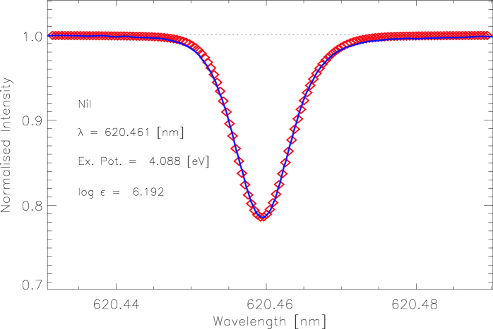
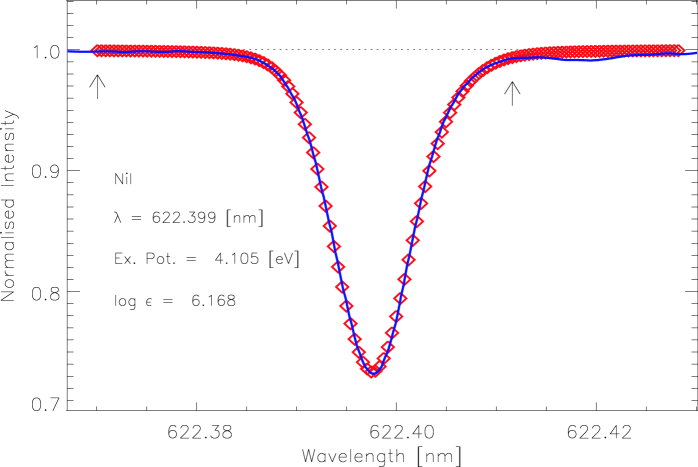
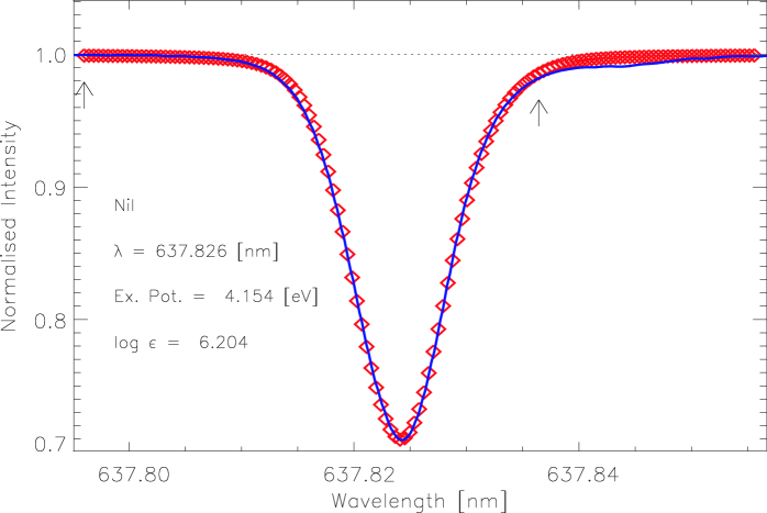
Figure 1.— Example spatially- and temporally-averaged, disk-center synthesized Ni i line profiles (diamonds), compared with observed FTS profiles (solid lines). We removed the solar gravitational redshift from the FTS spectrum, convolved synthesized profiles with instrumental sinc functions and fitted them in abundance and line shift. Arrows indicate the windows used for profile fits; in the uppermost panel, we used the entire synthesized region.

Figure 2.— Solar nickel abundances indicated by Ni i lines, as computed with different model atmospheres. No substantial trends with line strength are visible with any of the four models. The similarity between 3D and 1DAV abundances suggests that the mean temperature structure of the 3D model is predominantly responsible for the difference between HM and 3D results, rather than the presence of temperature inhomogeneities.

4. Nickel results

The mean nickel abundances we found using different model atmospheres are given in Table 2. Examples of profile fits to Ni i lines with the 3D model are given in Fig. 1, exhibiting similarly impressive agreement with observation as seen with other species (e.g. Asplund et al., 2000a, 2004). None of the models show abundance trends with equivalent width (Fig. 2), excitation potential nor wavelength, and the scatter is universally low, boding well for the internal consistency of all models. Very little difference exists between 3D and 1DAV abundances, implying that the mean temperature structure rather than atmospheric inhomogeneities is the main reason for the difference between the 3D and HM results. The 3D $\epsilon_{\rm Ni}$ is in excellent agreement with the meteoritic value (AGS05), whereas the HM value is not.

We adopt the 3D Ni i result as the best estimate of the solar abundance:

$$\epsilon_{\rm Ni}=6.17\pm 0.05.$$

The total error ($\pm$0.05 dex) is the sum in quadrature of the line-to-line scatter ($\pm$0.02 dex) and potential systematics arising from the model atmosphere ($\pm$0.05 dex). AGS05 gave $\epsilon_{\mathrm{Ni}}=6.23\pm 0.04$, from Reddy et al. (2003) using an atlas9 model (Kurucz, http://kurucz.harvard.edu/grids.html). Previous reviews (e.g. GS98, ) adopted $6.25\pm 0.09$, by Biémont et al. (1980) using the HM model. Our value is 0.06–0.08 dex lower than earlier ones, and 0.09 dex less than our own HM-based estimate. There is presently no evidence for non-LTE effects on our chosen lines in the Sun (Asplund, 2005), but without a dedicated study we cannot rule them out. After adjusting for $gf$-values and equivalent widths, we find abundances $0.06$ and $0.07$ dex higher with the HM model than Biémont et al. for the two lines in common. We have not been able to trace the exact cause of these disparities, but tentatively attribute them to differences in radiative transfer codes, continuum opacities and implementations of the HM model.

5. Implications for the solar oxygen abundance

The revised solar nickel abundance presented here has a direct impact upon any derivation of the oxygen abundance using the [O i] 630 nm line, as this line is blended with one from Ni i (Allende Prieto et al., 2001).

Centeno & Socas-Navarro (2008) used the Stokes $V$ profile of [O i] 630 nm to find an atomic ratio $\epsilon_{\rm O,atomic}/\epsilon_{\rm Ni}=210\pm 24$ in a sunspot. They adopted an outdated $gf$-value for the [O i] 630 nm line (cf. Storey & Zeippen, 2000), causing an overestimation of the ratio by 15% ($+0.06$ dex). They assumed $\log\epsilon_{\rm Ni}=6.23$ to find $\epsilon_{\rm O,atomic}$ and converted this to a bulk $\epsilon_{\rm O}$ by calculating that 51% of oxygen resides in molecules. This is a reasonable assumption; in sunspots the only significant oxygen-bearing molecule is CO, which (roughly) forms as many molecules as there are carbon atoms available, due to the low temperatures. This number thus mirrors the assumed C/O ratio at the start of the calculation. That ratio only depends weakly on the choice of 3D or HM model, as seen in the shift from $0.49\pm 0.11$ to $0.54\pm 0.10$ between GS98 and AGS05. A more straightforward way of estimating the contribution from CO would be to say that the maximum $\epsilon_{\rm CO}$ is given by the adopted carbon abundance: $\epsilon_{\rm O}\approx\epsilon_{\rm O,atomic}+\epsilon_{\rm C}$.

Centeno & Socas-Navarro claimed a nearly model-independent analysis because neither their CO correction nor nickel-to-atomic-oxygen ratio relied on an atmospheric model, and they believed $\epsilon_{\rm Ni}$ to be well-established. The first statement is approximately true in the current debate, and the second is true of photospheric (but not sunspot) models. Here we have shown that $\epsilon_{\rm Ni}$ is a model-dependent quantity, however. The determination of $\epsilon_{\mathrm{O}}$ via Centeno & Socas-Navarro’s method is thus manifestly model-dependent, so there is no longer any reason to prefer placing a prior on the C/O ratio than on $\epsilon_{\mathrm{C}}$ directly. Using our new nickel abundance, correcting the [O i] 630 nm $gf$, adopting the $\epsilon_{\rm C}$ of AGS05 and fully propagating all errors, we find an oxygen abundance of $\log\epsilon_{\rm O}=8.71\pm 0.10$ instead of their $8.86\pm 0.07$. Had we adopted the traditional sunspot model of Maltby et al. (1986) instead of the one inferred from spectrum inversion by Centeno & Socas-Navarro, we would have found $8.67\pm 0.10$. Retaining Centeno & Socas-Navarro’s prior on the C/O ratio (with the error thereupon given by AGS05), one would obtain $8.74\pm 0.10$ with their sunspot model and $8.66\pm 0.10$ with the Maltby et al. model. Clearly their method is not as model-insensitive as Centeno & Socas-Navarro argued.

Our new Ni abundance also modifies analyses of [O i] 630 nm in the quiet solar spectrum. Allende Prieto et al. (2001), Asplund et al. (2004) and Ayres (2008) all allowed the Ni contribution to vary freely in their 3D profile-fitting of the 630 nm feature, whilst Caffau et al. (2008) fixed it with the $\epsilon_{\rm Ni}$ of GS98. With the Ni abundances from Table 2 and the laboratory $gf$-value of the Ni i blend (Johansson et al., 2003), we can now accurately predict the Ni contribution to [O i] 630 nm. Independent of the adopted 1D or 3D model atmosphere, it is 0.17 pm in disk-center intensity, and 0.19 pm in flux. In terms of oxygen abundance, this implies a decrease by 0.04 dex to $\log\epsilon_{\rm O}\approx 8.65$ for the analysis of Asplund et al. (2004), further improving the excellent agreement between different indicators. The derived abundance of Ayres (2008) would decrease to about 8.77 while that of Caffau et al. (2008) would increase to approximately 8.72. Because we now know the strength of the Ni blend, it is surprising that these two studies yield different results for the remaining contribution from oxygen, as they both rely on the same 3D CO⁵BOLD model. Since Caffau et al. employed several 3D snapshots whereas Ayres used only one, we tentatively consider the former more reliable. No Ni abundance has yet been estimated with the CO⁵BOLD model, but regardless of its value our conclusions about the strength of the Ni i 630 nm blend, and thus its impact on oxygen abundances found by different authors, would remain unchanged. The difference of approximately 0.07 dex in the revised Asplund et al. (2004) and Caffau et al. (2008) abundances from [O i] 630 nm probably reflects the different mean temperature stratifications of the two 3D models.

Given our reappraisal of the oxygen abundances of Centeno & Socas-Navarro (2008), Asplund et al. (2004) and Caffau et al. (2008), together with the recent study of Meléndez & Asplund (2008) using the [O i] 557.7 nm line, it now seems that results from forbidden oxygen lines are beginning to converge around $\log\epsilon_{\mathrm{O}}=8.7$. Whilst this agreement might come as a relief to some, it only serves to sharpen the current discrepancy between spectroscopy and helioseismology.

References

- Allende Prieto et al. (2001) Allende Prieto, C., Lambert, D. L., & Asplund, M. 2001, ApJ, 556, L63
- Anders & Grevesse (1989) Anders, E., & Grevesse, N. 1989, Geochim. Cosmochim. Acta, 53, 197
- Anstee & O’Mara (1995) Anstee, S. D., & O’Mara, B. J. 1995, MNRAS, 276, 859
- Asplund (2005) Asplund, M. 2005, ARA&A, 43, 481
- Asplund et al. (2005) Asplund, M., Grevesse, N., & Sauval, A. J. 2005, in ASP Conf. Ser. 336, ed. T. G. Barnes III & F. N. Bash (Astron. Soc. Pac., San Francisco), 25, (AGS05)
- Asplund et al. (2004) Asplund, M., Grevesse, N., Sauval, A. J., Allende Prieto, C., & Kiselman, D. 2004, A&A, 417, 751
- Asplund et al. (1997) Asplund, M., Gustafsson, B., Kiselman, D., & Eriksson, K. 1997, A&A, 318, 521
- Asplund et al. (2000a) Asplund, M., Nordlund, Å., Trampedach, R., Allende Prieto, C., & Stein, R. F. 2000a, A&A, 359, 729
- Asplund et al. (2000b) Asplund, M., Nordlund, Å., Trampedach, R., & Stein, R. F. 2000b, A&A, 359, 743
- Ayres (2008) Ayres, T. R. 2008, ApJ, 686, 731
- Ayres et al. (2006) Ayres, T. R., Plymate, C., & Keller, C. U. 2006, ApJS, 165, 618
- Barklem & O’Mara (1997) Barklem, P. S., & O’Mara, B. J. 1997, MNRAS, 290, 102
- Barklem et al. (2000) Barklem, P. S., Piskunov, N., & O’Mara, B. J. 2000, A&AS, 142, 467
- Basu & Antia (2008) Basu, S., & Antia, H. M. 2008, Phys. Rep., 457, 217
- Bergeson & Lawler (1993) Bergeson, S. D., & Lawler, J. E. 1993, J. Opt. Soc. Amer. B, 10, 794
- Biémont et al. (1980) Biémont, E., Grevesse, N., Huber, M. C. E., & Sandeman, R. J. 1980, A&A, 87, 242
- Brault & Neckel (1987) Brault, J., & Neckel, H. 1987, Spectral atlas of solar absolute disk-averaged and disk-centre intensity from 3290 to 12510Å (ftp://ftp.hs.uni-hamburg.de/pub/outgoing/FTS-Atlas)
- Caffau et al. (2008) Caffau, E., Ludwig, H.-G., Steffen, M., Ayres, T. R., Bonifacio, P., Cayrel, R., Freytag, B., & Plez, B. 2008, A&A, 488, 1031