Optimal cross-validation in density estimation with the $L^{2}$-loss

Abstract

We analyze the performance of cross-validation (CV) in the density estimation framework with two purposes: (i) risk estimation and (ii) model selection. The main focus is given to the so-called leave-$p$-out CV procedure (Lpo), where $p$ denotes the cardinality of the test set. Closed-form expressions are settled for the Lpo estimator of the risk of projection estimators. These expressions provide a great improvement upon $V$-fold cross-validation in terms of variability and computational complexity.

From a theoretical point of view, closed-form expressions also enable to study the Lpo performance in terms of risk estimation. The optimality of leave-one-out (Loo), that is Lpo with $p=1$, is proved among CV procedures used for risk estimation. Two model selection frameworks are also considered: estimation, as opposed to identification. For estimation with finite sample size $n$, optimality is achieved for $p$ large enough [with $p/n=o(1)$] to balance the overfitting resulting from the structure of the model collection. For identification, model selection consistency is settled for Lpo as long as $p/n$ is conveniently related to the rate of convergence of the best estimator in the collection: (i) $p/n\to 1$ as $n\to+\infty$ with a parametric rate, and (ii) $p/n=o(1)$ with some nonparametric estimators. These theoretical results are validated by simulation experiments.

FLA

T2Supported by the French Agence Nationale de la Recherche (ANR) under reference ANR-09-JCJC-0027-01 and ANR-11-BS01-0010.

1 Introduction

For estimating a target quantity denoted by $s$, let$\{S_{m}\}_{m\in\mathcal{M}}$ denote a collection of sets of candidate parameters indexed by $\mathcal{M}$. From each $S_{m}$ called a model, an estimator $\widehat{s}_{m}$ of $s$ is computed. The goal of model selection is to design a criterion $\operatorname{crit}\dvtx\mathcal{M}\to\mathbb{R}^{+}$ such that minimizing $\operatorname{crit}(\cdot)$ over $\mathcal{M}$ provides a final estimator $\widehat{s}_{\widehat{m}}$ that is “optimal.” Among various strategies of model selection, model selection via penalization has been introduced in the seminal papers by Mallows (1973), Akaike (1973), Schwarz (1978) on, respectively, AIC, $C_{p}$ and BIC criteria. However, since AIC and BIC are derived from asymptotic arguments, their performances crucially depend on model collection and sample size [see Baraud, Giraud and Huet (2009)].

More recently, Birgé and Massart (1997, 2001, 2007) have developed a nonasymptotic approach inspired from the pioneering work of Barron and Cover (1991). It relies on concentration inequalities [Talagrand (1996), Ledoux (2001)] and aims at deriving oracle inequalities such as

$$\ell(s,\widehat{s}_{\widehat{m}})\leq C\inf_{m\in\mathcal{M}}\bigl{\{}\ell(s,\widehat{s}_{m})\bigr{\}}+r_{n}$$ (1)

with probability larger than $1-c/n^{2}$, where $c>0$ is a constant, $\ell(s,t)$ is a measure of the gap between parameters $s$ and $t$, $r_{n}$ is a remainder term with respect to $\inf_{m}\ell(s,\widehat{s}_{m})$, and $C\geq 1$ denotes a constant independent of $s$. The closer $C$ to 1 and the smaller $r_{n}$, the better the model selection procedure. If $C=C_{n}\to 1$ as $n\to+\infty$, the model selection procedure is said asymptotically optimal (or efficient) [see, e.g., Arlot and Celisse (2010)]. Note that other asymptotic optimality properties have been studied in the literature. For instance, a model selection procedure satisfying

$$\mathbb{P}[\widehat{m}=m_{0}]\mathop{\longrightarrow}_{n\to+\infty}1,$$

where $m_{0}$ denotes a fixed given model is said model selection consistent [see Shao (1997) for a study of various model selection procedures in terms of model selection consistency].

In the density estimation framework, model selection with deterministic penalties has been addressed: (i) for Kullback–Leibler divergence by Barron, Birgé and Massart (1999), Castellan (1999, 2003), Yang and Barron (1998) and further studied in Birgé and Rozenholc (2006), and (ii) for quadratic risk and projection estimators by Birgé and Massart (1997) and Barron, Birgé and Massart (1999).

The aforementioned approaches rely on some deterministic penalties such as AIC or BIC. These penalties are derived in some specific settings [e.g., a Gaussian noise is assumed by Birgé and Massart (2007)] and remain unjustified and even sometimes misleading in more general settings.

Conversely, cross-validation (CV) is a resampling procedure based on a universal heuristics which makes it applicable in a wide range of settings. CV procedures have been first studied in a regression context by Stone (1974, 1977) for the leave-one-out (Loo) and Geisser (1974, 1975) for the $V$-fold cross-validation (VFCV), and in the density estimation framework by Rudemo (1982), Stone (1984). Since these procedures can be computationally demanding or even intractable, Rudemo (1982), Bowman (1984) derived closed-form formulas for the Loo estimator of the risk of histograms or kernel estimators. These results have been recently extended to the leave-$p$-out cross-validation (Lpo) by Celisse and Robin (2008).

Although CV procedures are extensively used in practice, only few theoretical results exist on their performances, most of them being of asymptotic nature. For instance, in the regression framework, Burman (1989, 1990) proves Loo is asymptotically the best CV procedure in terms of risk estimation. Several papers are dedicated to show the equivalence between some CV procedures and penalized criteria in terms of asymptotic optimality properties: (i) efficiency in Li (1987), Zhang (1993), and (ii) model selection consistency in Shao (1997), Yang (2006, 2007). Let us notice that in the parametric setting, Yang (2007) proved that efficiency and model selection consistency are contradictory objectives that cannot be achieved simultaneously. We refer interested readers to Shao (1997) for an extensive review about asymptotic optimality properties in terms of efficiency and model selection consistency of some penalized criteria as well as CV procedures.

As for nonasymptotic results in the density framework, Birgé and Massart (1997) have settled an oracle inequality that relies on a conjecture and may be applied to Loo. However, to the best of our knowledge, no such result has already been proved for Lpo in the density estimation framework. Recently, in the regression setting, Arlot (2007) established oracle inequalities for $V$-fold penalties, while Arlot and Celisse (2011) have carried out an extensive simulation study in the change-point detection problem with heteroscedastic observations.

In the present paper, we derive closed-form expressions for the Lpo risk estimator of the broad class of projection estimators (Section 2). Such closed-form expressions considerably improve upon $V$-FCV in terms of (i) variability [Celisse and Robin (2008)], and (ii) computational complexity (Section 2.3). A second improvement allowed by these formulas is the deep new understanding of the theoretical performance of CV in two respects: first for risk estimation (Section 2.4), and second for model selection (Section 3). For instance, it is proved that Loo is the best CV procedure for risk estimation (Theorem 2.1), while the story can be different for model selection (Corollary 3.1 and Theorems 3.3 and 3.4).

In Section 3, two aspects of model selection via CV have been explored. The estimation point of view is described in Section 3.1. It is shown that Lpo is optimal as long as $p/n=o(1)$ and $p$ is large enough to balance the influence of the model collection structure. This phenomenon is supported by simulation experiments detailed in Section 3.1.4. Finally, Section 3.2 deals with the identification point of view. CV is proved to be model selection consistent in various settings where the choice of $p$ is related to the convergence rate (parametric and nonparametric) of the best estimator one tries to recover. Simulation results illustrate these different behaviors in Section 3.2.2. Finally, a discussion is provided in Section 4 to give some guidelines toward a better understanding of CV procedures. The main proofs have been postponed to the Appendix. For reasons owing to space constraints, more technical ones are provided in the supplementary material [Celisse (2014)].

2 Cross-validation and risk estimation

2.1 Statistical framework

2.1.1 Notation

Throughout the paper, $X_{1},\ldots,X_{n}\in[0,1]$ are independent and identically distributed (i.i.d.) random variables drawn from a probability distribution $P$ of density $s\in L^{2}([0,1])$ with respect to Lebesgue’s measure on $[0,1]$, and $X_{1,n}=(X_{1},\ldots,X_{n})$.

Let $\mathcal{S}^{*}$ denote the set of measurable functions on $[0,1]$. The distance between $s$ and any $u\in\mathcal{S}^{*}$ is measured by the quadratic loss denoted by

$$\ell\dvtx(s,u)\mapsto\ell(s,u):=\|s-u\|^{2}=\int_{[0,1]}\bigl{[}s(t)-u(t)\bigr{]}^{2}\,dt.$$

It is related to the contrast function

$$\qquad\gamma\dvtx(u,x)\mapsto\gamma(u;x):=\|u\|^{2}-2u(x)\qquad\mbox{with }\ell(s,u)=P\gamma(u)-P\gamma(s),$$ (2)

where $P\gamma(u)=P(\gamma(u;\cdot))$ and $Pf:=\mathbb{E}[f(X_{1})]$ for every $f\in\mathcal{S}^{*}$. The performance of an estimator $\widehat{s}=\widehat{s}(X_{1},\ldots,X_{n})$ of $s$ is assessed by the quadratic risk

$$R_{n}(\widehat{s}):=\mathbb{E}\bigl{[}\ell(s,\widehat{s})\bigr{]}=\mathbb{E}\bigl{[}\|s-\widehat{s}\|^{2}\bigr{]}.$$

Estimating $P\gamma(u)$ is made through the empirical contrast defined by

$$P_{n}\gamma(u):=\frac{1}{n}\sum_{i=1}^{n}\gamma(u;X_{i})\qquad\mbox{where }P_{n}=1/n\sum_{i=1}^{n}\delta_{X_{i}}$$ (3)

denotes the empirical measure and $P_{n}f:=1/n\sum_{i=1}^{n}f(X_{i})$ for every $f\in\mathcal{S}^{*}$.

For a collection of models $\{S_{m}\}_{m\in\mathcal{M}_{n}}$ indexed by a countable set $\mathcal{M}_{n}$, the empirical contrast minimizer is defined by

$$\widehat{s}_{m}:=\mathop{\operatorname{Argmin}}_{u\in S_{m}}P_{n}\gamma(u).$$ (4)

It results a collection $\{\widehat{s}_{m}\}_{m\in\mathcal{M}_{n}}$ of estimators of $s$ depending on the choice of models $S_{m}$s. Instances of such models and estimators are described in Section 2.1.2.

2.1.2 Projection estimators

Let $\Lambda_{n}$ be a set of countable indices and $\{\varphi_{\lambda}\}_{\lambda\in\Lambda_{n}}$ a family of vectors in $L^{2}([0,1])$ such that for every $m\in\mathcal{M}_{n}$, $\{\varphi_{\lambda}\}_{\lambda\in\Lambda(m)}$ denotes an orthonormal family of $L^{2}([0,1])$ with $\Lambda(m)\subset{\Lambda_{n}}$. For every $m\in\mathcal{M}_{n}$, $S_{m}$ denotes the linear space spanned by $\{\varphi_{\lambda}\}_{\lambda\in\Lambda(m)}$, $D_{m}=\operatorname{dim}(S_{m})$, and $s_{m}$ is the orthogonal projection of $s$ onto $S_{m}$

$$s_{m}:=\mathop{\operatorname{Argmin}}_{u\in S_{m}}P\gamma(u)=\sum_{\lambda\in\Lambda(m)}P\varphi_{\lambda}\varphi_{\lambda}\qquad\mbox{with }P\varphi_{\lambda}=\mathbb{E}\bigl{[}\varphi_{\lambda}(X)\bigr{]}.$$

Definition 2.1.

An estimator $\widehat{s}\in L^{2}([0,1])$ is a projection estimator if there exists a family $\{\varphi_{\lambda}\}_{\lambda\in\Lambda}$ of orthonormal vectors of $L^{2}([0,1])$ such that

$$\widehat{s}=\sum_{\lambda\in\Lambda}\theta_{\lambda}\varphi_{\lambda}\qquad\mbox{with }\theta_{\lambda}=\frac{1}{n}\sum_{i=1}^{n}H_{\lambda}(X_{i}),$$

where $\{H_{\lambda}(\cdot)\}_{\lambda\in\Lambda}$ depends on the family $\{\varphi_{\lambda}\}_{\lambda\in\Lambda}$.

It is straightforward to check that the empirical contrast minimizer over $S_{m}=\operatorname{Span}(\varphi_{\lambda},\lambda\in\Lambda(m))$, defined by equation (4), is a projection estimator since

$$\widehat{s}_{m}=\sum_{\lambda\in\Lambda(m)}P_{n}\varphi_{\lambda}\varphi_{\lambda}\qquad\mbox{with }P_{n}\varphi_{\lambda}=\frac{1}{n}\sum_{i=1}^{n}\varphi_{\lambda}(X_{i}).$$ (5)

Here are a few examples of projection estimators [see DeVore and Lorentz (1993)]:

• Histograms: For every $m\in\mathcal{M}_{n}$, let $\{I_{\lambda}\}_{\lambda\in\Lambda(m)}$ be a partition of $[0,1]$ in $D_{m}=\operatorname{Card}(\Lambda(m))$ intervals. Set $\varphi_{\lambda}=\mathbh{1}_{I_{\lambda}}/\sqrt{|I_{\lambda}|}$ for every $\lambda\in\Lambda(m)$, with $|I_{\lambda}|$ the Lebesgue measure of $I_{\lambda}$, and $\mathbh{1}_{I_{\lambda}}(x)=1$ if $x\in I_{\lambda}$ and 0 otherwise. Then

  $$\widehat{s}_{m}=\sum_{\lambda\in\Lambda(m)}P_{n}\mathbh{1}_{I_{\lambda}}\frac{\mathbh{1}_{I_{\lambda}}}{|I_{\lambda}|}.$$ (6)

• Trigonometric polynomials: For every $\lambda\in\mathcal{Z}$, let $\varphi_{\lambda}\dvtx t\mapsto\varphi_{\lambda}(t)=e^{2\pi i\lambda t}$. Then for any finite $\Lambda(m)\subset\mathbb{Z}$,

  $$\widehat{s}_{m}(t)=\sum_{\lambda\in\Lambda(m)}P_{n}\varphi_{\lambda}e^{2\pi i\lambda t}\qquad\forall t\in[0,1]$$ (7)

  is a trigonometric polynomial.

• Wavelet basis: Let $\{\varphi_{\lambda}\}_{\lambda\in\Lambda_{n}}$ be an orthonormal basis of $L^{2}([0,1])$ made of compact supported wavelets, where $\Lambda_{n}=\{(j,k)\mid j\in\mathbb{N}^{*}\mbox{ and }1\leq k\leq 2^{j}\}$. Then for every subset $\Lambda(m)$ of $\Lambda_{n}$,

  $$\widehat{s}_{m}=\sum_{\lambda\in\Lambda(m)}P_{n}\varphi_{\lambda}\varphi_{\lambda}.$$ (8)

Some of these estimators can take negative values. A possible solution is truncating and normalizing the preliminary projection estimator

$$\widetilde{s}_{m}=\widehat{s}_{m}\mathbh{1}_{\widehat{s}_{m}\geq 0}\biggl{(}\int_{[0,1]}\mathbh{1}_{\widehat{s}_{m}\geq 0}(t)\widehat{s}_{m}(t)\,dt\biggr{)}^{-1}.$$

However, the closed-form expressions provided in Section 2.3 are not available for these truncated and normalized estimators.

2.2 Leave-$p$-out cross-validation

In the literature, several cross-validation (CV) procedures have been successively introduced to overcome the defects of already existing ones. Let us describe the main CV procedures with some emphasis to computational aspects.

2.2.1 Cross-validation

For $1\leq p\leq n-1$, let us define $\mathcal{E}_{p}=\{e\subset\{1,\ldots,n\},\break\operatorname{Card}(e)=p\}$ and for $e\in\mathcal{E}_{p}$, set $X^{e}=\{X_{i},i\in e\}$ (test set) and $X^{(e)}=\{X_{i},i\in\{1,\ldots,n\}\setminus e\}$ (training set). Let also $P_{n}^{e}:=1/p\sum_{i\in e}\delta_{X_{i}}$ and $P_{n}^{(e)}:=1/(n-p)\sum_{i\in(e)}\delta_{X_{i}}$ denote the empirical measures, respectively, defined from the test set $X^{e}$ and the training set $X^{(e)}$.

Hold-out

Simple validation also called Hold-out was introduced in the early 1930s [Larson (1931)]. For every $1\leq p\leq n-1$, it consists in randomly splitting observations into a training set $X^{(e)}$ of cardinality $n-p$ and a test set $X^{e}$ of cardinality $p$. Random data splitting is only made once and introduces additional variability. For every $e\in\mathcal{E}_{p}$ (randomly chosen), the hold-out estimator of $R_{n}(\widehat{s})$ is

$$\widehat{R}_{\mathrm{Ho},p}(\widehat{s}):=P_{n}^{e}\gamma\bigl{(}\widehat{s}\bigl{(}X^{(e)}\bigr{)}\bigr{)}=\frac{1}{p}\sum_{i\in e}\gamma\bigl{(}\widehat{s}\bigl{(}X^{(e)}\bigr{)};X_{i}\bigr{)}.$$ (9)

Hold-out has been studied, for instance, by Bartlett, Boucheron and Lugosi (2002), Blanchard and Massart (2006) in classification and by Lugosi and Nobel (1999), Wegkamp (2003) in regression.

Leave-$p$-out

Unlike equation (9) where a single split $e$ of the data is randomly chosen, which introduces additional unwanted variability, leave-p-out (Lpo) considers all the ${n\choose p}=\operatorname{Card}(\mathcal{E}_{p})$ splits. The Lpo estimator of $R_{n}(\widehat{s})$ is defined by

$$\widehat{R}_{p}(\widehat{s})=\pmatrix{n\cr p}^{-1}\sum_{e\in\mathcal{E}_{p}}P_{n}^{e}\gamma\bigl{(}\widehat{s}\bigl{(}X^{(e)}\bigr{)}\bigr{)}.$$ (10)

For instance, it has been studied by Shao (1993), Zhang (1993), and Arlot and Celisse (2011) in the regression framework. With $p=1$, Lpo reduces to the celebrated leave-one-out (Loo) cross-validation introduced by Mosteller and Tukey (1968) and further studied by Stone (1974). Note that computing the Lpo estimator requires a computational complexity of order ${n\choose p}$ times that of computing $\widehat{s}$, which becomes intractable as $n$ grows.

$V$-fold cross-validation

To overcome the high computational burden of Lpo [equation (10)], Geisser (1974, 1975) introduced the $V$-fold cross-validation ($V$-FCV). Instead of considering all the ${n\choose p}$ possible splits, one (randomly or not) chooses a partition of $X_{1},\ldots,X_{n}$ into $V$ subsets $X^{e_{1}},\ldots,X^{e_{V}}$ of approximately equal size $p=n/V=\operatorname{Card}(e_{i})$, $i=1,\ldots,V$. Every $X^{e_{i}}$, $i=1,\ldots,V$ is successively used as a test set leading to the $V$-fold risk estimator of $R_{n}(\widehat{s})$

$$\widehat{R}_{V\mathrm{\mbox{-}FCV}}(\widehat{s})=\frac{1}{V}\sum_{v=1}^{V}P_{n}^{e_{v}}\gamma\bigl{(}\widehat{s}\bigl{(}X^{(e_{v})}\bigr{)}\bigr{)}.$$ (11)

$V$-FCV has been studied in the regression framework by Burman (1989, 1990) who suggests a correction to remove its bias.

2.2.2 Lpo versus $V$-FCV

As explained in Section 2.2.1, the Lpo computational complexity is roughly ${n\choose p}$ times that of computing $\widehat{s}$, which can be highly time-consuming. Several surrogates of Lpo have been proposed such as $V$-FCV and the repeated learning-testing cross-validation [Breiman et al. (1984), Burman (1989), Zhang (1993)]. Unlike Lpo (and even Loo when $p=1$), $V$-FCV involves only $V$ such computations, which is less demanding as long as $V\ll n$. Note that usual values for $V$ are 3, 5, and 10 (except $V=n$ where $V$-FCV and Loo coincide).

However, $V$-FCV relies on a preliminary (possibly random) partitioning of $X_{1},\ldots,X_{n}$ into $V$ subsets. This preliminary partitioning induces some additional variability which could be misleading. For instance, Celisse and Robin (2008) have theoretically quantified the amount of additional variability induced by $V$-FCV with respect to Lpo.

2.3 Closed-form expressions for the Lpo risk estimator

Closed-form formulas for the Lpo estimator are proved in the present section, which makes Lpo fully effective in practice and better than $V$-FCV. Such formulas also enable a more accurate theoretical analysis of CV procedures both in terms of risk estimation (Section 2.4) and model selection (Section 3).

With the notation introduced at the beginning of Section 2.2.1, let us consider projection estimators $\widehat{s}_{m}$ defined by equation (5). Closed-form formulas for the Lpo risk estimator are derived exploiting the “linearity” of projection estimators. Sums over $\mathcal{E}_{p}$ (which cannot be computed in general) then reduce to binomial coefficients. In the present section, proofs have been deferred to Appendix A [Supplementary material Celisse (2014)]. Recalling the expression of the contrast $\gamma(\cdot;\cdot)$ [equation (2)], one has to compute both quadratic and linear terms.

Lemma 2.1.

For every $m\in\mathcal{M}_{n}$, let $\widehat{s}_{m}=\widehat{s}_{m}(X_{1,n})$ denote a projection estimator defined by equation (5) and set $X^{e}=\{X_{i},i\in e\}$ for every $e\in\mathcal{E}_{p}$. Then for every $p\in\{1,\ldots,n-1\}$,

$$\sum_{e\in\mathcal{E}_{p}}\bigl{\|}\widehat{s}_{m}\bigl{(}X^{(e)}\bigr{)}\bigr{\|}^{2} = \frac{1}{(n-p)^{2}}\sum_{\lambda\in\Lambda(m)}\Biggl{[}\pmatrix{n-1\cr p}\sum_{k=1}^{n}\varphi_{\lambda}^{2}(X_{k})$$

$$\hskip 79.0pt{}+\pmatrix{n-2\cr p}\sum_{k\neq\ell}\varphi_{\lambda}(X_{k})\varphi_{\lambda}(X_{\ell})\Biggr{]},$$

$$\sum_{e\in\mathcal{E}_{p}}\sum_{i\in e}\widehat{s}\bigl{(}X^{(e)}\bigr{)}(X_{i}) = \frac{1}{n-p}\sum_{\lambda\in\Lambda(m)}\pmatrix{n-2\cr p-1}\sum_{i\neq j}\varphi_{\lambda}(X_{i})\varphi_{\lambda}(X_{j}).$$

Lemma 2.1 enables to derive closed-form formulas for the Lpo risk estimator, which makes Lpo procedure fully efficient in practice.

Proposition 2.1.

For every $m\in\mathcal{M}_{n}$, let $\widehat{s}_{m}=\widehat{s}_{m}(X_{1,n})$ denote a projection estimator defined by equation (5). Then for every $p\in\{1,\ldots,n-1\}$,

$$\qquad\widehat{R}_{p}(m) = \widehat{R}_{p}(\widehat{s}_{m})$$

$$= \frac{1}{n(n-p)}\sum_{\lambda\in\Lambda(m)}\Biggl{[}\sum_{j=1}^{n}\varphi_{\lambda}^{2}(X_{j})-\frac{n-p+1}{n-1}\sum_{j\neq k}\varphi_{\lambda}(X_{j})\varphi_{\lambda}(X_{k})\Biggr{]}.$$

Proposition 2.1 enjoys a great interest. First it applies to the broad family of projection estimators. Second, it allows one to reduce the computation time from an exponential to a linear complexity since computing (2.1) is of order $\mathcal{O}(n)$. Note that in the more specific setting of histograms and kernel estimators, such closed-form formulas have been derived by Celisse and Robin (2008).

Let us now specify the Lpo estimator expressions for the three examples of projection estimators given in Section 2.1.2.

Corollary 2.1 ((Histograms)).

For $\widehat{s}_{m}$ given by equation (6) and for $p\in\{1,\ldots,n-1\}$,

$$\widehat{R}_{p}(m)=\frac{1}{(n-1)(n-p)}\sum_{\lambda=1}^{D_{m}}\frac{1}{|I_{\lambda}|}\biggl{[}(2n-p)\frac{n_{\lambda}}{n}-n(n-p+1)\biggl{(}\frac{n_{\lambda}}{n}\biggr{)}^{2}\biggr{]},$$

where $n_{\lambda}=\operatorname{Card}(\{i|X_{i}\in I_{\lambda}\})$.

Corollary 2.2 ((Trigonometric polynomials)).

For every $k\in\mathbb{N}$, let $\varphi_{\lambda}$ denote either $t\mapsto\cos(2\pi kt)$, if $\lambda=2k$ or $t\mapsto\sin(2\pi kt)$, if $\lambda=2k+1$. Let us further assume $\Lambda(m)=\{0,\ldots,2K\}$ for $K\in\mathbb{N}^{*}$. Then for every $p\in\{1,\ldots,n-1\}$,

$$\widehat{R}_{p}(m)=\alpha(n,p)-\beta(n,p)\sum_{k=0}^{K}\Biggl{[}\Biggl{\{}\sum_{j=1}^{n}\cos(2\pi kX_{j})\Biggr{\}}^{2}+\Biggl{\{}\sum_{j=1}^{n}\sin(2\pi kX_{j})\Biggr{\}}^{2}\Biggr{]},$$

where $\alpha(n,p)=(p-2)(K+1)[(n-1)(n-p)]^{-1}$ and $\beta(n,p)=(n-p+1)[n(n-1)(n-p)]^{-1}$.

Corollary 2.3 ((Haar basis)).

Let us define $\varphi(\cdot)=\mathbh{1}_{[0,1]}(\cdot)$ and $\varphi_{j,k}(\cdot)=2^{j/2}\varphi(2^{j}\cdot-k)$, where $j\in\mathbb{N}$ and $0\leq k\leq 2^{j}-1$, and assume $\Lambda(m)\subset\{(j,k)\mid j\in\mathbb{N},0\leq k\leq 2^{j}-1\}$ for every $m\in\mathcal{M}_{n}$. Then,

$$\widehat{R}_{p}(m)=\frac{1}{(n-1)(n-p)}\sum_{(j,k)\in\Lambda(m)}2^{j}\biggl{[}(2n-p)\frac{n_{j,k}}{n}-n(n-p+1)\biggl{(}\frac{n_{j,k}}{n}\biggr{)}^{2}\biggr{]},$$

where $n_{j,k}=\operatorname{Card}(\{i\mid X_{i}\in[k/2^{j},(k+1)/2^{j}]\})$.

2.4 Risk estimation: Leave-one-out optimality

From the generalformula (2.1), one derives closed-form expressions for the expectation and variance of the Lpo risk. These expressions allow to analyze the theoretical behavior of CV in terms of risk estimation and model selection (see Section 3). In the present section, we prove the optimality of Loo for estimating the risk of any projection estimator (Theorem 2.1).

Proposition 2.2.

For every $m\in\mathcal{M}_{n}$, let $\widehat{s}_{m}=\widehat{s}_{m}(X_{1,n})$ denote a projection estimator defined by equation (5). Then for every $1\leq p\leq n-1$,

$$\mathbb{E}\bigl{[}\widehat{R}_{p}(m)\bigr{]}=\frac{1}{n-p}\sum_{\lambda\in\Lambda(m)}\bigl{[}\mathbb{E}\varphi_{\lambda}^{2}(X)-\bigl{(}\mathbb{E}\varphi_{\lambda}(X)\bigr{)}^{2}\bigr{]}-\sum_{\lambda\in\Lambda(m)}\bigl{(}\mathbb{E}\varphi_{\lambda}(X)\bigr{)}^{2}$$

and

$$\operatorname{Var}\bigl{[}\widehat{R}_{p}(m)\bigr{]}=\frac{1}{(n-1)^{2}}\biggl{[}a_{n}+\frac{b_{n}}{(n-p)}+\frac{c_{n}}{(n-p)^{2}}\biggr{]},$$ (13)

where $a_{n}=\operatorname{Var}[\sum_{\lambda\in\Lambda(m)}(n(P_{n}\varphi_{\lambda})^{2}-P_{n}\varphi_{\lambda}^{2})]$, $c_{n}=\operatorname{Var}[n\sum_{\lambda\in\Lambda(m)}(P_{n}\varphi_{\lambda}^{2}-(P_{n}\varphi_{\lambda})^{2})]$, and $b_{n}=-2\operatorname{Cov}[\sum_{\lambda\in\Lambda(m)}(n(P_{n}\varphi_{\lambda})^{2}-P_{n}\varphi_{\lambda}^{2}),\sum_{\lambda\in\Lambda(m)}n(P_{n}\varphi_{\lambda}^{2}-(P_{n}\varphi_{\lambda})^{2})]$.

The proof is a straightforward application of Proposition 2.1 and has been omitted. Note that the above quantities do exist as long as $P|\varphi_{\lambda}|^{3}<+\infty$ for any $\lambda\in\Lambda(m)$, which holds true if $s$ is bounded for instance and $\int|\varphi_{\lambda}|^{3}<+\infty$ ($\varphi_{\lambda}$ continuous and compact supported, e.g.). In (13), $a_{n}$, $b_{n}$ and $c_{n}$ do not depend on $p$. Then knowing the behavior of the variance with respect to $p$ only depends on the magnitude of $a_{n}$, $b_{n}$ and $c_{n}$, which is clarified by Corollary 2.5.

Let us first focus on the bias $\mathbb{B}[\widehat{R}_{p}(m)]:=\mathbb{E}\widehat{R}_{p}(m)-\mathbb{E}[\|\widehat{s}_{m}\|^{2}-2\int_{[0,1]}s\widehat{s}_{m}]$ of the Lpo estimator.

Corollary 2.4 ((Bias)).

For every $m\in\mathcal{M}_{n}$, let $\widehat{s}_{m}=\widehat{s}_{m}(X_{1,n})$ denote a projection estimator defined by equation (5). Then for every $m\in\mathcal{M}_{n}$ and $1\leq p\leq n-1$,

$$\mathbb{B}\bigl{[}\widehat{R}_{p}(m)\bigr{]}=\frac{p}{n(n-p)}\sum_{\lambda\in\Lambda(m)}\operatorname{Var}\bigl{[}\varphi_{\lambda}(X_{1})\bigr{]}\geq 0.$$

The bias is nonnegative and increases with $p$, which means Loo ($p=1$) has the smallest bias among CV procedures. If $p=p_{n}$ satisfies $p_{n}/n\mathop{\longrightarrow}\limits_{n\to+\infty}q\in[0,1)$, then $\mathbb{B}[\widehat{R}_{p}(m)]\mathop{\longrightarrow}\limits_{n\to+\infty}0$, and Loo is asymptotically unbiased.

Let us now describe the behavior of the variance with respect to $p$.

Corollary 2.5 ((Variance)).

With the same notation as Proposition 2.2, for every $m\in\mathcal{M}_{n}$ and $1\leq p\leq n-1$,

$$\operatorname{Var}\bigl{[}\widehat{R}_{p}(m)\bigr{]}=\frac{n}{(n-1)^{2}}\biggl{[}A+\frac{B}{n-p}+\frac{C}{(n-p)^{2}}+O\biggl{(}\frac{1}{n}\biggr{)}\biggr{]},$$

where the big $O(\cdot)$ does not depend on $p$, but depends on $S_{m}$ and $P$, and

$$A = 4\operatorname{Cov}\biggl{[}\sum_{\lambda}\varphi_{\lambda}(X_{1})\varphi_{\lambda}(X_{2}),\sum_{\lambda}\varphi_{\lambda}(X_{1})\varphi_{\lambda}(X_{3})\biggr{]}\geq 0,$$

$$B = 8\operatorname{Cov}\biggl{[}\sum_{\lambda}\varphi_{\lambda}(X_{1})\varphi_{\lambda}(X_{2}),\sum_{\lambda}\varphi_{\lambda}(X_{1})\varphi_{\lambda}(X_{3})\biggr{]}$$

$${}-4\operatorname{Cov}\biggl{[}\sum_{\lambda}\varphi_{\lambda}^{2}(X_{1}),\sum_{\lambda}\varphi_{\lambda}(X_{1})\varphi_{\lambda}(X_{3})\biggr{]},$$

$$C = 4\operatorname{Cov}\biggl{[}\sum_{\lambda}\varphi_{\lambda}(X_{1})\varphi_{\lambda}(X_{2}),\sum_{\lambda}\varphi_{\lambda}(X_{1})\varphi_{\lambda}(X_{3})\biggr{]}$$

$${}-4\operatorname{Cov}\biggl{[}\sum_{\lambda}\varphi_{\lambda}^{2}(X_{1}),\sum_{\lambda}\varphi_{\lambda}(X_{1})\varphi_{\lambda}(X_{3})\biggr{]}+\operatorname{Var}\biggl{[}\sum_{\lambda}\varphi_{\lambda}^{2}(X_{1})\biggr{]}$$

$$\geq 0.$$

In the more specific case of histogram and kernel density estimators, Celisse and Robin (2008) derived a similar (nonasymptotic) result for the variance.

The monotonicity of the variance with respect to $p$ depends on the sign of $B$ since $x\mapsto f(x)=Ax^{2}+Bx+C$ has for derivative $x\mapsto f^{\prime}(x)=2Ax+B$ and $A\geq 0$. However, in full generality, the sign of $B$ is unknown. The following proposition relates the monotonicity of $p\mapsto\operatorname{Var}[\widehat{R}_{p}(m)]$ to this sign.

Proposition 2.3.

Let us define $p_{0,n}=\mathop{\operatorname{Argmin}}_{1\leq p\leq n-1}\operatorname{Var}[\widehat{R}_{p}(m)]$ in equation (13). Then,

$$p_{0,n}=n+\biggl{(}1-\frac{\operatorname{Cov}[\sum_{\lambda}\varphi_{\lambda}^{2}(X_{1}),\sum_{\lambda}\varphi_{\lambda}(X_{1})\varphi_{\lambda}(X_{3})]}{2\operatorname{Cov}[\sum_{\lambda}\varphi_{\lambda}(X_{1})\varphi_{\lambda}(X_{2}),\sum_{\lambda}\varphi_{\lambda}(X_{1})\varphi_{\lambda}(X_{3})]}\biggr{)}\bigl{(}1+o(1)\bigr{)},$$

where the little $o(\cdot)$ only depends on $S_{m}$ and $P$. Furthermore, if

$$2\operatorname{Cov}\biggl{[}\sum_{\lambda}\varphi_{\lambda}(X_{1})\varphi_{\lambda}(X_{2}),\sum_{\lambda}\varphi_{\lambda}(X_{1})\varphi_{\lambda}(X_{3})\biggr{]}$$

(14)

$$\qquad\geq\operatorname{Cov}\biggl{[}\sum_{\lambda}\varphi_{\lambda}^{2}(X_{1}),\sum_{\lambda}\varphi_{\lambda}(X_{1})\varphi_{\lambda}(X_{3})\biggr{]},$$

$p\in\{1,\ldots,n-1\}\mapsto\operatorname{Var}[\widehat{R}_{p}(m)]$ is increasing. Otherwise, $p\mapsto\operatorname{Var}[\widehat{R}_{p}(m)]$ is decreasing on $[1,p_{0,n}]$ and increasing on $[p_{0,n},n-1]$.

Equation (2.3) is related to the sign of $B$ (Corollary 2.5) and to the minimum location value $p_{0,n}$. If it holds true, then $p_{0,n}\notin\{2,\ldots,n-1\}$, which means Loo has the smallest variance among CV procedures. In particular, let us notice (2.3) holds true with any density estimated by regular histograms since $\sum_{\lambda}\varphi_{\lambda}^{2}(X_{1})$ is then a constant and the covariance in the left-hand side is a variance by independence of $X_{1},X_{2}$, and $X_{3}$. On the contrary, (2.3) is not fulfilled when using histograms based on a partition such that $\mathbb{P}[X\in I_{\lambda}]=C<1/2$ for every $\lambda$, where $C$ denotes a constant.

We are now in position to provide the main result of this section, which describes the behavior of $\widehat{R}_{p}$ as a risk estimator in terms of mean-square error (MSE).

Theorem 2.1.

For every $m\in\mathcal{M}_{n}$, let us define the $\operatorname{MSE}$ of $\widehat{s}_{m}$ by$\operatorname{MSE}(m;p)=(\mathbb{B}[\widehat{R}_{p}(m)])^{2}+\operatorname{Var}[\widehat{R}_{p}(m)]$, for every $p\in\{1,\ldots,n-1\}$. [1.]

If (2.3) holds true, then for every $m\in\mathcal{M}_{n}$, $p\mapsto\operatorname{MSE}(m;p)$ is minimum for $p=1$.

Otherwise, for every $p=p_{n}\in\{1,\ldots,n-1\}$ such that $\lim\sup_{n\to+\infty}p_{n}/n<1$, then

$$\operatorname{MSE}(m;p)=\frac{A}{n}+O\biggl{(}\frac{1}{n^{2}}\biggr{)}\qquad\mbox{as }n\to+\infty,$$

where $A$ is given in Corollary 2.5 and the big $O(\cdot)$ depends on $S_{m}$ and $P$.

If (2.3) holds true, Loo is the best CV procedure in terms of MSE when estimating the risk of an estimator. Otherwise as long as $\lim\sup_{n\to+\infty}p_{n}/n<1$, choosing a value of $p\neq 1$ is useless since any value in $\{1,\ldots,n-1\}$ asymptotically leads to the same performance in terms of MSE. Therefore, since Loo has the smallest bias (Corollary 2.4), Loo is optimal among CV procedures for estimating the risk of an estimator. This result confirms what has been previously stated by Burman (1989) in the regression framework.

3 Optimal cross-validation for model selection

From Section 2.4, Loo is proved to be the best CV procedures in the context of risk estimation. However, the best procedure for risk estimation is not necessarily the best one for model selection. Although the empirical risk $P_{n}\gamma(\widehat{s}_{m})$ (4) is a reliable estimator of $\mathbb{E}[P_{n}\gamma(\widehat{s}_{m})]$, using empirical risk minimization to choose one $\widehat{m}\in\mathcal{M}_{n}$ (without penalizing) would systematically lead to overfitting. The purpose of the present section is to study the performance of CV for model selection with respect to the cardinality $p$ of the test set.

3.1 Optimal cross-validation for estimation

The performance of CV with respect to $p$ is first characterized through a sharp oracle inequality (Theorem 3.1). A leading constant converging to 1 as $n\to+\infty$ is achieved for some values of $p$, highlighting the asymptotic optimality of corresponding CV procedures. From a theoretical point of view, Corollary 3.1 explores the link between (a proxy to) the optimal $p$ and influential quantities related to the difficulty of the estimation problem for finite sample size. These results are further validated by simulation experiments (Section 3.1.4).

3.1.1 Estimation point of view

With the notation of Section 2.1, let us consider a family of projection estimators $\{\widehat{s}_{m}\}_{m\in\mathcal{M}_{n}}$, where $\mathcal{M}_{n}$ denotes an (at most countable) index set allowed to depend on $n$. The best possible model, called the oracle model, is denoted by $S_{m^{*}}$, where

$$m^{*} := \mathop{\operatorname{Argmin}}_{m\in\mathcal{M}_{n}}P\gamma(\widehat{s}_{m})-P\gamma(s)=\mathop{\operatorname{Argmin}}_{m\in\mathcal{M}_{n}}\|s-\widehat{s}_{m}\|^{2}$$

$$= \mathop{\operatorname{Argmin}}_{m\in\mathcal{M}_{n}}P\gamma(\widehat{s}_{m}).$$

Since $P\gamma(\widehat{s}_{m})$ has to be estimated, one uses CV (Lpo) to choose a candidate model for every $1\leq p\leq n-1$,

$$\widehat{m}(p):=\mathop{\operatorname{Argmin}}_{m\in\mathcal{M}_{n}}\widehat{R}_{p}(m),$$ (15)

and the final candidate model is denoted by $S_{\widehat{m}(p)}$. The purpose is now to infer the properties of $\widehat{s}_{\widehat{m}(p)}$ with respect to $p\in\{1,\ldots,n-1\}$ in terms of an oracle inequality such as (1).

3.1.2 Main oracle inequality

Let us introduce some notation and detail the main assumptions used along the following sections.

Square-integrable density

$$s\in L^{2}\bigl{(}[0,1]\bigr{)}.$$ (SqI)

Unlike Castellan (2003), for instance, it is not assumed that $s\geq\rho$ for a constant $\rho>0$.

Polynomial collection

There exists $a_{\mathcal{M}}\geq 0$ such that

$$\operatorname{Card}(\mathcal{M}_{n})\leq n^{a_{\mathcal{M}}}.$$ (Pol)

In particular, this holds true if there exists $\alpha\geq 0$ such that $\operatorname{Card}(\{m\in\mathcal{M}_{n},D_{m}=D\})\leq D^{\alpha}$, for every $1\leq D\leq n$.

Model regularity

$$\exists\Phi>0,\qquad\sup_{m\in\mathcal{M}_{n}}\frac{\|\phi_{m}\|_{\infty}}{D_{m}}\leq\Phi\qquad\mbox{with }\phi_{m}=\sum_{\lambda\in\Lambda(m)}\varphi_{\lambda}^{2}.$$ (RegD)

It relates the regularity of the orthonormal basis (measured in terms of sup-norm) to the dimension of the model. For instance, using (6), (RegD) requires $|I_{\lambda}|\geq(\Phi D_{m})^{-1}$ for every $\lambda\in\Lambda(m)$. The length of intervals $I_{\lambda}$ cannot be too different from one another to some extent.

Maximal dimension

$$\exists\Gamma>0,\qquad\sup_{m\in\mathcal{M}_{n}}D_{m}\leq\Gamma\frac{n}{(\log n)^{2}}.$$ (Dmax)

In the sequel, $\Gamma=1$ is always considered to simplify expressions. Note that proofs and conclusions remain unchanged with this particular choice.

Estimation error and dimension

$$\exists\xi>0,\qquad\inf_{m\in\mathcal{M}_{n}}\frac{\sqrt{n}\mathbb{E}(\|s_{m}-\widehat{s}_{m}\|)}{\sqrt{D_{m}}}\geq\sqrt{\xi}.$$ (LoEx)

This assumption makes the estimation error $\mathbb{E}(\|s_{m}-\widehat{s}_{m}\|^{2})$ and $D_{m}$ comparable. For instance, Lemma B.3 [supplementary material Celisse (2014)] proves (LoEx) is fulfilled with Hölder densities estimated by regular histograms defined by (6) such that $|\{x\in[0,1]\mid s(x)\geq\eta\}|\geq\ell$ for some $\eta\in(0,1)$, where $0<\ell<1$ satisfies

$$\ell>\Bigl{(}\inf_{m\in\mathcal{M}_{n}}D_{m}\Bigr{)}^{-1}.$$

Note the latter inequality amounts to exclude too small models for which the support of $s$ is included in one single interval $I_{\lambda}$.

Richness of the collection

There exist $m_{0}\in\mathcal{M}_{n}$ and $c_{\mathrm{rich}}\geq 1$ such that,

$$\sqrt{n}\leq D_{m_{0}}\leq c_{\mathrm{rich}}\sqrt{n}.$$ (Rich)

This requirement is rather mild since one can add such a model in our collection.

Approximation property

There exist $c_{\ell},c_{u}>0$ and $\ell>u>0$ such that, for every $m\in\mathcal{M}_{n}$,

$$c_{\ell}D_{m}^{-\ell}\leq\|s-s_{m}\|^{2}\leq c_{u}D_{m}^{-u}.$$ (Bias)

This assumption quantifies the bias (approximation error) incurred by model $S_{m}$ in estimating $s$. It therefore relies on a smoothness assumption on $s$. Such an upper bound is classical for $\alpha$-Hölderian functions with $\alpha\in(0,1]$ and regular histograms (6), for instance. Note that Stone (1985) uses the same assumption (lower bound), which is the finite sample counterpart of the classical assumption $\|s-s_{m}\|>0$ for every $m\in\mathcal{M}_{n}$ usually made to prove asymptotic optimality for a model selection procedure [see Birgé and Massart (2007)].

Rate of convergence for the oracle model

$$nR_{n}^{*}(\log n)^{-2}\mathop{\longrightarrow}\limits_{n\to\infty}+\infty\qquad\mbox{with }R_{n}^{*}=\inf_{m\in\mathcal{M}_{n}}R_{n}(\widehat{s}_{m}).$$ (OrSp)

The risk of the oracle model $R_{n}^{*}$ does not decrease to 0 faster than $(\log n)^{2}/n$. In particular, this holds true for densities in $\mathcal{H}(L,\alpha)$ with $L>0$ and $\alpha\in(0,1]$ estimated by regular histograms [see Section B.5 in Celisse (2014)].

The performance of the Lpo estimator with respect to $p$ is described by the following oracle inequality from which the CV optimality is deduced for some values of $p$. The proof is given in Appendix A.1.

Theorem 3.1 ((Optimal CV)).

Let $s$ denote a density on $[0,1]$ such that (SqI) holds true, set $\{S_{m}\}_{m\in\mathcal{M}_{n}}$ a collection of models defined in Section 2.1.2, and assume (Pol), (RegD), (Dmax), (Rich), (LoEx), (Bias) and (OrSp). Let $\widehat{m}=\widehat{m}(p)$ denote the model minimizing $\widehat{R}_{p}(m)$ over $\mathcal{M}_{n}$ for every $p\in\{1,\ldots,n-1\}$. Then there exist a sequence $(\delta_{n})_{\mathbb{N}}$ such that $\delta_{n}\to 0$, and $n\delta_{n}\to+\infty$ as $n\to+\infty$, and an event $\widetilde{\Omega}$ with $\mathbb{P}(\widetilde{\Omega})\geq 1-6/n^{2}$ on which, for large enough values of $n$,

$$\|s-\widehat{s}_{\widehat{m}(p)}\|^{2}\leq C_{n}(p)\inf_{m\in\mathcal{M}_{n}}\bigl{\{}\|s-\widehat{s}_{m}\|^{2}\bigr{\}}\qquad\mbox{with }C_{n}(p)=\frac{T_{B}^{+}\vee T_{V}^{+}}{T_{B}^{-}\wedge T_{V}^{-}}\geq 1,$$

where

$$T_{B}^{-} = 1-\delta_{n}K(n,p),$$

$$T_{V}^{-} = \frac{1}{1-p/n}(1-\delta_{n})[1-4\delta_{n}]-2\delta_{n}K(n,p)[3-4\delta_{n}],$$

$$T_{B}^{+} = 1+\delta_{n}K(n,p),$$

$$T_{V}^{+} = \frac{1}{1-p/n}(1+\delta_{n})[1+4\delta_{n}]+2\delta_{n}K(n,p)[3+4\delta_{n}],$$

and $K(n,p)=1+\frac{2}{n-1}+\frac{p}{n-p}\frac{1}{n-1}$.

If $p/n\to 0$ then $C_{n}(p)\to 1$ as $n\to+\infty$, which leads to efficient (asymptotically optimal) model selection procedures. In particular, this holds true for $p=1$ that is, Loo is asymptotically optimal since

$$\frac{\|s-\widehat{s}_{\widehat{m}(1)}\|^{2}}{\inf_{m\in\mathcal{M}_{n}}\{\|s-\widehat{s}_{m}\|^{2}\}}\mathop{\longrightarrow}\limits_{n\to+\infty}^{\mathrm{a.s.}}1.$$

From the proof, it also arises that the slowly decreasing sequence $\delta_{n}$ is related to the model collection structure. An increase of $\mathcal{M}_{n}$ makes the model selection problem more difficult and $\delta_{n}$ larger.

While asymptotic optimality is deduced from Theorem 3.1 for any CV procedure as long as $p=o(n)$, it is also desirable to analyze the performance of CV as $p$ depends on the finite sample size. From a theoretical point of view, this will provide the rate at which $p/n$ has to decrease to 0 to reach efficiency. Based on Figure 1 [panel (c)] where $C_{n}(p)$ appears as a reliable proxy to the optimal $C_{\mathrm{or},n}(p)$ [given by equation (19)], we suggest to optimize $C_{n}(p)$ with respect to $p$ to get a surrogate optimal $p$ depending on influential parameters such as $n$ and $\delta_{n}$. This strategy has been validated by simulation experiments of Section 3.1.4. The following Corollary 3.1 proves the best (surrogate) $p/n$ slowly decreases to $0$.

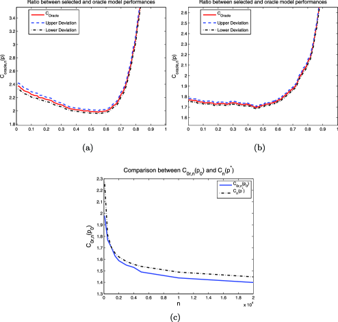
Figure 1: Panels (a) and (b): $p/n\mapsto C_{\mathrm{or},n}(p)$ (plain red line) is plotted for $\Gamma=1$ [see (Dmax)] and different values of $n$: (a) $n=100$, and (b) $n=1000$. $p/n\mapsto C^{+}_{\mathrm{oracle},n}(p)$ (blue dashed line) and $p/n\mapsto C^{-}_{\mathrm{oracle},n}(p)$ (black dot-dashed line) have been plotted on the same graph as well [see (20)]. Panel (c): $n\mapsto C_{\mathrm{or},n}(p_{0})$ (plain blue line) and $n\mapsto C_{n}(p^{*})$ (black dot-dashed line) are displayed. $N=1000$ samples have been drawn from the mixture of Beta distributions (18).

Corollary 3.1 ((Optimizing upper bound)).

With the notation and assumptions of Theorem 3.1, the constant $C_{n}(p)$ is minimized over $p\in\{1,\ldots,\break n-1\}$ for

$$0<\frac{p_{n}^{*}}{n}=1-\frac{1-5\delta_{n}+4\delta_{n}^{2}-({2}/{(n-1)})(3\delta_{n}-4\delta_{n}^{2})+{\delta_{n}}/{(n-1)}}{1+2(1+{1}/{(n-1)})(3\delta_{n}-4\delta_{n}^{2})-\delta_{n}(1+{1}/{(n-1)})}<1.$$

Furthermore, the optimal ratio $p^{*}/n$ is slowly decreasing to 0 as $n$ tends to $+\infty$

$$p^{*}_{n}\sim_{+\infty}10n\delta_{n}\mathop{\longrightarrow}\limits_{n\to+\infty}+\infty.$$ (16)

The proof has ben deferred to Appendix A.1. Corollary 3.1 describes the rate (up to constant) at which $p=p_{n}^{*}$ has to grow with $n$ to achieve finite-sample optimality. In particular $p_{n}^{*}/n$ in (16) is related to $\delta_{n}$ which is strongly connected to the structure of the model collection as explained following Theorem 3.1. A more complex collection leads to a larger $\delta_{n}$ and then to a larger optimal $p_{n}^{*}$. In other words, $p$ must be chosen large enough to balance the overfitting induced by the structure of the model collection. This phenomenon is observed in practice in the simulation experiments of Section 3.1.4 (Figure 2).

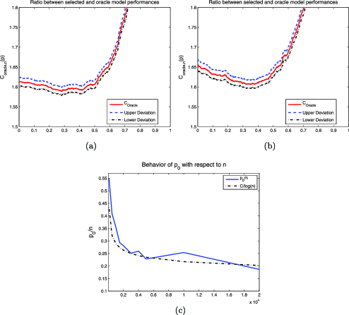
Figure 2: For (a) and (b), $p/n\mapsto C_{\mathrm{or},n}(p)$ (plain red line) is plotted for $n=2000$ and different values of $\Gamma$ [see (Dmax)]: (a) $\Gamma=1$, (b) $\Gamma=2$. $p/n\mapsto C^{+}_{\mathrm{oracle},n}(p)$ (blue dashed line) and $p/n\mapsto C^{-}_{\mathrm{oracle},n}(p)$ (black dot-dashed line) have been plotted on the same graph as well [see (20)]. $N=1000$ samples have been drawn from the mixture of Beta distributions (18). For (c), $n\mapsto p_{0}/n$ (blue plain line) and $n\mapsto C/(\log n)$ (black dot-dashed line) are displayed, where $p_{0}$ denotes the minimizer of $C_{\mathrm{or},n}(p)$ as a function of $p$ and $C$ is a constant.

3.1.3 Adaptivity in the minimax sense

Adaptivity in the minimax sense is a desirable property for model selection procedures. It means the considered procedure automatically adapts to the unknown smoothness of the target function $s$ to estimate [see Barron, Birgé and Massart (1999) for an extensive presentation].

Several adaptivity in the minimax sense results are provided in the present section. Deriving such results from oracle inequalities (1) is somewhat classical. Here, the novelty is first that CV enjoys such a desirable property as a model selection procedure, second that the leading constant $C_{n}(p)$ in Theorem 3.1 when converging to 1 as $n$ tends to $+\infty$ provides accurate results.

Let us start providing a general theorem from which any adaptivity result will be immediate corollary. The proof is given in Appendix A.1.

Theorem 3.2.

Let $s$ denote a density on $[0,1]$ such that (SqI) holds true, set $\{S_{m}\}_{m\in\mathcal{M}_{n}}$ a collection of models defined in Section 2.1.2, and assume (Pol), (RegD), (Dmax), (Rich), (LoEx), (Bias), and (OrSp). Let $\widehat{m}=\widehat{m}(p)$ denote the model minimizing $\widehat{R}_{p}(m)$ over $\mathcal{M}_{n}$ for every $p\in\{1,\ldots,n-1\}$. Then for every $1\leq p\leq n-1$,

$$\mathbb{E}\bigl{[}\|s-\widehat{s}_{\widehat{m}(p)}\|^{2}\bigr{]}$$

(17)

$$\qquad\leq C_{n}(p)\mathbb{E}\Bigl{[}\inf_{m\in\mathcal{M}_{n}}\|s-\widehat{s}_{m}\|^{2}\Bigr{]}+\bigl{(}\Phi+\|s\|^{2}\bigr{)}\frac{12}{n(\log n)^{2}}+\frac{6c_{u}}{n^{2}},$$

where $C_{n}(p)=\frac{T_{B}^{+}\vee T_{V}^{+}}{T_{B}^{-}\wedge T_{V}^{-}}$, with

$$T_{B}^{-} = 1-\delta_{n}K(n,p),$$

$$T_{V}^{-} = \frac{1}{1-p/n}(1-\delta_{n})[1-4\delta_{n}]-2\delta_{n}K(n,p)[3-4\delta_{n}],$$

$$T_{B}^{+} = 1+\delta_{n}K(n,p),$$

$$T_{V}^{+} = \frac{1}{1-p/n}(1+\delta_{n})[1+4\delta_{n}]+2\delta_{n}K(n,p)[3+4\delta_{n}],$$

and $K(n,p)=1+\frac{2}{n-1}+\frac{p}{n-p}\frac{1}{n-1}$.

The last two terms in the right-hand side of (3.2) are remainder terms by Assumptions (RegD), (Dmax), and (Bias).

Applying Theorem 3.2 to the collection of regular histograms defined by (6), the following corollary settles an adaptivity property with respect to Hölder balls [see DeVore and Lorentz (1993)].

Corollary 3.2.

Let us consider the model collection of Section 2.1.2 made of piecewise constant functions and the associated histograms defined by (6) such that, for every $m\in\mathcal{M}_{n}$ and $\lambda\in\Lambda(m)$, $|I_{\lambda}|=D_{m}^{-1}$ (regular histograms). Let us also assume (Dmax) and (LoEx) hold true.

If the target density $s$ belongs to the Hölder ball $\mathcal{H}(L,\alpha)$ for some $L>0$ and $\alpha\in(0,1]$, then there exist constants $0<K_{\alpha}^{-}\leq K_{\alpha}^{+}$ such that for every $p=o(n)$,

$$K_{\alpha}^{-}L^{{2}/{(2\alpha+1)}}n^{-{2\alpha}/{(2\alpha+1)}}$$

$$\qquad\leq\sup_{s\in\mathcal{H}(L,\alpha)}\mathbb{E}\bigl{[}\|s-\widehat{s}_{\widehat{m}(p)}\|^{2}\bigr{]}$$

$$\qquad\leq\bigl{(}1+o(1)\bigr{)}K_{\alpha}^{+}L^{{2}/{(2\alpha+1)}}n^{-{2\alpha}/{(2\alpha+1)}}+O\biggl{(}\frac{1}{n(\log n)^{2}}\biggr{)},$$

$K_{\alpha}^{-}$ and $K_{\alpha}^{+}$ only depend on $\alpha$ (not on $n$ or $s$).

Furthermore, since this property holds for every $L>0$ and $\alpha\in(0,1]$, then $\{\widehat{s}_{\widehat{m}(p)}\}_{n\in\mathbb{N}^{*}}$ is adaptive in the minimax sense with respect to $\{\mathcal{H}(L,\alpha)\}_{L>0,\alpha\in(0,1]}$ for every $p=o(n)$.

The proof has been deferred to Section B.5 in Celisse (2014). The upper bound is tight since the rate $n^{-{2\alpha}/{(2\alpha+1)}}$ and the dependence on the radius $L^{{2}/{(2\alpha+1)}}$ are the same as in the lower bound, which has been stated by Ibragimov and Has’minskiĭ (1981). The main contribution of this result is to prove $p=o(n)$ leads to adaptivity. Note that similar results can also be proved for Besov balls $\mathcal{B}_{\infty,2}^{\alpha}(L)$, with $\alpha,L>0$, for instance [see DeVore and Lorentz (1993)], by using an appropriate collection of models such as trigonometric polynomials defined by (7).

3.1.4 Simulation experiments

Results of simulation experiments are provided to check the conclusions drawn (from theory) in Section 3.1.2. A mixture of Beta distributions

$$\forall x\in[0,1]\qquad s(x)=\frac{\beta(3,7;x)+\beta(10,5;x)}{2}$$ (18)

has been used to generate samples of size $n=100,500,1000,2000,3000,4000,\break 5000,10\mbox{,}000,20\mbox{,}000$. Note that (18) defines a Hölder density on $[0,1]$. For each $n$, every $p\in\{1,\ldots,n-1\}$ have been considered and (Dmax) is fulfilled with $\Gamma=1$ (Figure 1) and $\Gamma=2$ (Figure 2).

The model collection we used is made of piecewise constant functions described in Section 2.1.2 leading to regular histogram estimators defined by (6). Only regular histograms with dimension $D_{m}\geq 2$ are used so that (LoEx) holds true (Lemma B.3). For every $1\leq p\leq n-1$, $\widehat{m}(p)$ is defined by (15).

Let us also introduce

$$\qquad C_{\mathrm{or},n}(p):=\mathbb{E}\biggl{[}\frac{\|s-\widehat{s}_{\widehat{m}(p)}\|^{2}}{\inf_{m\in\mathcal{M}_{n}}\{\|s-\widehat{s}_{m}\|^{2}\}}\biggr{]}\quad\mbox{and}\quad p_{0}:=\mathop{\operatorname{Argmin}}_{1\leq p\leq n-1}C_{\mathrm{or},n}(p),$$ (19)

which measures the average performance of $\widehat{s}_{\widehat{m}(p)}$ with respect to that of $\widehat{s}_{m^{*}}$ (oracle estimator). The closer $C_{\mathrm{or},n}(p)$ to 1, the better $\widehat{s}_{\widehat{m}(p)}$. Minimizing $C_{\mathrm{or},n}(p)$ as a function of $p$ for various values of $n$ enables to check whether the conclusions drawn from minimizing $C_{n}(p)$ with respect to $p$ (Theorem 3.1 and Corollary 3.1) hold true or not, that is whether $C_{n}(p)$ is an accurate approximation to $C_{\mathrm{or},n}(p)$. For each curve $p\mapsto C_{\mathrm{or},n}(p)$, a confidence band has been displayed. It is delimited by $p\mapsto C_{\mathrm{or},n}^{-}(p)$ and $p\mapsto C_{\mathrm{or},n}^{+}(p)$, respectively, defined by

$$C_{\mathrm{or},n}^{-}(p)=C_{\mathrm{or},n}(p)-\frac{\widehat{\sigma}}{\sqrt{N}}\quad\mbox{and}\quad C_{\mathrm{or},n}^{+}(p)=C_{\mathrm{or},n}(p)+\frac{\widehat{\sigma}}{\sqrt{N}},$$ (20)

where $\widehat{\sigma}$ denotes the empirical standard deviation.

First, from panels (a) and (b) of Figure 1, $C_{\mathrm{or},n}(p)$ (plain red lines) decreases pointwise as $n$ grows. This is confirmed by panel (c) of Figure 1 at the particular value $p=p_{0}$ as $n$ grows. This is in accordance with Theorem 3.1 and $C_{n}(p)\to 0$ as $n$ increases. Second, the optimization strategy at the basis of Corollary 3.1 is empirically validated by panel (c) of Figure 1 where $C_{\mathrm{or},n}(p_{0})$ and its proxy $C_{n}(p_{0})$ remain very close to each other. Furthermore, the optimal rate derived in Corollary 3.1 is supported up to constant by simulation results displayed in panel (c) of Figure 2 where $p_{0}/n$ is almost equal to the predicted $\delta_{n}\approx C/(\log n)$ ($C>0$) from the proof of Theorem 3.1.

The conclusion of Corollary 3.1 about the dependence of the optimal $p_{0}$ on the complexity of the model collection (through $\delta_{n}$) is also illustrated by panels (a) and (b) in Figure 2 where $\Gamma$ (Dmax), respectively, equals $1$ and $2$. As $\Gamma$ grows the model collection becomes more complex, leading to a worse performance and a larger $p_{0}$ in panel (b). The need for a larger $p_{0}$ is all the more strong as the curve in panel (b) is less flat than in panel (a), indicating the problem becomes more difficult as $\Gamma$ increases and any misspecification of $p_{0}$ leads to a stronger loss in accuracy. One concludes the more complex the model collection, the larger the optimal $p$.

Note that this conclusion does not apply to Loo ($p=1$) [see (16)], suggesting Loo may be suboptimal for finite sample size. This is supported by Figure 1 [panels (a) and (b)] and Figure 2 [panels (a) and (b)] where the minimum of each curve is not reached at $p=1$.

3.2 Optimal cross-validation for identification

With the notation of Section 2.1, $\{\widehat{s}_{m}\}_{m\in\mathcal{M}_{n}}$ denotes a collection of projection estimators (Section 2.1.2) which is allowed to depend on $n$. The purpose is now to recover the best model denoted by $S_{\bar{m}}$ and defined by

$$\bar{m}:=\mathop{\operatorname{Argmin}}_{m\in\mathcal{M}_{n}}\mathbb{E}\bigl{[}\|s-\widehat{s}_{m}\|^{2}\bigr{]},$$ (21)

where $\bar{m}$ is a deterministic quantity unlike $m^{*}$ from Section 3.1. Since this goal cannot be reached if other models can perform as well as $S_{\bar{m}}$ (even asymptotically), one also requires there exist $\mu>0$ and $n_{0}\in\mathbb{N}^{*}$ such that for every integer $n>n_{0}$,

$$(1+\mu)\mathbb{E}\bigl{[}\|s-\widehat{s}_{\bar{m}}\|^{2}\bigr{]}\leq\inf_{m\in\mathcal{M}_{n}\setminus\{\bar{m}\}}\mathbb{E}\bigl{[}\|s-\widehat{s}_{m}\|^{2}\bigr{]}.$$ (BeMo)

A similar assumption (in probability rather than in expectation) has been made by Yang (2007). Let us further assume the collection $\{S_{m}\}_{m\in\mathcal{M}_{n}}$ can be split into:

• parametric models indexed by $\mathcal{M}_{n,P}$ for which there exist constants $\pi,\tau>0$ (independent of $n$) such that

  $$\sup_{m\in\mathcal{M}_{n,P}}\bigl{\{}n\mathbb{E}\bigl{[}\|s_{m}-\widehat{s}_{m}\|^{2}\bigr{]}\bigr{\}}\leq\pi\quad\mbox{and}\quad\inf_{m\in\mathcal{M}_{n,P},s\notin S_{m}}\bigl{\{}\|s-s_{m}\|^{2}\bigr{\}}\geq\tau.$$ (22)

• nonparametric models indexed by $\mathcal{M}_{n,NP}$ such that

  $$n(\log n)^{-2}\inf_{m\in\mathcal{M}_{n,NP}}\mathbb{E}\bigl{[}\|s_{m}-\widehat{s}_{m}\|^{2}\bigr{]}\mathop{\longrightarrow}\limits_{n\to+\infty}+\infty.$$ (23)

  Then

  $$\{S_{m}\}_{m\in\mathcal{M}_{n}}=\{S_{m}\}_{m\in\mathcal{M}_{n,P}}\cup\{S_{m}\}_{m\in\mathcal{M}_{n,NP}}.$$ (P-NP)

Parametric models are models with convergence rate of order $1/n$. Since $\mathbb{E}[\|s-\widehat{s}_{m}\|^{2}]\approx\|s-s_{m}\|^{2}+C\cdot D_{m}/n$, allowing $D_{m}$ to depend on $n$ makes the rate of the corresponding model slower than $1/n$ (nonparametric model). Consistently with this remark, (22) requires the largest dimension over parametric models is bounded by a constant independent of $n$, and that the bias of parametric models such that $s\notin S_{m}$ cannot decrease with $n$ toward 0. Otherwise, such a model would be nonparametric. Conversely, (23) only requires that the dimension of nonparametric models must be larger than $(\log n)^{2}$. In particular, this does not prevent nonparametric models from containing $s$ or having their bias decreasing to 0 as $n$ grows.

3.2.1 Main results

Depending on whether $s$ belongs or not to $\bigcup_{m\in\mathcal{M}_{n}}S_{m}$, the two following results prove model selection consistency for CV. Their main contribution is to relate the cardinality $p$ of the test set to the rate of convergence of $\widehat{s}_{\bar{m}}$ and the model collection complexity. Note that, in addition, the model consistency property is settled with a collection of models allowed to grow with $n$, which contrasts with earlier results [see, e.g., Yang (2007)].

Let us start with the setting where $s$ belongs to $\bigcup_{m\in\mathcal{M}_{n}}S_{m}$, which implies the best estimator $\widehat{s}_{\bar{m}}$ achieves the parametric rate $1/n$.

Theorem 3.3 ((Model consistency with $s\in\bigcup_{m}S_{m}$)).

Let $\bigcup_{m\in\mathcal{M}_{n}}S_{m}$ denote a collection of models satisfying (Pol) and (P-NP), $\bar{m}\in\mathcal{M}_{n}$ given by (21) be such that (BeMo) holds true, and assume (SqI), (RegD), (Dmax), and (LoEx). For every $1\leq p\leq n-1$, let us also define $\widehat{m}=\widehat{m}(p)=\break\mathop{\operatorname{Argmin}}_{m\in\mathcal{M}_{n}}\widehat{R}_{p}(m)$. If the target $s\in\bigcup_{m\in\mathcal{M}_{n}}S_{m}$, then every $1\leq p=p_{n}\leq n-1$ such that

$$\log(n)\biggl{(}1-\frac{p}{n}\biggr{)}\mathop{\longrightarrow}\limits_{n\to+\infty}0\quad\mbox{and}\quad n\biggl{(}1-\frac{p}{n}\biggr{)}\mathop{\longrightarrow}\limits_{n\to+\infty}+\infty,$$ (24)

leads to

$$\mathbb{P}[\widehat{m}=\bar{m}]\mathop{\longrightarrow}\limits_{n\to+\infty}1.$$

The proof has been deferred to Appendix B.1. When $s$ belongs to $\bigcup_{m\in\mathcal{M}_{n}}S_{m}$, the best estimator $\widehat{s}_{\bar{m}}$ in a polynomial collection can be recovered by CV provided $p/n$ converges to 1 as $n$ tends to $+\infty$. The proof establishes this rate (i) cannot exceed $1/n$ to allow distinguishing between parametric estimators (with convergence rate of order $1/n$), and (ii) has to be faster than $(\log n)^{-1}$ to allow dealing with the polynomial complexity of the model collection. For instance, a finite collection would lead to replace the $(\log n)^{-1}$ rate by a slower one determined by the control level of $\mathbb{P}[\widehat{m}=\bar{m}]$. In the regression setting, [Yang (2007)] already proved requiring $p/n\to 1$ enables to recover the best parametric estimator among parametric ones (see Corollary 1), while this requirement is no longer necessary when comparing parametric and nonparametric estimators. Our result is consistent with Yang’s one, although our setting is somewhat different since we compare the best parametric estimator with both parametric and nonparametric ones in the same time.

Conversely, when $s$ does not belong to $\bigcup_{m}S_{m}$, every parametric model is biased according to (22) and $\widehat{s}_{\bar{m}}$ reaches a nonparametric rate, that is $nR_{n}(\bar{m})\to+\infty$ as $n$ tends to $+\infty$.

Theorem 3.4 ((Model consistency with $s\notin\bigcup_{m}S_{m}$)).

Let $\bigcup_{m\in\mathcal{M}_{n}}S_{m}$ denote a collection of models satisfying (Pol) and (P-NP), $\bar{m}\in\mathcal{M}_{n}$ given by (21) be such that (BeMo) holds true, and assume (SqI), (RegD), (Dmax) and (LoEx). For every $1\leq p\leq n-1$, let us also define $\widehat{m}=\widehat{m}(p)=\break\mathop{\operatorname{Argmin}}_{m\in\mathcal{M}_{n}}\widehat{R}_{p}(m)$. Let us assume the target $s\notin\bigcup_{m\in\mathcal{M}_{n}}S_{m}$ and $R_{n}(\bar{m})\to 0$ as $n$ tends to $+\infty$. [1.]

If for large enough values of $n$ $D_{\bar{m}}\leq(\log n)^{4}$, then every $1\leq p=p_{n}\leq n-1$ such that

$$\log(n)\biggl{(}1-\frac{p}{n}\biggr{)}\mathop{\longrightarrow}\limits_{n\to+\infty}0\quad\mbox{and}\quad n\mathbb{E}\bigl{[}\|s_{\bar{m}}-\widehat{s}_{\bar{m}}\|^{2}\bigr{]}=o(n-p)$$ (25)

leads to

$$\mathbb{P}[\widehat{m}=\bar{m}]\mathop{\longrightarrow}\limits_{n\to+\infty}1.$$

If for large enough values of $n$ $D_{\bar{m}}>(\log n)^{4}$, then every $1\leq p=p_{n}\leq n-1$ such that

$$\frac{(\log n)^{5}}{n\mathbb{E}[\|s_{\bar{m}}-\widehat{s}_{\bar{m}}\|^{2}]} = o\biggl{(}\frac{p/n}{1-p/n}\biggr{)}\quad\mbox{and}$$

$$\frac{p/n}{1-p/n} = o\biggl{(}1\vee\frac{\|s-s_{\bar{m}}\|^{2}}{\mathbb{E}[\|s_{\bar{m}}-\widehat{s}_{\bar{m}}\|^{2}]}\biggr{)}$$

leads to

$$\mathbb{P}[\widehat{m}=\bar{m}]\mathop{\longrightarrow}\limits_{n\to+\infty}1.$$

The proof is similar to that of Theorem 3.3 and has been postponed to Section C.1 [supplementary material Celisse (2014)]. The constraints on $p$ strongly depend on the rate of convergence of $\widehat{s}_{\bar{m}}$ (nonparametric here). When $S_{\bar{m}}$ is a small nonparametric model ($D_{\bar{m}}\leq(\log n)^{4}$), (25) is very similar to (24) in the parametric setting. In particular, $n\mathbb{E}[\|s_{\bar{m}}-\widehat{s}_{\bar{m}}\|^{2}]\to+\infty$ as $n$ tends to $+\infty$ implies $n(1-p/n)\to+\infty$ as well. For large nonparametric models ($D_{\bar{m}}>(\log n)^{4}$), the constraints on $p$ are related to the ratio $\|s-s_{\bar{m}}\|^{2}/\mathbb{E}[\|s_{\bar{m}}-\widehat{s}_{\bar{m}}\|^{2}]$. For instance, when estimating $s\in\mathcal{H}(L,\alpha)$ by regular histograms, this ratio remains bounded while $n\mathbb{E}[\|s_{\bar{m}}-\widehat{s}_{\bar{m}}\|^{2}]$ grows polynomially in $n$. Then $p/n$ has to converge to $0$ as $n$ increases, but not too fast. In particular, Loo ($p=1$) is suboptimal in that setting [see Figure 4 panel (b)]. Note that Theorem 3.4 has the same flavor as Corollary 1 in [Yang (2007)], except the density estimation setting allows to relate $p$ to the features of the best estimator more closely.

3.2.2 Simulation experiments

Simulation experiments have been performed in the settings of Theorems 3.3 and 3.4, respectively, when $s$ belongs to (resp., does not belong to) the model collection. We used a polynomial model collection made of regular piecewise constant functions described in Section 2.1.2 for which Assumptions (P-NP) and (BeMo) are fulfilled with $\mu=5.10^{-1}$. In each setting, $N=1000$ samples have been drawn. Results are given in Figures 3 and 4 where $\mathbb{P}[\widehat{m}=\bar{m}]$ is displayed with respect to the ratio $p/n$. Let us also mention that Lemma B.3 in the supplement Celisse (2014) clearly shows (LoEx) holds true for all densities defined in the following as long as $D_{m}\geq 2$ for every model in the collection.

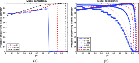
Figure 3: $p/n\mapsto\mathbb{P}[\widehat{m}=\bar{m}]$ for density $s_{1}$ [panel (a)] and $s_{2}$ [panel (b)]. $N=1000$ samples have been drawn.

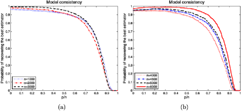
Figure 4: $p/n\mapsto\mathbb{P}[\widehat{m}=\bar{m}]$ for density $s_{3}$ [panel (a)] and $s_{4}$ [panel (b)]. $N=1000$ samples have been drawn.

When $s$ belongs to the model collection (Figure 3), the following densities have been used:

1. $s_{1}(t)=\frac{6}{8}\mathbh{1}_{[0,1/2]}(t)+\frac{10}{8}\mathbh{1}_{[1/2,1]}(t)$, $t\in[0,1]$ [panel (a)],

2. $s_{2}(t)=\frac{135}{112}\mathbh{1}_{[0,1/3]}(t)+\frac{135}{56}\mathbh{1}_{[1/3,1/2]}(t)+\frac{1}{4}\mathbh{1}_{[1/2,5/7]}(t)+\frac{1}{2}\mathbh{1}_{[5/7,1]}(t)$, $t\in[0,1]$ [panel (b)].

As predicted by Theorem 3.3, CV reaches model selection consistency for recovering the best parametric estimator $\widehat{s}_{\bar{m}}$ on condition $p/n$ increases to $1$ as $n$ grows to $+\infty$. Comparing (a) and (b), the convergence rate is slower in (b). Unlike (a) where $\bar{m}$ remains almost unchanged as $n$ increases, the best parametric estimator in (b) changes with $n$ as allowed by (21). Therefore, the slower convergence rate in (b) results from the higher dimension of the space of piecewise constant functions $s_{2}$ belongs to.

When $s$ does not belong to the model collection (Figure 4), densities with different smoothness assumptions have been considered:

1. $s_{3}(x)=\beta(10,7;x)$, for every $t\in[0,1]$ [panel (a)],

2. $s_{4}(x)=\frac{6}{5}x^{1/5}$, for every $t\in[0,1]$ [panel (b)].

The converse situation arises since CV reaches model selection consistency as long as $p/n$ decreases to $0$ as $n$ tends to $+\infty$. Consistently with Theorem 3.4, this rate strongly depends on the risk of the best estimator, that is on the smoothness of the target. While model selection consistency is illustrated by both panels (a) and (b), it is faster for the smoothest density $s_{3}$ than for $s_{4}$. In Figure 4 panel (b), the highest probability is achieved for $p/n\approx 0.18$ with $n=6000$.

4 Discussion

From the present analysis of CV procedures in the density estimation framework, we were able to prove the optimality of leave-one-out cross-validation for risk estimation, which is consistent with earlier results in the regression setting Burman (1989).

However, when CV is used as model selection procedure, the optimal $p$ strongly depends on the structure of the model collection and on our goal (estimation or identification).

Estimation. When the best model has dimension growing with $n$ [faster than $(\log n)^{a}$ for some $a>0$] and the model collection has a polynomial complexity (Pol), Theorem 3.1 proves any $p$ such that $p/n\to 0$ leads to an asymptotically optimal model selection procedure. This is consistent with the asymptotic equivalence between Lpo (as long as $p/n\to 0$) and Mallows’ $C_{p}$ previously settled in the regression setting [Shao (1997)].

From a nonasymptotic point of view, Corollary 3.1 suggests choosing $p>1$ (for finite sample) could balance the overfitting phenomenon arising from selecting a model from a large collection. This overfitting phenomenon is already well known with penalized criteria such as Mallow’s ones, inducing the need for heavier constants in front of the penalty Arlot and Massart (2009). Therefore, increasing $p$ amounts to penalize more strongly complex models (with large dimension).

Identification. As settled by Yang (2007) for regression, Section 3.2 highlights the optimal $p$ depends on the rate of convergence of the estimator one tries to recover (and on the structure of the model collection).

When the target estimator has a parametric rate with a polynomial collection, Theorem 3.3 proves $p/n\to 1$ leads to model selection consistency. This fact has been already noticed by Shao (1993) in the regression setting who proved leave-one-out is not model selection consistent. Remembering the asymptotic equivalence between Lpo and BIC-like criteria [Shao (1997)] established with the linear regression model, this confirms the somewhat paradoxical requirement [Yang (2006)] to devote most of available data ($p>n/2$) to the test set when trying to recover a parametric estimator.

Drawing such a simple conclusion is harder when the best estimator has a nonparametric rate as detailed by Theorem 3.4. If the best estimator has a rate close to parametric, then $p/n\to 1$ provides model selection consistency. Conversely, if the rate is slower (e.g., polynomial of order $n^{-a}$, for some $a>0$), then requiring $p/n\to 0$ enables to recover the target estimator. Relating that way the optimal $p$ to the rate of convergence of the best estimator has been already done in the regression context by [Yang (2007), see Corollary 1].

Note that when the best estimator is nonparametric (e.g., with polynomial rate), Theorem 3.1 and Theorem 3.4 imply $p/n\to 0$ leads to both efficiency and, respectively, model selection consistency. However, there is no contradiction with the earlier paper by Yang (2005) where it was proved no model selection criterion can share both efficiency and model selection consistency in a parametric setting. For instance, Li (1987) has established model selection consistency for leave-one-out with nonparametric estimators in regression.

Appendix A Estimation point of view

A.1 Main proofs

Proof of Theorem 3.1 First, let us use Proposition A.2 from Celisse (2014) applied with $m,m^{\prime}\in\mathcal{M}_{n}$ such that $\widehat{R}_{p}(m^{\prime})\leq\widehat{R}_{p}(m)$. Then it comes

$$\frac{n}{n-p}\mathbb{E}\bigl{[}Z_{m^{\prime}}^{2}\bigr{]}+\|s-s_{m^{\prime}}\|^{2}-K(n,p)\bigl{[}Z_{m^{\prime}}^{2}-\mathbb{E}\bigl{[}Z_{m^{\prime}}^{2}\bigr{]}\bigr{]}$$

$$\qquad\leq\frac{n}{n-p}\mathbb{E}\bigl{[}Z_{m}^{2}\bigr{]}+\|s-s_{m}\|^{2}-K(n,p)\bigl{[}Z_{m}^{2}-\mathbb{E}\bigl{[}Z_{m}^{2}\bigr{]}\bigr{]}$$

$$\qquad\quad{}-2K(n,p)\nu_{n}(s_{m^{\prime}}-s_{m})+\frac{1}{n}\biggl{(}{K(n,p)+\frac{n}{n-p}}\biggr{)}\nu_{n}(\phi_{m^{\prime}}-\phi_{m}),$$

where $K(n,p)=1+\frac{2}{n-1}+\frac{p}{n-p}\frac{1}{n-1}$.

Then, combining Propositions B.4 and B.5 from Celisse (2014) to control the remainder terms, there exist a sequence $(\delta_{n})_{\mathbb{N}}$ with $\delta_{n}\to 0$ and $n\delta_{n}\to+\infty$ as $n\to+\infty$ and an event $\Omega=\Omega_{\mathrm{rem},1}\cap\Omega_{\mathrm{rem},2}$ of probability $1-4/n^{2}$ on which

$$\frac{n}{n-p}\mathbb{E}\bigl{[}Z_{m^{\prime}}^{2}\bigr{]}+\|s-s_{m^{\prime}}\|^{2}-K(n,p)\bigl{[}Z_{m^{\prime}}^{2}-\mathbb{E}\bigl{[}Z_{m^{\prime}}^{2}\bigr{]}\bigr{]}$$

$$\qquad\leq\frac{n}{n-p}\mathbb{E}\bigl{[}Z_{m}^{2}\bigr{]}+\|s-s_{m}\|^{2}-K(n,p)\bigl{[}Z_{m}^{2}-\mathbb{E}\bigl{[}Z_{m}^{2}\bigr{]}\bigr{]}$$

$$\qquad\quad{}+\delta_{n}K(n,p)\bigl{(}\|s-s_{m^{\prime}}\|^{2}+\mathbb{E}\bigl{[}Z_{m^{\prime}}^{2}\bigr{]}+\|s-s_{m}\|^{2}+\mathbb{E}\bigl{[}Z_{m}^{2}\bigr{]}\bigr{)}$$

$$\qquad\quad{}+\delta_{n}\biggl{(}{K(n,p)+\frac{n}{n-p}}\biggr{)}\bigl{[}\mathbb{E}\bigl{[}Z_{m^{\prime}}^{2}\bigr{]}+\mathbb{E}\bigl{[}Z_{m}^{2}\bigr{]}\bigr{]}.$$

In the following, $\delta_{n}$ always denotes such a sequence even if the precise expression of $\delta_{n}$ can differ from line to line.

Let us now use concentration results stated in Corollaries B.1 and B.2 from Celisse (2014) on the events $\Omega_{\mathrm{left}}$ and $\Omega_{\mathrm{right}}$. The important point in this proof is given by Lemmas B.1 and B [Celisse (2014)], where it is proved that on the event $\Omega=\Omega_{\mathrm{left}}\cap\Omega_{\mathrm{right}}\cap\Omega_{\mathrm{rem},1}\cap\Omega_{\mathrm{rem},1}$, $\min\{D_{m^{*}},D_{\widehat{m}(p)}\}\geq(\log n)^{4}$ for large enough values of $n$. Therefore, one can apply Lemma B.6 and Corollaries B.1 and B.2 from Celisse (2014) with $L_{m}=0=r_{n}(m)$ to get

$$Z_{m^{\prime}}^{2}\biggl{[}\biggl{(}\frac{n}{n-p}(1-\delta_{n})-2\delta_{n}K(n,p)\biggr{)}(1-4\delta_{n})-4K(n,p)\delta_{n}\biggr{]}$$

$$\quad{}+\bigl{[}1-\delta_{n}K(n,p)\bigr{]}\|s-s_{m^{\prime}}\|^{2}$$

$$\qquad\leq Z_{m}^{2}\biggl{[}\biggl{(}\frac{n}{n-p}(1+\delta_{n})+2\delta_{n}K(n,p)\biggr{)}(1+4\delta_{n})+4K(n,p)\delta_{n}\biggr{]}$$

$$\qquad\quad{}+\bigl{[}1+\delta_{n}K(n,p)\bigr{]}\|s-s_{m}\|^{2}.$$

Choosing $m^{\prime}=\widehat{m}$, it comes

$$T_{V}^{-}Z_{\widehat{m}}^{2}+T_{B}^{-}\|s-s_{\widehat{m}}\|^{2}\leq T_{V}^{+}Z_{m}^{2}+T_{B}^{+}\|s-s_{m}\|^{2},$$

where

$$T_{B}^{-} = 1-\delta_{n}K(n,p),$$

$$T_{V}^{-} = \frac{n}{n-p}(1-\delta_{n})[1-4\delta_{n}]-2K(n,p)\bigl{[}3\delta_{n}-4\delta_{n}^{2}\bigr{]},$$

$$T_{B}^{+} = 1+\delta_{n}K(n,p),$$

$$T_{V}^{+} = \frac{n}{n-p}(1+\delta_{n})[1+4\delta_{n}]+2K(n,p)\bigl{[}3\delta_{n}+4\delta_{n}^{2}\bigr{]}.$$

Finally on the event $\Omega$, the following oracle inequality holds true for every $p\in\{1,n-1\}$:

$$\|s-\widehat{s}_{\widehat{m}(p)}\|^{2}\leq C_{n}(p)\inf_{m\in\mathcal{M}_{n}}\bigl{\{}\|s-\widehat{s}_{m}\|^{2}\bigr{\}}\qquad\mbox{with }C_{n}(p)=\frac{T_{B}^{+}\vee T_{V}^{+}}{T_{B}^{-}\wedge T_{V}^{-}}.$$

Moreover, on the event $\Omega$, Lemmas B.1 and B.2 [Celisse (2014)] show $\min\{D_{m^{*}},D_{\widehat{m}(p)}\}\geq(\log n)^{4}$. Then, it is enough to apply Propositions B.1 and B.2 from Celisse (2014) to models satisfying this constraint, which leads to the new event $\widetilde{\Omega}$ [where models with dimension smaller than $(\log n)^{4}$ have been omitted] of probability at least $1-6/n^{2}$.

Proof of Corollary 3.1 Let us recall the expression of the leading constant

$$C_{n}(p)=\frac{T_{B}^{+}\vee T_{V}^{+}}{T_{B}^{-}\wedge T_{V}^{-}},$$

with

$$T_{B}^{-} = 1-\delta_{n}K(n,p),$$

$$T_{V}^{-} = \frac{1}{1-p/n}(1-\delta_{n})[1-4\delta_{n}]-2\delta_{n}K(n,p)[3-4\delta_{n}],$$

$$T_{B}^{+} = 1+\delta_{n}K(n,p),$$

$$T_{V}^{+} = \frac{1}{1-p/n}(1+\delta_{n})[1+4\delta_{n}]+2\delta_{n}K(n,p)[3+4\delta_{n}],$$

and $K(n,p)=1+\frac{2}{n-1}+\frac{p}{n-p}\frac{1}{n-1}$.

First, as long as $n$ is large enough, simple calculations when $p=1$ show $T_{V}^{-}(1)\leq T_{B}^{-}(1)$. Noticing moreover that $T_{V}^{+}(p)\geq T_{B}^{+}(p)$ for every $p$, it comes for $p$ close to 1

$$C_{n}(p)=\frac{T_{V}^{+}}{T_{V}^{-}}=\frac{(1+\delta_{n})[1+4\delta_{n}]+2(1-p/n)\delta_{n}K(n,p)[3+4\delta_{n}]}{(1-\delta_{n})[1-4\delta_{n}]-2(1-p/n)\delta_{n}K(n,p)[3-4\delta_{n}]}.$$

It is then easy to show that $p\mapsto C_{n}(p)$ is decreasing on $\{1,\ldots,p^{*}\}$, where $p^{*}$ denotes the value of $p$ such that $T_{V}^{-}(p)=T_{B}^{-}(p)$. Hence,

$$\frac{p_{n}^{*}}{n}=1-\frac{1-5\delta_{n}+4\delta_{n}^{2}-({2}/{(n-1)})(3\delta_{n}-4\delta_{n}^{2})+{\delta_{n}}/{(n-1)}}{1+2(1+{1}/{(n-1)})(3\delta_{n}-4\delta_{n}^{2})-\delta_{n}(1+{1}/{(n-1)})}.$$

It results that for every $p\geq p^{*}$

$$C_{n}(p)=\frac{T_{V}^{+}}{T_{B}^{-}},$$

which is increasing with respect to $p$.

In the same way, it is easy to check that $p_{n}^{*}/(10n\delta_{n})\mathop{\longrightarrow}\limits_{n\to+\infty}1$, which enables us to conclude the proof.

Proof of Theorem 3.2 Introducing the event $\widetilde{\Omega}$ of Theorem 3.1, we get

$$\mathbb{E}\bigl{[}\|s-\widehat{s}_{\widehat{m}(p)}\|^{2}\bigr{]}=\mathbb{E}\bigl{[}\|s-\widehat{s}_{\widehat{m}(p)}\|^{2}\mathbh{1}_{\widetilde{\Omega}}\bigr{]}+\mathbb{E}\bigl{[}\|s-\widehat{s}_{\widehat{m}(p)}\|^{2}\mathbh{1}_{\widetilde{\Omega}^{c}}\bigr{]}.$$

Then Theorem 3.1 applied to the first expectation in the right-hand side leads to

$$\mathbb{E}\bigl{[}\|s-\widehat{s}_{\widehat{m}(p)}\|^{2}\bigr{]}\leq C_{n}(p)\mathbb{E}\Bigl{[}\inf_{m\in\mathcal{M}_{n}}\|s-\widehat{s}_{m}\|^{2}\Bigr{]}+\mathbb{E}\bigl{[}\|s-\widehat{s}_{\widehat{m}(p)}\|^{2}\mathbh{1}_{\widetilde{\Omega}^{c}}\bigr{]}.$$

Applying (Bias), one gets

$$\mathbb{E}\bigl{[}\|s-s_{\widehat{m}(p)}\|^{2}\mathbh{1}_{\widetilde{\Omega}^{c}}\bigr{]}\leq\mathbb{E}\biggl{[}\frac{c_{u}}{D_{\widehat{m}(p)}^{u}}\mathbh{1}_{\widetilde{\Omega}^{c}}\biggr{]}\leq c_{u}\mathbb{P}\bigl{(}\widetilde{\Omega}^{c}\bigr{)}\leq\frac{6c_{u}}{n^{2}},$$

while (RegD) and (Dmax) provide

$$\mathbb{E}\bigl{[}\|s_{\widehat{m}(p)}-\widehat{s}_{\widehat{m}(p)}\|^{2}\mathbh{1}_{\widetilde{\Omega}^{c}}\bigr{]}$$

$$\qquad=\mathbb{E}\biggl{[}\sum_{\lambda\in\Lambda(\widehat{m}(p))}(P_{n}\varphi_{\lambda}-P\varphi_{\lambda})^{2}\mathbh{1}_{\widetilde{\Omega}^{c}}\biggr{]}$$

$$\qquad\leq 2\mathbb{E}\biggl{[}\sum_{\lambda\in\Lambda(\widehat{m}(p))}(P_{n}\varphi_{\lambda})^{2}\mathbh{1}_{\widetilde{\Omega}^{c}}\biggr{]}+2\mathbb{E}\biggl{[}\sum_{\lambda\in\Lambda(\widehat{m}(p))}(P\varphi_{\lambda})^{2}\mathbh{1}_{\widetilde{\Omega}^{c}}\biggr{]}$$

$$\qquad\leq 2\mathbb{E}\Biggl{[}\sum_{\lambda\in\Lambda(\widehat{m}(p))}\frac{1}{n^{2}}\sum_{i,j=1}^{n}\varphi_{\lambda}(X_{i})\varphi_{\lambda}(X_{j})\mathbh{1}_{\widetilde{\Omega}^{c}}\Biggr{]}+2\|s\|^{2}\mathbb{E}[D_{\widehat{m}(p)}\mathbh{1}_{\widetilde{\Omega}^{c}}]$$

$$\qquad\leq 2\bigl{(}\Phi+\|s\|^{2}\bigr{)}\frac{n}{(\log n)^{2}}\mathbb{P}\bigl{(}\widetilde{\Omega}^{c}\bigr{)}\leq\bigl{(}\Phi+\|s\|^{2}\bigr{)}\frac{12}{n(\log n)^{2}}.$$

Appendix B Identification point of view

B.1 Proof of Theorem 3.3

The general purpose is to prove there exist an event $\Omega_{n}$ with $\mathbb{P}(\Omega_{n})\to 1$ as $n$ tends to $+\infty$ and a positive integer $N$ such that on $\Omega_{n}$, for every $n\geq N$, every $m\neq\bar{m}$ satisfies

$$\widehat{R}_{p}(\bar{m})-\widehat{R}_{p}(m)\leq-u_{n}(m)\bigl{(}1+o(1)\bigr{)},$$ (27)

where $u_{n}(m)>0$ denotes a real number for every $n$ and $m$, and $o(1)$ does not depend on $m$. In particular, this implies

$$\mathbb{P}(\widehat{m}=\bar{m})=\mathbb{P}\bigl{(}\forall m\neq\bar{m},\widehat{R}_{p}(\bar{m})-\widehat{R}_{p}(m)<0\bigr{)}\mathop{\longrightarrow}\limits_{n\to+\infty}1,$$ (28)

which would complete the proof.

Let us consider the event $\Omega_{\mathrm{left}}\cap\Omega_{\mathrm{right}}$ in Proposition C.2 from Celisse (2014) with $\beta_{1}=\beta_{2}=1/n^{2}$, and the events $\Omega_{\mathrm{rem},1}$ [Proposition B.4 from Celisse (2014)] and $\Omega_{\mathrm{rem},3}$ (Proposition C.1 [Celisse (2014)]). Then with $\Omega_{n}=\Omega_{\mathrm{left}}\cap\Omega_{\mathrm{right}}\cap\Omega_{\mathrm{rem},1}\cap\Omega_{\mathrm{rem},3}$ and $\mathbb{P}[\Omega_{n}^{c}]\leq 8/n^{2}$, showing (28) amounts to prove

$$\mathbb{P}\bigl{(}\Omega_{n}\cap\bigl{\{}\forall m\neq\bar{m},\widehat{R}_{p}(\bar{m})-\widehat{R}_{p}(m)<0\bigr{\}}\bigr{)}\mathop{\longrightarrow}\limits_{n\to+\infty}1.$$

Let us now focus on the event $\Omega_{n}$. The two main steps correspond to distinguishing between parametric and nonparametric models $S_{m}$ [see (P-NP)]. For every $m$, let us define $B(m)=\|s-s_{m}\|^{2}$ and $V(m)=\mathbb{E}[\|s_{m}-\widehat{s}_{m}\|^{2}]$, where $s_{m}=\mathop{\operatorname{Argmin}}_{t\in S_{m}}\|s-t\|^{2}$. From line to line, the value of $\delta_{n}$ may change, but it always denotes a sequence decreasing to $0$ and such that $n\delta_{n}\to+\infty$ as $n$ grows.

If $\widehat{s}_{m}$ has a parametric rate.

• If $s\in S_{m}$:

  Let us first notice $s_{m}=s=s_{\bar{m}}$, which implies $R_{n}(m)=V(m)$ and $R_{n}(\bar{m})=V(\bar{m})$. Then Proposition A.2 from Celisse (2014), and Propositions B.4 and C.2 from Celisse (2014) lead to

  $$\biggl{|}\bigl{[}\widehat{R}_{p}(\bar{m})-\widehat{R}_{p}(m)\bigr{]}-\frac{n}{n-p}\bigl{[}R_{n}(\bar{m})-R_{n}(m)\bigr{]}\biggr{|}$$

  $$\qquad\leq\biggl{(}36L_{n}^{2}+3\delta_{n}+\delta_{n}\frac{n}{n-p}\biggr{)}\bigl{[}R_{n}(m)+R_{n}(\bar{m})\bigr{]}$$

  $$\qquad=o\biggl{(}\frac{n}{n-p}\biggr{)}\bigl{[}R_{n}(m)+R_{n}(\bar{m})\bigr{]},$$

  by requiring $L_{n}^{2}=o((1-p/n)^{-1})$, which provides (27) by use of (BeMo). Note that in the previous inequality, $r_{n}(\bar{m})$ and $r_{n}(m)$ [from Proposition C.2 from Celisse (2014)] have been omitted since they are negligible with respect to the other terms.

• If $s\notin S_{m}$:

  Similarly, Proposition A.2, Proposition B.4, and Propositions C.1 and C.2 from Celisse (2014) lead to

  $$\biggl{|}\bigl{[}\widehat{R}_{p}(\bar{m})-\widehat{R}_{p}(m)\bigr{]}-\bigl{[}B(\bar{m})-B(m)\bigr{]}-\frac{n}{n-p}\bigl{[}V(\bar{m})-V(m)\bigr{]}\biggr{|}$$

  $$\qquad\leq 6\delta_{n}\bigl{[}B(\bar{m})+B(m)\bigr{]}$$

  $$\qquad\quad{}+\biggl{(}36L_{n}^{2}+3\delta_{n}\frac{\Phi}{\xi}+\delta_{n}\biggl{(}3+\frac{n}{n-p}\biggr{)}\biggr{)}\bigl{[}V(m)+V(\bar{m})\bigr{]}$$

  $$\qquad\quad{}+3\delta_{n}\|s\|\sqrt{\frac{\Phi}{\xi}}\sqrt{V(\bar{m})+V(m)}+r_{n}(\bar{m}).$$

  With $s\in\bigcup_{m^{\prime}}S_{m^{\prime}}$ and $s\notin S_{m}$, it comes $B(\bar{m})=0$ and $B(m)\geq\tau>0$ by (P-NP). Since both $\widehat{s}_{m}$ and $\widehat{s}_{\bar{m}}$ have parametric rates, requiring $n(1-p/n)\to+\infty$ as $n$ grows implies (27), that is,

  $$\bigl{[}\widehat{R}_{p}(\bar{m})-\widehat{R}_{p}(m)\bigr{]}\leq-B(m)\bigl{(}1+o(1)\bigr{)}.$$

If $\widehat{s}_{m}$ has a nonparametric rate.

• If $s\in S_{m}$:

  Proposition A.2 from Celisse (2014), $s_{m}=s=s_{\bar{m}}$, and Propositions C.1 and C.2 from Celisse (2014) combined with $L_{n}^{2}=o(n/(n-p))$ provide

  $$\biggl{|}\bigl{[}\widehat{R}_{p}(\bar{m})-\widehat{R}_{p}(m)\bigr{]}-\frac{n}{n-p}\bigl{[}V(\bar{m})-V(m)\bigr{]}\biggr{|}$$

  $$\qquad\leq o\biggl{(}\frac{n}{n-p}\biggr{)}V(m)+o\biggl{(}\frac{n}{n-p}\biggr{)}V(\bar{m}),$$

  where $o(n/(n-p))$ does not depend on $m$. Since $S_{m}$ is nonparametric, (P-NP) gives

  $$\frac{V(\bar{m})}{V(m)}\leq\frac{\pi}{(\log n)^{2}}\Bigl{(}n/(\log n)^{2}\inf_{m}V(m)\Bigr{)}^{-1}\mathop{\longrightarrow}\limits_{n\to+\infty}0,$$

  which implies (27) with

  $$(n-p)\bigl{[}\widehat{R}_{p}(\bar{m})-\widehat{R}_{p}(m)\bigr{]}\leq-nV(m)\bigl{(}1+o(1)\bigr{)}.$$

• If $s\notin S_{m}$:

  Both $L_{n}^{2}=o(n/(n-p))$ and the same argument as above lead to

  $$\biggl{|}\bigl{[}\widehat{R}_{p}(\bar{m})-\widehat{R}_{p}(m)\bigr{]}+B(m)+\frac{n}{n-p}V(m)\bigl{[}1+o(1)\bigr{]}\biggr{|}$$

  $$\qquad\leq V(m)o\biggl{(}\frac{n}{n-p}\biggr{)}+B(m)o(1).$$

  Then (27) holds true with

  $$\bigl{[}\widehat{R}_{p}(\bar{m})-\widehat{R}_{p}(m)\bigr{]}\leq-B(m)\bigl{(}1+o(1)\bigr{)}-\frac{n}{n-p}V(m)\bigl{(}1+o(1)\bigr{)}.$$

Then there exists an integer $N$ such that for $n\geq N$, on the event $\Omega_{n}$, (27) holds true for every $m\in\mathcal{M}_{n}$, which completes the proof.

References

- Akaike (1973) {bincollection}[mr] \bauthor\bsnmAkaike, \bfnmH.\binitsH. (\byear1973). \btitleInformation theory and an extension of the maximum likelihood principle. In \bbooktitleSecond International Symposium on Information Theory (Tsahkadsor, 1971) \bpages267–281. \bpublisherAkadémiai Kiadó, \blocationBudapest. \bidmr=0483125 \bptokimsref\endbibitem
- Arlot (2007) {bincollection}[auto:STB—2014/06/18—12:29:53] \bauthor\bsnmArlot, \bfnmS.\binitsS. (\byear2007). \btitle-fold penalization: An alternative to -fold cross-validation. In \bbooktitleOberwolfach Reports, Volume 4 of Mathematisches Forschungsinstitut. \bpublisherEMS, \blocationZürich. \bptokimsref\endbibitem
- Arlot and Celisse (2010) {barticle}[mr] \bauthor\bsnmArlot, \bfnmSylvain\binitsS. and \bauthor\bsnmCelisse, \bfnmAlain\binitsA. (\byear2010). \btitleA survey of cross-validation procedures for model selection. \bjournalStat. Surv. \bvolume4 \bpages40–79. \biddoi=10.1214/09-SS054, issn=1935-7516, mr=2602303 \bptokimsref\endbibitem
- Arlot and Celisse (2011) {barticle}[mr] \bauthor\bsnmArlot, \bfnmSylvain\binitsS. and \bauthor\bsnmCelisse, \bfnmAlain\binitsA. (\byear2011). \btitleSegmentation of the mean of heteroscedastic data via cross-validation. \bjournalStat. Comput. \bvolume21 \bpages613–632. \biddoi=10.1007/s11222-010-9196-x, issn=0960-3174, mr=2826696 \bptokimsref\endbibitem
- Arlot and Massart (2009) {barticle}[auto:STB—2014/06/18—12:29:53] \bauthor\bsnmArlot, \bfnmS.\binitsS. and \bauthor\bsnmMassart, \bfnmP.\binitsP. (\byear2009). \btitleData-driven calibration of penalties for least-squares regression. \bjournalJournal of Machine Learning \bvolume10 \bpages245–279. \bptokimsref\endbibitem
- Baraud, Giraud and Huet (2009) {barticle}[mr] \bauthor\bsnmBaraud, \bfnmYannick\binitsY., \bauthor\bsnmGiraud, \bfnmChristophe\binitsC. and \bauthor\bsnmHuet, \bfnmSylvie\binitsS. (\byear2009). \btitleGaussian model selection with an unknown variance. \bjournalAnn. Statist. \bvolume37 \bpages630–672. \biddoi=10.1214/07-AOS573, issn=0090-5364, mr=2502646 \bptokimsref\endbibitem
- Barron, Birgé and Massart (1999) {barticle}[mr] \bauthor\bsnmBarron, \bfnmAndrew\binitsA., \bauthor\bsnmBirgé, \bfnmLucien\binitsL. and \bauthor\bsnmMassart, \bfnmPascal\binitsP. (\byear1999). \btitleRisk bounds for model selection via penalization. \bjournalProbab. Theory Related Fields \bvolume113 \bpages301–413. \biddoi=10.1007/s004400050210, issn=0178-8051, mr=1679028 \bptokimsref\endbibitem
- Barron and Cover (1991) {barticle}[mr] \bauthor\bsnmBarron, \bfnmAndrew R.\binitsA. R. and \bauthor\bsnmCover, \bfnmThomas M.\binitsT. M. (\byear1991). \btitleMinimum complexity density estimation. \bjournalIEEE Trans. Inform. Theory \bvolume37 \bpages1034–1054. \biddoi=10.1109/18.86996, issn=0018-9448, mr=1111806 \bptokimsref\endbibitem
- Bartlett, Boucheron and Lugosi (2002) {barticle}[auto:STB—2014/06/18—12:29:53] \bauthor\bsnmBartlett, \bfnmP.\binitsP., \bauthor\bsnmBoucheron, \bfnmS.\binitsS. and \bauthor\bsnmLugosi, \bfnmG.\binitsG. (\byear2002). \btitleModel selection and error estimation. \bjournalMachine Learning \bvolume48 \bpages85–113. \bptokimsref\endbibitem
- Birgé and Massart (1997) {bincollection}[mr] \bauthor\bsnmBirgé, \bfnmLucien\binitsL. and \bauthor\bsnmMassart, \bfnmPascal\binitsP. (\byear1997). \btitleFrom model selection to adaptive estimation. In \bbooktitleFestschrift for Lucien Le Cam (\beditor\binitsD.\bfnmD. \bsnmPollard, \beditor\binitsE.\bfnmE. \bsnmTorgensen and \beditor\binitsG.\bfnmG. \bsnmYang, eds.) \bpages55–87. \bpublisherSpringer, \blocationNew York. \bidmr=1462939 \bptokimsref\endbibitem
- Birgé and Massart (2001) {barticle}[mr] \bauthor\bsnmBirgé, \bfnmLucien\binitsL. and \bauthor\bsnmMassart, \bfnmPascal\binitsP. (\byear2001). \btitleGaussian model selection. \bjournalJ. Eur. Math. Soc. (JEMS) \bvolume3 \bpages203–268. \biddoi=10.1007/s100970100031, issn=1435-9855, mr=1848946 \bptokimsref\endbibitem
- Birgé and Massart (2007) {barticle}[mr] \bauthor\bsnmBirgé, \bfnmLucien\binitsL. and \bauthor\bsnmMassart, \bfnmPascal\binitsP. (\byear2007). \btitleMinimal penalties for Gaussian model selection. \bjournalProbab. Theory Related Fields \bvolume138 \bpages33–73. \biddoi=10.1007/s00440-006-0011-8, issn=0178-8051, mr=2288064 \bptnotecheck year \bptokimsref\endbibitem
- Birgé and Rozenholc (2006) {barticle}[mr] \bauthor\bsnmBirgé, \bfnmLucien\binitsL. and \bauthor\bsnmRozenholc, \bfnmYves\binitsY. (\byear2006). \btitleHow many bins should be put in a regular histogram. \bjournalESAIM Probab. Stat. \bvolume10 \bpages24–45 (electronic). \biddoi=10.1051/ps:2006001, issn=1292-8100, mr=2197101 \bptokimsref\endbibitem
- Blanchard and Massart (2006) {barticle}[mr] \bauthor\bsnmBlanchard, \bfnmGilles\binitsG. and \bauthor\bsnmMassart, \bfnmPascal\binitsP. (\byear2006). \btitleDiscussion: “Local Rademacher complexities and oracle inequalities in risk minimization” [Ann. Statist. 34 (2006) 2593–2656] by V. Koltchinskii. \bjournalAnn. Statist. \bvolume34 \bpages2664–2671. \biddoi=10.1214/009053606000001037, issn=0090-5364, mr=2329460 \bptokimsref\endbibitem
- Bowman (1984) {barticle}[mr] \bauthor\bsnmBowman, \bfnmAdrian W.\binitsA. W. (\byear1984). \btitleAn alternative method of cross-validation for the smoothing of density estimates. \bjournalBiometrika \bvolume71 \bpages353–360. \biddoi=10.1093/biomet/71.2.353, issn=0006-3444, mr=0767163 \bptokimsref\endbibitem
- Breiman et al. (1984) {bbook}[mr] \bauthor\bsnmBreiman, \bfnmLeo\binitsL., \bauthor\bsnmFriedman, \bfnmJerome H.\binitsJ. H., \bauthor\bsnmOlshen, \bfnmRichard A.\binitsR. A. and \bauthor\bsnmStone, \bfnmCharles J.\binitsC. J. (\byear1984). \btitleClassification and Regression Trees. \bpublisherWadsworth, \blocationBelmont, CA. \bidmr=0726392 \bptokimsref\endbibitem
- Burman (1989) {barticle}[mr] \bauthor\bsnmBurman, \bfnmPrabir\binitsP. (\byear1989). \btitleA comparative study of ordinary cross-validation, -fold cross-validation and the repeated learning-testing methods. \bjournalBiometrika \bvolume76 \bpages503–514. \biddoi=10.1093/biomet/76.3.503, issn=0006-3444, mr=1040644 \bptokimsref\endbibitem
- Burman (1990) {barticle}[mr] \bauthor\bsnmBurman, \bfnmPrabir\binitsP. (\byear1990). \btitleEstimation of optimal transformations using -fold cross validation and repeated learning-testing methods. \bjournalSankhyā Ser. A \bvolume52 \bpages314–345. \bidissn=0581-572X, mr=1178041 \bptokimsref\endbibitem
- Castellan (1999) {bmisc}[auto:STB—2014/06/18—12:29:53] \bauthor\bsnmCastellan, \bfnmG.\binitsG. (\byear1999). \bhowpublishedModified Akaike’s criterion for histogram density estimation. Technical Report 99.61, Univ. Paris-Sud. \bptokimsref\endbibitem
- Castellan (2003) {barticle}[mr] \bauthor\bsnmCastellan, \bfnmGwénaëlle\binitsG. (\byear2003). \btitleDensity estimation via exponential model selection. \bjournalIEEE Trans. Inform. Theory \bvolume49 \bpages2052–2060. \biddoi=10.1109/TIT.2003.814485, issn=0018-9448, mr=2004713 \bptokimsref\endbibitem
- Celisse (2014) {bmisc}[author] \bauthor\bsnmCelisse, \binitsA. (\byear2014). \bhowpublishedSupplement to “Optimal cross-validation in density estimation with the -loss.” DOI:\doiurl10.1214/14-AOS1240SUPP. \bptokimsref \endbibitem
- Celisse and Robin (2008) {barticle}[mr] \bauthor\bsnmCelisse, \bfnmAlain\binitsA. and \bauthor\bsnmRobin, \bfnmStéphane\binitsS. (\byear2008). \btitleNonparametric density estimation by exact leave--out cross-validation. \bjournalComput. Statist. Data Anal. \bvolume52 \bpages2350–2368. \biddoi=10.1016/j.csda.2007.10.002, issn=0167-9473, mr=2411944 \bptokimsref\endbibitem
- DeVore and Lorentz (1993) {bbook}[mr] \bauthor\bsnmDeVore, \bfnmRonald A.\binitsR. A. and \bauthor\bsnmLorentz, \bfnmGeorge G.\binitsG. G. (\byear1993). \btitleConstructive Approximation. \bseriesGrundlehren der Mathematischen Wissenschaften \bvolume303. \bpublisherSpringer, \blocationBerlin. \biddoi=10.1007/978-3-662-02888-9, mr=1261635 \bptokimsref\endbibitem
- Geisser (1974) {barticle}[mr] \bauthor\bsnmGeisser, \bfnmSeymour\binitsS. (\byear1974). \btitleA predictive approach to the random effect model. \bjournalBiometrika \bvolume61 \bpages101–107. \bidissn=0006-3444, mr=0418322 \bptokimsref\endbibitem
- Geisser (1975) {barticle}[auto:STB—2014/06/18—12:29:53] \bauthor\bsnmGeisser, \bfnmS.\binitsS. (\byear1975). \btitleThe predictive sample reuse method with applications. \bjournalJ. Amer. Statist. Assoc. \bvolume70 \bpages320–328. \bptokimsref\endbibitem
- Ibragimov and Has’minskiĭ (1981) {bbook}[mr] \bauthor\bsnmIbragimov, \bfnmI. A.\binitsI. A. and \bauthor\bsnmHas’minskiĭ, \bfnmR. Z.\binitsR. Z. (\byear1981). \btitleStatistical Estimation: Asymptotic Theory. \bseriesApplications of Mathematics \bvolume16. \bpublisherSpringer, \blocationBerlin. \bidmr=0620321 \bptokimsref\endbibitem
- Larson (1931) {barticle}[auto:STB—2014/06/18—12:29:53] \bauthor\bsnmLarson, \bfnmS. C.\binitsS. C. (\byear1931). \btitleThe shrinkage of the coefficient of multiple correlation. \bjournalJ. Educ. Psychol. \bvolume22 \bpages45–55. \bptokimsref\endbibitem
- Ledoux (2001) {bbook}[mr] \bauthor\bsnmLedoux, \bfnmMichel\binitsM. (\byear2001). \btitleThe Concentration of Measure Phenomenon. \bseriesMathematical Surveys and Monographs \bvolume89. \bpublisherAmer. Math. Soc., \blocationProvidence, RI. \bidmr=1849347 \bptokimsref\endbibitem
- Li (1987) {barticle}[mr] \bauthor\bsnmLi, \bfnmKer-Chau\binitsK.-C. (\byear1987). \btitleAsymptotic optimality for , , cross-validation and generalized cross-validation: Discrete index set. \bjournalAnn. Statist. \bvolume15 \bpages958–975. \biddoi=10.1214/aos/1176350486, issn=0090-5364, mr=0902239 \bptokimsref\endbibitem
- Lugosi and Nobel (1999) {barticle}[mr] \bauthor\bsnmLugosi, \bfnmGábor\binitsG. and \bauthor\bsnmNobel, \bfnmAndrew B.\binitsA. B. (\byear1999). \btitleAdaptive model selection using empirical complexities. \bjournalAnn. Statist. \bvolume27 \bpages1830–1864. \biddoi=10.1214/aos/1017939242, issn=0090-5364, mr=1765619 \bptokimsref\endbibitem
- Mallows (1973) {barticle}[auto:STB—2014/06/18—12:29:53] \bauthor\bsnmMallows, \bfnmC. L.\binitsC. L. (\byear1973). \btitleSome comments on . \bjournalTechnometrics \bvolume15 \bpages661–675. \bptokimsref\endbibitem
- Mosteller and Tukey (1968) {bincollection}[auto:STB—2014/06/18—12:29:53] \bauthor\bsnmMosteller, \bfnmF.\binitsF. and \bauthor\bsnmTukey, \bfnmJ. W.\binitsJ. W. (\byear1968). \btitleData analysis, including statistics. In \bbooktitleHandbook of Social Psychology, Vol. 2 (\beditor\bfnmG.\binitsG. \bsnmLindzey and \beditor\bfnmE.\binitsE. \bsnmAronson, eds.). \bpublisherAddison-Wesley, \blocationNew York. \bptokimsref\endbibitem
- Rudemo (1982) {barticle}[mr] \bauthor\bsnmRudemo, \bfnmMats\binitsM. (\byear1982). \btitleEmpirical choice of histograms and kernel density estimators. \bjournalScand. J. Stat. \bvolume9 \bpages65–78. \bidissn=0303-6898, mr=0668683 \bptokimsref\endbibitem
- Schwarz (1978) {barticle}[mr] \bauthor\bsnmSchwarz, \bfnmGideon\binitsG. (\byear1978). \btitleEstimating the dimension of a model. \bjournalAnn. Statist. \bvolume6 \bpages461–464. \bidissn=0090-5364, mr=0468014 \bptokimsref\endbibitem
- Shao (1993) {barticle}[mr] \bauthor\bsnmShao, \bfnmJun\binitsJ. (\byear1993). \btitleLinear model selection by cross-validation. \bjournalJ. Amer. Statist. Assoc. \bvolume88 \bpages486–494. \bidissn=0162-1459, mr=1224373 \bptokimsref\endbibitem
- Shao (1997) {barticle}[mr] \bauthor\bsnmShao, \bfnmJun\binitsJ. (\byear1997). \btitleAn asymptotic theory for linear model selection. \bjournalStatist. Sinica \bvolume7 \bpages221–264. \bidissn=1017-0405, mr=1466682 \bptokimsref\endbibitem
- Stone (1974) {barticle}[mr] \bauthor\bsnmStone, \bfnmM.\binitsM. (\byear1974). \btitleCross-validatory choice and assessment of statistical predictions. \bjournalJ. R. Stat. Soc. Ser. B Stat. Methodol. \bvolume36 \bpages111–147. \bidissn=0035-9246, mr=0356377 \bptokimsref\endbibitem
- Stone (1977) {barticle}[mr] \bauthor\bsnmStone, \bfnmM.\binitsM. (\byear1977). \btitleAn asymptotic equivalence of choice of model by cross-validation and Akaike’s criterion. \bjournalJ. R. Stat. Soc. Ser. B Stat. Methodol. \bvolume39 \bpages44–47. \bidissn=0035-9246, mr=0501454 \bptokimsref\endbibitem
- Stone (1984) {barticle}[mr] \bauthor\bsnmStone, \bfnmCharles J.\binitsC. J. (\byear1984). \btitleAn asymptotically optimal window selection rule for kernel density estimates. \bjournalAnn. Statist. \bvolume12 \bpages1285–1297. \biddoi=10.1214/aos/1176346792, issn=0090-5364, mr=0760688 \bptokimsref\endbibitem
- Stone (1985) {binproceedings}[mr] \bauthor\bsnmStone, \bfnmCharles J.\binitsC. J. (\byear1985). \btitleAn asymptotically optimal histogram selection rule. In \bbooktitleProceedings of the Berkeley Conference in Honor of Jerzy Neyman and Jack Kiefer, Vol. II (Berkeley, CA, 1983). \bseriesWadsworth Statist./Probab. Ser. \bpages513–520. \bpublisherWadsworth, \blocationBelmont, CA. \bidmr=0822050 \bptokimsref\endbibitem
- Talagrand (1996) {barticle}[mr] \bauthor\bsnmTalagrand, \bfnmMichel\binitsM. (\byear1996). \btitleNew concentration inequalities in product spaces. \bjournalInvent. Math. \bvolume126 \bpages505–563. \biddoi=10.1007/s002220050108, issn=0020-9910, mr=1419006 \bptokimsref\endbibitem
- Wegkamp (2003) {barticle}[mr] \bauthor\bsnmWegkamp, \bfnmMarten\binitsM. (\byear2003). \btitleModel selection in nonparametric regression. \bjournalAnn. Statist. \bvolume31 \bpages252–273. \biddoi=10.1214/aos/1046294464, issn=0090-5364, mr=1962506 \bptokimsref\endbibitem
- Yang (2005) {barticle}[mr] \bauthor\bsnmYang, \bfnmYuhong\binitsY. (\byear2005). \btitleCan the strengths of AIC and BIC be shared? A conflict between model indentification and regression estimation. \bjournalBiometrika \bvolume92 \bpages937–950. \biddoi=10.1093/biomet/92.4.937, issn=0006-3444, mr=2234196 \bptokimsref\endbibitem
- Yang (2006) {barticle}[mr] \bauthor\bsnmYang, \bfnmYuhong\binitsY. (\byear2006). \btitleComparing learning methods for classification. \bjournalStatist. Sinica \bvolume16 \bpages635–657. \bidissn=1017-0405, mr=2267253 \bptokimsref\endbibitem
- Yang (2007) {barticle}[mr] \bauthor\bsnmYang, \bfnmYuhong\binitsY. (\byear2007). \btitleConsistency of cross validation for comparing regression procedures. \bjournalAnn. Statist. \bvolume35 \bpages2450–2473. \biddoi=10.1214/009053607000000514, issn=0090-5364, mr=2382654 \bptokimsref\endbibitem
- Yang and Barron (1998) {barticle}[mr] \bauthor\bsnmYang, \bfnmYuhong\binitsY. and \bauthor\bsnmBarron, \bfnmAndrew R.\binitsA. R. (\byear1998). \btitleAn asymptotic property of model selection criteria. \bjournalIEEE Trans. Inform. Theory \bvolume44 \bpages95–116. \biddoi=10.1109/18.650993, issn=1557-9654, mr=1486651 \bptokimsref\endbibitem
- Zhang (1993) {barticle}[mr] \bauthor\bsnmZhang, \bfnmPing\binitsP. (\byear1993). \btitleModel selection via multifold cross validation. \bjournalAnn. Statist. \bvolume21 \bpages299–313. \biddoi=10.1214/aos/1176349027, issn=0090-5364, mr=1212178 \bptokimsref\endbibitem