Physical Consequences of a Theory
with Dynamical Volume Element

Abstract

We survey motivation, basic ideas and physical consequences of a theory where the underlying action involves terms both with the usual volume element $\sqrt{-g}d^{4}x$ and with the new one $\Phi d^{4}x={4!}d\varphi_{1}\wedge d\varphi_{2}\wedge d\varphi_{3}\wedge d\varphi_{4}$. The latter may be interpreted as the 4-form determined on the 4-D space-time manifold (not necessary Riemannian). Regarding the scalar fields $\varphi_{a}\,(a=1,...4)$ as new dynamical variables and proceeding in the first order formalism we realize the so-called Two Measures Theory which possesses a number of attractive features and provides very interesting predictions.

Content

1. Motivation: The volume measure of the space-time manifold and its dynamical degrees of freedom.
2. Classical equations of motion.
3. Scalar field model I.
4. Fine tuning free transition to $\Lambda=0$ state.
5. Scalar field model II: spontaneously broken global scale invariance.
5.1 Formulation of the model.
5.2 Early power law inflation.
5.3 Quintessential inflation type of scenario
5.4 A tiny cosmological constant without fine tuning of dimensionfull parameters.
6. Early TMT cosmology with no fine tuning: absence of the initial singularity of the curvature.
6.1 General analysis and numerical solutions.
6.2 Analysis of the initial singularity.
7. Sign indefiniteness of the manifold volume measure as the origin of a phantom dark energy.
8. Including fermions into the model II.
8.1. Description of the model.
8.2 Fermionic matter in normal conditions: reproducing GR and fine tuning free decoupling from the quintessence field.
8.3 Nonrelativistic neutrinos and dark energy
8.4 Prediction of strong gravity effect in high energy physics experiments.
9. Dust in normal conditions and its decoupling from the dark energy.

I Motivation: The volume measure of the space-time manifold and its dynamical degrees of freedom

One of the motivations for using an additional measure of integration in the action principle is closely related to a possible degeneracy of the metric. Solutions with degenerate metric were a subject of a long-standing discussions starting probably with the paper by Einstein and RosenEinstein . In spite of some difficulty interpreting solutions with degenerate metric in classical theory of gravitation, the prevailing view was that they have physical meaning and must be included in the path integralHawking1979 ,D'Auria-Regge ,Tseytlin1982 . In the first order formulation of an appropriately extended general relativity , solutions with $g(x)\equiv\det(g_{\mu\nu})=0$ allow to describe changes of the space-time topologyHawking1979 ,Horowitz . Similar idea is realized also in the Ashtekar’s variablesAshtekar-3-in-Jacobson ,Jacobson-2-in-Jacobson . There are known also classical solutionsDray-0 -Senovilla with change of the signature of the metric tensor. The space-time regions with $g(x)=0$ can be treated as having ’metrical dimension’ $D<4$ (using terminology by TseytlinTseytlin1982 ).

The simplest solution with $g(x)=0$ is $g_{\mu\nu}=0$ while the affine connection is arbitrary (or, in the Einstein-Cartan formulation, the vierbein $e_{\mu}^{a}=0$ and $\omega_{\mu}^{ab}$ is arbitrary). Such solutions have been studied by D’Auria and ReggeD'Auria-Regge , TseytlinTseytlin1982 ), WittenWitten-15-and-16-in-Horowitz , HorowitzHorowitz , GiddingsGiddings , BañadosBanados ; it has been suggested that $g_{\mu\nu}=0$ should be interpreted as essentially non-classical phase in which diffeomorphism invariance is unbroken and it is realized at high temperature and curvature.

Now we would like to bring up a question: whether the equality $g(x)=0$ really with a necessity means that the dimension of the space-time manifold in a small neighborhood of the point $x$ may become $D<4$? At first sight it should be so because the volume element is

$$dV_{(metrical)}=\sqrt{-g}d^{4}x.$$ (1)

Note that the latter is the ”metrical” volume element, and the possibility to describe the volume of the space-time manifold in this way appears after the 4-dimensional differentiable manifold $M_{4}$ is equipped with the metric structure. For a solution with $g_{\mu\nu}=0$, the situation with description of the space-time becomes even worse . However, in spite of lack of the metric, the manifold $M_{4}$ may still possess a nonzero volume element and have the dimension $D=4$. The well known way to realize it consists in the construction of a differential 4-form build for example by means of four differential 1-forms $d\varphi_{a}$, ($a=1,2,3,4$):   $d\varphi_{1}\wedge d\varphi_{2}\wedge d\varphi_{3}\wedge d\varphi_{4}$. Each of the 1-forms $d\varphi_{a}$ may be defined by a scalar field $\varphi_{a}(x)$. The appropriate volume element of the 4-dimensional differentiable manifold $M_{4}$ can be represented in the following way

$$dV_{(manifold)}={4!}d\varphi_{1}\wedge d\varphi_{2}\wedge d\varphi_{3}\wedge d\varphi_{4}\equiv\Phi d^{4}x$$ (2)

where

$$\Phi\equiv\varepsilon_{abcd}\varepsilon^{\mu\nu\lambda\sigma}(\partial_{\mu}\varphi_{a})(\partial_{\nu}\varphi_{b})(\partial_{\lambda}\varphi_{c})(\partial_{\sigma}\varphi_{d}).$$ (3)

is the volume measure independent of $g_{\mu\nu}$ as opposed to the case of the metrical volume measure $\sqrt{-g}$. In order to emphasize the fact that the volume element (2) is metric independent we will call it a manifold volume element and the measure $\Phi$ - a manifold volume measure.

If $\Phi(x)\neq 0$ one can think of four scalar fields $\varphi_{a}(x)$ as describing a homeomorphism of an open neighborhood of the point $x$ on the 4-dimensional Euclidean space $R^{4}$. However if one allows a dynamical mechanism of metrical dimensional reduction of the space-time by means of degeneracy of the metrical volume measure $\sqrt{-g}$, there is no reason to ignore a possibility of a similar effect permitting degenerate manifold volume measure $\Phi$. The possibility of such (or even stronger, with a sign change of $\Phi$) dynamical effect seems to be here more natural since the manifold volume measure $\Phi$ is sign indefinite (in Measure Theory, sign indefinite measures are known as signed measuressigned ) . Note that the metrical and manifold volume measures are not obliged generically to be simultaneously nonzero.

The original idea to use differential forms as describing dynamical degrees of freedom of the space-time differentiable manifold has been developed by Taylor in his attemptTaylor to quantize the gravity. Taylor argued that quantum mechanics is not compatible with a Riemannian metric space-time; moreover, in the quantum regime space-time is not even an affine manifold. Only in the classical limit the metric and connection emerge, that one allows then to construct a traditional space-time description. Of course, the transition to the classical limit is described in Ref.Taylor rather in the form of a general prescription. Thereupon we would like to pay attention to the additional possibility which was ignored in Ref.Taylor . Namely, in the classical limit not only the metric and connection emerge but also some of the differential forms could keep (or restore) certain dynamical effect in the classical limit. In such a case, the traditional space-time description may occur to be incomplete. Our key idea is that one of such lost differential forms, the 4-form (2), survives in the classical limit as describing dynamical degrees of freedom of the volume measure of the space-time manifold, and hence can affect the gravity theory on the classical level too.

If we add four scalar fields $\varphi_{a}(x)$ as new variables to a set of usual variables (like metric, connection and matter degrees of freedom) which undergo variations in the action principle then one can expect an effect of gravity and matter on the manifold volume measure $\Phi$ and vice versa.

As is well known, the 4-dimensional differentiable manifold is orientable if it possesses a differential form of degree 4 which is nonzero at every point on the manifold. Therefore two possible signs of the manifold volume measure (3) are associated with two possible orientations of the space-time manifold. The latter means that besides a dimensional reduction and topology changes on the level of the differentiable manifold, the incorporation of the manifold volume measure $\Phi$ allows to realize solutions describing dynamical change of the orientation of the space-time manifold.

The simplest way to take into account the existence of two volume measures consists in the modification of the action which should now consist of two terms, one with the usual measure $\sqrt{-g}$ and another - with the measure $\Phi$,

$$S_{mod}=\int\left(\Phi L_{1}+\sqrt{-g}L_{2}\right)d^{4}x,$$ (4)

where two Lagrangians $L_{1}$ and $L_{2}$ coupled with manifold and metrical volume measures appear respectively. According to our previous experienceGK1 -GK11 in Two Measures Field Theory (TMT) we proceed with an additional basic assumption that, at least on the classical level, the Lagrangians $L_{1}$ and $L_{2}$ are independent of the scalar fields $\varphi_{a}(x)$, i.e. the manifold volume measure degrees of freedom enter into TMT only through the manifold volume measure $\Phi$. In such a case, the action (4) possesses an infinite dimensional symmetry

$$\varphi_{a}\rightarrow\varphi_{a}+f_{a}(L_{1}),$$ (5)

where $f_{a}(L_{1})$ are arbitrary functions of $L_{1}$ (see details in Ref.GK3 ). One can hope that this symmetry should prevent emergence of the scalar fields $\varphi_{a}(x)$ dependence in $L_{1}$ and $L_{2}$ after quantum effects are taken into account.

Note that Eq.(4) is just a convenient way for presentation of the theory in a general form. In concrete models, the action (4) can be always rewritten in an equivalent form where each term in the action has its own total volume measure and the latter is a linear combination of $\Phi$ and $\sqrt{-g}$.

II Classical equations of motion

Varying $\varphi_{a}$’s, we get $B^{\mu}_{a}\partial_{\mu}L_{1}=0$ where $B^{\mu}_{a}=\varepsilon^{\mu\nu\alpha\beta}\varepsilon_{abcd}\partial_{\nu}\varphi_{b}\partial_{\alpha}\varphi_{c}\partial_{\beta}\varphi_{d}$. Since $Det(B^{\mu}_{a})=\frac{4^{-4}}{4!}\Phi^{3}$ it follows that if $\Phi\neq 0$ the constraint

$$L_{1}=sM^{4}=const.$$ (6)

must be satisfied, where $s=\pm 1$ and $M$ is a constant of integration with the dimension of mass. Variation of the metric $g^{\mu\nu}$ gives

$$\zeta\frac{\partial L_{1}}{\partial g^{\mu\nu}}+\frac{\partial L_{2}}{\partial g^{\mu\nu}}-\frac{1}{2}g_{\mu\nu}L_{2}=0,$$ (7)

where

$$\zeta\equiv\frac{\Phi}{\sqrt{-g}}$$ (8)

is the scalar field build of the scalar densities $\Phi$ and $\sqrt{-g}$.

We study models with the Lagrangians of the form

$$L_{1}=-\frac{1}{b_{g}\kappa}R(\Gamma,g)+L_{1}^{m},\quad L_{2}=-\frac{1}{\kappa}R(\Gamma,g)+L_{2}^{m}$$ (9)

where $\Gamma$ stands for affine connection, $R(\Gamma,g)=g^{\mu\nu}R_{\mu\nu}(\Gamma)$, $R_{\mu\nu}(\Gamma)=R^{\lambda}_{\mu\nu\lambda}(\Gamma)$ and $R^{\lambda}_{\mu\nu\sigma}(\Gamma)\equiv\Gamma^{\lambda}_{\mu\nu,\sigma}+\Gamma^{\lambda}_{\alpha\sigma}\Gamma^{\alpha}_{\mu\nu}-(\nu\leftrightarrow\sigma)$. Dimensionless factor $b_{g}^{-1}$ in front of $R(\Gamma,g)$ in $L_{1}$ appears because there is no reason for couplings of the scalar curvature to the measures $\Phi$ and $\sqrt{-g}$ to be equal. We choose $b_{g}>0$ and $\kappa=16\pi G$, $G$ is the Newton constant. $L_{1}^{m}$ and $L_{2}^{m}$ are the matter Lagrangians which can include all possible terms used in regular (with only volume measure $\sqrt{-g}$) field theory models.

Since the measure $\Phi$ is sign indefinite, the total volume measure $(\Phi/b_{g}+\sqrt{-g})$ in the gravitational term $-\kappa^{-1}\int R(\Gamma,g)(\Phi/b_{g}+\sqrt{-g})d^{4}x$ is generically also sign indefinite.

Variation of the connection yields the equations we have solved earlierGK3 . The result is

$$\Gamma^{\lambda}_{\mu\nu}=\{^{\lambda}_{\mu\nu}\}+\frac{1}{2}(\delta^{\alpha}_{\mu}\sigma,_{\nu}+\delta^{\alpha}_{\nu}\sigma,_{\mu}-\sigma,_{\beta}g_{\mu\nu}g^{\alpha\beta})$$ (10)

where $\{^{\lambda}_{\mu\nu}\}$ are the Christoffel’s connection coefficients of the metric $g_{\mu\nu}$ and $\sigma,_{\mu}\equiv\zeta,_{\mu}/(\zeta+b_{g})$.

If $\zeta\neq const.$ the covariant derivative of $g_{\mu\nu}$ with this connection is nonzero (nonmetricity) and consequently geometry of the space-time with the metric $g_{\mu\nu}$ is generically non-Riemannian. The gravity and matter field equations obtained by means of the first order formalism contain both $\zeta$ and its gradient as well. It turns out that at least at the classical level, the measure fields $\varphi_{a}$ affect the theory only through the scalar field $\zeta$.

For the class of models (9), the consistency of the constraint (6) and the gravitational equations (7) has the form of the following constraint

$$(\zeta-b_{g})(sM^{4}-L_{1}^{m})+g^{\mu\nu}\left(\zeta\frac{\partial L_{1m}}{\partial g^{\mu\nu}}+\frac{\partial L_{2}^{m}}{\partial g^{\mu\nu}}\right)-2L_{2}^{m}=0,$$ (11)

which determines $\zeta(x)$ (up to the chosen value of the integration constant $sM^{4}$) as a local function of matter fields and metric. Note that the geometrical object $\zeta(x)$ does not have its own dynamical equation of motion and its space-time behavior is totally determined by the metric and matter fields dynamics via the constraint (11). Together with this, since $\zeta$ enters into all equations of motion, it generically has straightforward effects on dynamics of the matter and gravity through the forms of potentials, variable fermion masses and selfinteractionsGK1 -GK11 .

For understanding the structure of TMT it is important to note that TMT (where, as we suppose, the scalar fields $\varphi_{a}$ enter only via the measure $\Phi$) is a constrained dynamical system. In fact, the volume measure $\Phi$ depends only upon the first derivatives of fields $\varphi_{a}$ and this dependence is linear. The fields $\varphi_{a}$ do not have their own dynamical equations: they are auxiliary fields. All their dynamical effect is displayed only in the following two ways: a) in the appearance of the scalar field $\zeta$ and its gradient in all equations of motion; b) in generating the algebraic constraint (6) (or (11)) which determines $\zeta$ as a function of matter fields and the metric.

III Scalar Field Model I

Let us now study a model including gravity as in Eqs.(9) and a scalar field $\phi$. The action has the same structure as in Eq.(4) but it is more convenient to write down it in the form

$$S = S_{g}+S_{\phi}\quad\text{where}$$ (12)

$$S_{g} = -\frac{1}{b_{g}\kappa}\int d^{4}x(\Phi+b_{g}\sqrt{-g})R(\Gamma,g)$$

$$S_{\phi} = \frac{1}{b_{g}}\int d^{4}x\left[(\Phi+b_{\phi}\sqrt{-g})\frac{1}{2}g^{\mu\nu}\phi_{,\mu}\phi_{,\nu}-\Phi V_{1}(\phi)-\sqrt{-g}\,V_{2}(\phi)\right]$$

The appearance of the dimensionless factor $b_{\phi}$ is explained by the fact that without fine tuning it is impossible in general to provide the same coupling of the $\phi$ kinetic term to the measures $\Phi$ and $\sqrt{-g}$. $V_{1}(\phi)$ and $V_{2}(\phi)$ are potential-like functions; we will see below that the physical potential of the scalar $\phi$ is a complicated function of $V_{1}(\phi)$ and $V_{2}(\phi)$.

The constraint (11) reads now

$$(\zeta-b_{g})[sM^{4}+V_{1}(\phi)]+2V_{2}(\phi)+b_{g}\frac{\delta}{2}g^{\alpha\beta}\phi_{,\alpha}\phi_{,\beta}=0,$$ (13)

where $\delta=(b_{g}-b_{\phi})/b_{g}$. Since $\zeta\neq const.$ the connection (10) differs from the connection of the metric $g_{\mu\nu}$. Therefore the space-time with the metric $g_{\mu\nu}$ is non-Riemannian. To see the physical meaning of the model we perform a transition to a new metric

$$\tilde{g}_{\mu\nu}=(\zeta+b_{g})g_{\mu\nu},$$ (14)

where the connection $\Gamma^{\lambda}_{\mu\nu}$ becomes equal to the Christoffel connection coefficients of the metric $\tilde{g}_{\mu\nu}$ and the space-time turns into (pseudo) Riemannian. This is why the set of dynamical variables using the metric $\tilde{g}_{\mu\nu}$ we call the Einstein frame. One should point out that the transformation (14) is not a conformal one since $(\zeta+b_{g})$ is sign indefinite. But $\tilde{g}_{\mu\nu}$ is a regular pseudo-Riemannian metric. For the action (12), gravitational equations (7) in the Einstein frame take canonical GR form with the same $\kappa=16\pi G$

$$G_{\mu\nu}(\tilde{g}_{\alpha\beta})=\frac{\kappa}{2}T_{\mu\nu}^{eff}$$ (15)

Here $G_{\mu\nu}(\tilde{g}_{\alpha\beta})$ is the Einstein tensor in the Riemannian space-time with the metric $\tilde{g}_{\mu\nu}$ and the energy-momentum tensor reads

$$T_{\mu\nu}^{eff} = \frac{\zeta+b_{\phi}}{\zeta+b_{g}}\left(\phi_{,\mu}\phi_{,\nu}-\tilde{g}_{\mu\nu}X\right)-\tilde{g}_{\mu\nu}\frac{b_{g}-b_{\phi}}{(\zeta+b_{g})}X+\tilde{g}_{\mu\nu}V_{eff}(\phi;\zeta,M)$$ (16)

where

$$X\equiv\frac{1}{2}\tilde{g}^{\alpha\beta}\phi_{,\alpha}\phi_{,\beta}$$ (17)

and the function $V_{eff}(\phi;\zeta,M)$ is defined as following:

$$V_{eff}(\phi;\zeta,M)=\frac{b_{g}\left[sM^{4}+V_{1}(\phi)\right]-V_{2}(\phi)}{(\zeta+b_{g})^{2}}.$$ (18)

The scalar $\phi$ field equation following from Eq.(12) and rewritten in the Einstein frame reads

$$\frac{1}{\sqrt{-\tilde{g}}}\partial_{\mu}\left[\frac{\zeta+b_{\phi}}{\zeta+b_{g}}\sqrt{-\tilde{g}}\tilde{g}^{\mu\nu}\partial_{\nu}\phi\right]+\frac{\zeta V_{1}^{\prime}+V_{2}^{\prime}}{(\zeta+b_{g})^{2}}=0$$ (19)

The scalar field $\zeta$ in Eqs.(16)-(19) is determined by means of the constraint (11) which in the Einstein frame (14) takes the form

$$(\zeta-b_{g})[sM^{4}+V_{1}(\phi)]+2V_{2}(\phi)+\delta\cdot b_{g}(\zeta+b_{g})X=0.$$ (20)

IV Fine tuning free transition to $\Lambda=0$ state

It is interesting to see the role of the manifold volume measure in the resolution of the CC problem. We accomplish this now in the framework of the scalar field model I of previous section. The $\zeta$-dependence of $V_{eff}(\phi;\zeta,M)$, Eq.(18), in the form of inverse square like $(\zeta+b_{g})^{-2}$ has a key role in the resolution of the old CC problem in TMT. One can show that if quantum corrections to the underlying action generate nonminimal coupling like $\propto R(\Gamma,g)\phi^{2}$ in both $L_{1}$ and $L_{2}$, the general form of the $\zeta$-dependence of $V_{eff}$ remains similar: $V_{eff}\propto(\zeta+f(\phi))^{-2}$, where $f(\phi)$ is a function. The fact that only such type of $\zeta$-dependence emerges in $V_{eff}(\phi;\zeta,M)$, and a $\zeta$-dependence is absent for example in the numerator of $V_{eff}(\phi;\zeta,M)$, is a direct result of our basic assumption that $L_{1}$ and $L_{2}$ in the action (4) are independent of the manifold measure fields $\varphi_{a}$.

Generically, in the action (12), $b_{\phi}\neq b_{g}$ that yields a nonlinear kinetic term (i.e. the $k$-essence type dynamics) in the Einstein frame. But for purposes of this section it is enough to take a simplified model with $b_{\phi}=b_{g}$ (which is in fact a fine tuning) since the nonlinear kinetic term has no qualitative effect on the zero CC problem. In such a case $\delta=0$. Solving the constraint (102) for $\zeta$ and substituting into Eqs.(16)-(19) we obtain equations for scalar-gravity system which can be described by the regular GR effective action with the scalar field potential

$$V_{eff}(\phi)=\frac{(sM^{4}+V_{1}(\phi))^{2}}{4[b_{g}(sM^{4}+V_{1}(\phi))-V_{2}(\phi)]}.$$ (21)

For an arbitrary nonconstant function $V_{1}(\phi)$ there exist infinitely many values of the integration constant $sM^{4}$ such that $V_{eff}(\phi)$ has the absolute minimum at some $\phi=\phi_{0}$ with $V_{eff}(\phi_{0})=0$ (provided $b_{g}[sM^{4}+V_{1}(\phi)]-V_{2}(\phi)>0$). This effect takes place as $sM^{4}+V_{1}(\phi_{0})=0$ without fine tuning of the parameters and initial conditions. Note that the choice of the scalar field potential in the GR effective action in a form proportional to a perfect square like emerging in Eq.(21) would mean a fine tuning.

For illustrative purpose let us consider the modelGK11 with

$$V_{1}(\phi)=\frac{1}{2}\mu_{1}^{2}\phi^{2},\qquad V_{2}(\phi)=V_{2}^{(0)}+\frac{1}{2}\mu_{2}^{2}\phi^{2}.$$ (22)

Recall that adding a constant to $V_{1}$ does not effect equations of motion, while $V_{2}^{(0)}$ absorbs the bare CC and all possible vacuum contributions. We take negative integration constant, i.e. $s=-1$, and the only restriction on the values of the integration constant $M$ and the parameters is that denominator in (21) is positive.

Consider spatially flat FRW universe with the metric in the Einstein frame

$$\tilde{g}_{\mu\nu}=diag(1,-a^{2},-a^{2},-a^{2}),$$ (23)

where $a=a(t)$ is the scale factor. Each cosmological solution ends with the transition to a $\Lambda=0$ state via damping oscillations of the scalar field $\phi$ towards its absolute minimum $\phi_{0}$. The appropriate oscillatory regime in the phase plane is presented in Fig. 1.

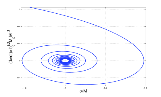
Figure 1: Typical phase curve (in the phase plane ($\phi$,$\dot{\phi})$) of the scalar field $\phi$ during the transition to $\Lambda=0$ state. For illustrative purposes the parameters are chosen such that $V_{eff}=(M^{2}/2b_{g})(\phi^{2}-M^{2})^{2}/(\phi^{2}+4M^{2})$ and $\phi_{0}=\pm M$ and $\delta=0$. In the case without fine tuning of the parameters $b_{g}\neq b_{\phi}$, i.e. $\delta\neq 0$, the phase portrait is qualitatively the same.

It follows from the constraint (102) (where we took $\delta=0$) that $|\zeta|\to\infty$ as $\phi\to\phi_{0}$. More exactly, oscillations of $sM^{4}+V_{1}$ around zero are accompanied with a singular behavior of $\zeta$ each time when $\phi$ crosses $\phi_{0}$

$$\frac{1}{\zeta}\sim sM^{4}+V_{1}(\phi)\to 0\qquad as\qquad\phi\to\phi_{0}$$ (24)

and $\zeta^{-1}$ oscillates around zero together with $sM^{4}+V_{1}(\phi)$. Taking into account that the metric in the Einstein frame $\tilde{g}_{\mu\nu}$, Eq.(23), is regular we deduce from Eq.(14) that the metric $g_{\mu\nu}$ used in the underlying action (12) becomes degenerate each time when $\phi$ crosses $\phi_{0}$

$$g_{00}=\frac{\tilde{g}_{00}}{\zeta+b_{g}}\sim\frac{1}{\zeta}\to 0;\qquad g_{ii}=\frac{\tilde{g}_{ii}}{\zeta+b_{g}}\sim-\frac{1}{\zeta}\to 0\qquad as\qquad\phi\to\phi_{0},$$ (25)

where we have taken into account that the energy density approaches zero and therefore for this cosmological solution the scale factor $a(t)$ remains finite in all times $t$. Therefore

$$\sqrt{-g}\sim\frac{1}{\zeta^{2}}\to 0\qquad and\qquad\Phi=\zeta\sqrt{-g}\sim\frac{1}{\zeta}\to 0\qquad as\qquad\phi\to\phi_{0}$$ (26)

The detailed behavior of $\zeta$, the manifold measure $\Phi$ and $g_{\mu\nu}$ - components are shown in Fig. 2.

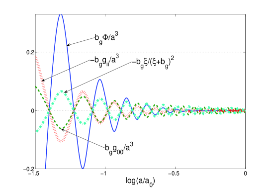
Figure 2: Oscillations of the measure $\Phi$, the original metric $g_{\mu\nu}$ and $\zeta/(\zeta+b_{g})^{2}$ during the transition to $\Lambda=0$ state.

Recall that the manifold volume measure $\Phi$ is a signed measuresigned and therefore it is not a surprise that it can change sign. But TMT shows that including the manifold degrees of freedom into the dynamics of the scalar-gravity system we discover an interesting dynamical effect: a transition to zero vacuum energy is accompanied by oscillations of $\Phi$ around zero. Similar oscillations simultaneously occur with all components of the metric $g_{\mu\nu}$ used in the underlying action (12).

The measure $\Phi$ and the metric $g_{\mu\nu}$ pass zero only in a discrete set of moments in the course of transition to the $\Lambda=0$ state. Therefore there is no problem with the condition $\Phi\neq 0$ used for the solution (6). Also there is no problem with singularity of $g^{\mu\nu}$ in the underlying action since

$$\lim_{\phi\to\phi_{0}}\Phi g^{\mu\nu}=finite\qquad and\qquad\sqrt{-g}g^{\mu\nu}\sim\frac{1}{\zeta}\to 0\qquad as\qquad\phi\to\phi_{0}$$ (27)

The metric in the Einstein frame $\tilde{g}_{\mu\nu}$ is always regular because degeneracy of $g_{\mu\nu}$ is compensated in Eq.(14) by singularity of the ratio of two measures $\zeta\equiv\Phi/\sqrt{-g}$.

In Ref.(GK9 ) we have explained in details how the presented resolution of the old CC problem avoids the well known no-go theorem by WeinbergWeinberg1 stating that generically in field theory one cannot achieve zero value of the potential in the minimum without fine tuning. It is interesting that the resolution of the old CC problem in the context of TMT happens in the regime where $\zeta\rightarrow\infty$. From the point of view of TMT, the latter is the answer to the question why the old cosmological constant problem cannot be solved (without fine tuning) in theories with only the measure of integration $\sqrt{-g}$ in the action.

V Scalar field model II. Spontaneously broken global scale invariance

V.1 Formulation of the model

Let us now turn to the analyze of the results of the TMT model possessing a global scale invariance studied early in detailG1 -GKatz ,GK5 -GK9 . The scalar field $\phi$ playing the role of a model of dark energy appears here as a dilaton, and a spontaneous breakdown of the scale symmetry results directly from the presence of the manifold volume measure $\Phi$. In other words, this SSB is an intrinsic feature of TMT.

The action of the model reads

$$S=S_{g}+S_{\phi}\quad\text{where}$$ (28)

$$S_{g} = -\frac{1}{b_{g}\kappa}\int d^{4}xe^{\alpha\phi/M_{p}}(\Phi+b_{g}\sqrt{-g})R(\Gamma,g)$$

$$S_{\phi} = \frac{1}{b_{g}}\int d^{4}xe^{\alpha\phi/M_{p}}\left[(\Phi+b_{\phi}\sqrt{-g})\frac{1}{2}g^{\mu\nu}\phi_{,\mu}\phi_{,\nu}-e^{\alpha\phi/M_{p}}\left(\Phi V_{1}+\sqrt{-g}V_{2}\right)\right]$$

and it is invariant under the global scale transformations ($\theta=const.$):

$$g_{\mu\nu}\rightarrow e^{\theta}g_{\mu\nu},\,\,\Gamma^{\mu}_{\alpha\beta}\rightarrow\Gamma^{\mu}_{\alpha\beta},\,\,\varphi_{a}\rightarrow\lambda_{ab}\varphi_{b}\,\,\text{where}\,\,\det(\lambda_{ab})=e^{2\theta},\,\,\phi\rightarrow\phi-\frac{M_{p}}{\alpha}\theta.$$ (29)

The appearance of the dimensionless parameters $b_{g}$ and $b_{\phi}$ is explained by the same reasons we mentioned after Eqs.(9) and (12). In contrast to the model of Sec.3, now we deal with exponential (pre-) potentials where $V_{1}$ and $V_{2}$ are constant dimensionfull parameters. The remarkable feature of this TMT model is that Eq.(6), being the solution of the equation of motion resulting from variation of the manifold volume measure degrees of freedom, breaks spontaneously the scale symmetry (29): this happens due to the appearance of a dimensionfull integration constant $sM^{4}$ in Eq.(6).

One can showGK9 that if $b_{g}V_{1}>V_{2}$ then the ground state appears to be again (as it was in the scalar field model I, see Secs.3 and 4) a zero CC state without fine tuning of the parameters and initial conditions in the following two cases: either $s=-1$ and $V_{1}>0$ or $s=+1$ and $V_{1}<0$. The behavior of $\Phi$ and $g_{\mu\nu}$ in the course of transition to the $\Lambda=0$ state is qualitatively the same as we observed in Sec.4.

Here, in the presentation of the results of the model (28), we restrict ourself with the choice $s=+1$ and $V_{1}<0$.

Similar to the model of Sec.3, equations of motion resulting from the action (28) are noncanonical and the space-time is non Riemannian when using the original set of variables. This is because all the equations of motion and the solution for the connection coefficients include terms proportional to $\partial_{\mu}\zeta$. However, when working with the new metric ($\phi$ remains the same)

$$\tilde{g}_{\mu\nu}=e^{\alpha\phi/M_{p}}(\zeta+b_{g})g_{\mu\nu},$$ (30)

which we call the Einstein frame, the connection becomes Riemannian and general form of all equations becomes canonical. Since $\tilde{g}_{\mu\nu}$ is invariant under the scale transformations (29), spontaneous breaking of the scale symmetry is reduced in the Einstein frame to the spontaneous breakdown of the shift symmetry

$$\phi\rightarrow\phi+const.$$ (31)

Notice that the Goldstone theorem generically is not applicable in this theoryG1 . The reason is the following. In fact, the scale symmetry (31) leads to a conserved dilatation current $j^{\mu}$. However, for example in the spatially flat FRW universe the spatial components of the current $j^{i}$ behave as $j^{i}\propto M^{4}x^{i}$ as $|x^{i}|\rightarrow\infty$. Due to this anomalous behavior at infinity, there is a flux of the current leaking to infinity, which causes the non conservation of the dilatation charge. The absence of the latter implies that one of the conditions necessary for the Goldstone theorem is missing.

After the change of variables to the Einstein frame (30) the gravitational equation takes the standard GR form with the same Newton constant as in (28)

$$G_{\mu\nu}(\tilde{g}_{\alpha\beta})=\frac{\kappa}{2}T_{\mu\nu}^{eff}$$ (32)

where $G_{\mu\nu}(\tilde{g}_{\alpha\beta})$ is the Einstein tensor in the Riemannian space-time with the metric $\tilde{g}_{\mu\nu}$. The energy-momentum tensor $T_{\mu\nu}^{eff}$ reads

$$T_{\mu\nu}^{eff} = \frac{\zeta+b_{\phi}}{\zeta+b_{g}}\left(\phi_{,\mu}\phi_{,\nu}-\frac{1}{2}\tilde{g}_{\mu\nu}\tilde{g}^{\alpha\beta}\phi_{,\alpha}\phi_{,\beta}\right)$$

$$- \tilde{g}_{\mu\nu}\frac{b_{g}-b_{\phi}}{2(\zeta+b_{g})}\tilde{g}^{\alpha\beta}\phi_{,\alpha}\phi_{,\beta}+\tilde{g}_{\mu\nu}V_{eff}(\phi,\zeta;M)$$

where the function $V_{eff}(\phi,\zeta;M)$ is defined as following:

$$V_{eff}(\phi,\zeta;M)=\frac{b_{g}\left[M^{4}e^{-2\alpha\phi/M_{p}}+V_{1}\right]-V_{2}}{(\zeta+b_{g})^{2}}.$$ (34)

The scalar field $\zeta$ is determined by means of the constraint similar to Eq.(102) of Sec.IV

$$(b_{g}-\zeta)\left[M^{4}e^{-2\alpha\phi/M_{p}}+V_{1}\right]-2V_{2}-\delta\cdot b_{g}(\zeta+b_{g})X=0$$ (35)

where

$$X\equiv\frac{1}{2}\tilde{g}^{\alpha\beta}\phi_{,\alpha}\phi_{,\beta}\qquad\text{and}\qquad\delta=\frac{b_{g}-b_{\phi}}{b_{g}}$$ (36)

The dilaton $\phi$ field equation in the Einstein frame is reduced to the following

$$\frac{1}{\sqrt{-\tilde{g}}}\partial_{\mu}\left[\frac{\zeta+b_{\phi}}{\zeta+b_{g}}\sqrt{-\tilde{g}}\tilde{g}^{\mu\nu}\partial_{\nu}\phi\right]-\frac{2\alpha\zeta}{(\zeta+b_{g})^{2}M_{p}}M^{4}e^{-2\alpha\phi/M_{p}}=0.$$ (37)

where again $\zeta$ is a solution of the constraint (35). Note that the dilaton $\phi$ dependence in all equations of motion in the Einstein frame appears only in the form $M^{4}e^{-2\alpha\phi/M_{p}}$, i.e. it results only from the spontaneous breakdown of the scale symmetry (29).

The effective energy-momentum tensor (78) can be represented in a form of that of a perfect fluid

$$T_{\mu\nu}^{eff}=(\rho+p)u_{\mu}u_{\nu}-p\tilde{g}_{\mu\nu},\qquad\text{where}\qquad u_{\mu}=\frac{\phi_{,\mu}}{(2X)^{1/2}}$$ (38)

with the following energy and pressure densities resulting from Eqs.(78) and (34) after inserting the solution $\zeta=\zeta(\phi,X;M)$ of Eq.(35):

$$\rho(\phi,X;M)=X+\frac{(M^{4}e^{-2\alpha\phi/M_{p}}+V_{1})^{2}-2\delta b_{g}(M^{4}e^{-2\alpha\phi/M_{p}}+V_{1})X-3\delta^{2}b_{g}^{2}X^{2}}{4[b_{g}(M^{4}e^{-2\alpha\phi/M_{p}}+V_{1})-V_{2}]},$$ (39)

$$p(\phi,X;M)=X-\frac{\left(M^{4}e^{-2\alpha\phi/M_{p}}+V_{1}+\delta b_{g}X\right)^{2}}{4[b_{g}(M^{4}e^{-2\alpha\phi/M_{p}}+V_{1})-V_{2}]}.$$ (40)

In a spatially flat FRW universe with the metric $\tilde{g}_{\mu\nu}=diag(1,-a^{2},-a^{2},-a^{2})$ filled with the homogeneous scalar field $\phi(t)$, the $\phi$ field equation of motion takes the form

$$Q_{1}\ddot{\phi}+3HQ_{2}\dot{\phi}-\frac{\alpha}{M_{p}}Q_{3}M^{4}e^{-2\alpha\phi/M_{p}}=0$$ (41)

where $H$ is the Hubble parameter and we have used the notations $\dot{\phi}\equiv d\phi/dt$,

$$Q_{1}=2[b_{g}(M^{4}e^{-2\alpha\phi/M_{p}}+V_{1})-V_{2}]\rho_{,X}=(b_{g}+b_{\phi})(M^{4}e^{-2\alpha\phi/M_{p}}+V_{1})-2V_{2}-3\delta^{2}b_{g}^{2}X$$ (42)

$$Q_{2}=2[b_{g}(M^{4}e^{-2\alpha\phi/M_{p}}+V_{1})-V_{2}]p_{,X}=(b_{g}+b_{\phi})(M^{4}e^{-2\alpha\phi/M_{p}}+V_{1})-2V_{2}-\delta^{2}b_{g}^{2}X$$ (43)

$$\quad Q_{3}=\frac{1}{[b_{g}(M^{4}e^{-2\alpha\phi/M_{p}}+V_{1})-V_{2}]}$$ (44)

$$\times\left[(M^{4}e^{-2\alpha\phi/M_{p}}+V_{1})[b_{g}(M^{4}e^{-2\alpha\phi/M_{p}}+V_{1})-2V_{2}]+2\delta b_{g}V_{2}X+3\delta^{2}b_{g}^{3}X^{2}\right]$$

The non-linear $X$-dependence appears here in the framework of the fundamental theory without exotic terms in the Lagrangians $L_{1}$ and $L_{2}$. This effect follows just from the fact that there are no reasons to choose the parameters $b_{g}$ and $b_{\phi}$ in the action (28) to be equal in general; on the contrary, the choice $b_{g}=b_{\phi}$ would be a fine tuning. Thus the above equations represent an explicit example of $k$-essencek-essence resulting from first principles. The system of equations (32), (39)-(41) accompanied with the functions (42)-(44) and written in the metric $\tilde{g}_{\mu\nu}=diag(1,-a^{2},-a^{2},-a^{2})$ can be obtained from the k-essence type effective action

$$S_{eff}=\int\sqrt{-\tilde{g}}d^{4}x\left[-\frac{1}{\kappa}R(\tilde{g})+p\left(\phi,X;M\right)\right],$$ (45)

where $p(\phi,X;M)$ is given by Eq.(40). In contrast to the simplified models studied in literaturek-essence , it is impossible here to represent $p\left(\phi,X;M\right)$ in a factorizable form like $\tilde{K}(\phi)\tilde{p}(X)$. The scalar field effective Lagrangian, Eq.(40), can be represented in the form

$$p\left(\phi,X;M\right)=K(\phi)X+L(\phi)X^{2}-U(\phi)$$ (46)

where the potential

$$U(\phi)=\frac{[V_{1}+M^{4}e^{-2\alpha\phi/M_{p}}]^{2}}{4[b_{g}\left(V_{1}+M^{4}e^{-2\alpha\phi/M_{p}}\right)-V_{2}]}$$ (47)

and $K(\phi)$ and $L(\phi)$ depend on $\phi$ only via $M^{4}e^{-2\alpha\phi/M_{p}}$. Notice that $U(\phi)>0$ for any $\phi$ provided

$$b_{g}>0,\qquad\text{and}\qquad b_{g}V_{1}\geq V_{2},$$ (48)

that we will assume in what follows. Note that besides the presence of the effective potential $U(\phi)$, the Lagrangian $p\left(\phi,X;M\right)$ differs from that of Ref.k-inflation-Mukhanov by the sign of $L(\phi)$: in our case $L(\phi)<0$ provided the conditions (48). This result cannot be removed by a choice of the parameters of the underlying action (28) while in Ref.k-inflation-Mukhanov the positivity of $L(\phi)$ was an essential assumption. This difference plays a crucial role for a possibility of a dynamical protection from the initial singularity of the curvature studied in detail in RefGK9 .

The model allows a power law inflation (where the dilaton $\phi$ plays the role of the inflaton) with a graceful exit to a zero or tiny cosmological constant state. In what it concerns to primordial perturbations of $\phi$ and their evolution, there are no difference with the usual (i.e. one-measure) model with the action (45)-(47).

V.2 Early power law inflation

We are going to study spatially flat FRW cosmological models governed by the system of equations

$$\frac{\dot{a}^{2}}{a^{2}}=\frac{1}{3M_{p}^{2}}\rho$$ (49)

and (39)-(41), and in this subsection we will consider the fine tuned case $\delta=0$. As $M^{4}e^{-2\alpha\phi/M_{p}}\gg Max\left(|V_{1}|,|V_{2}|/b_{g}\right)$, the effective potential (47) behaves as the exponential potential $V_{eff}^{(0)}\approx\frac{1}{4b_{g}}M^{4}e^{-2\alpha\phi/M_{p}}$. So, as $\phi\ll-M_{p}$ the model describes the well studied power law inflation of the early universepower-law if $0<\alpha<1/\sqrt{2}$ :

$$a(t)=a_{in}\left(\frac{t}{t_{in}}\right)^{1/2\alpha^{2}},\qquad\phi(t)=\frac{M_{p}}{\alpha}ln\left(\frac{\alpha^{2}M^{2}t}{M_{p}\sqrt{b_{g}(3-2\alpha^{2})}}\right).$$ (50)

In the phase plane $(\phi,\dot{\phi})$ there is only one phase curve representing these solutions and it plays the role of the attractorHalliwell for all other solutions with arbitrary initial values of $\phi_{in}$ and $\dot{\phi}_{in}$. Excluding time from $\phi(t)$ and $\dot{\phi}(t)$ we obtain the equation of the attractor in the phase plane:

$$\frac{\sqrt{b_{g}}}{M^{2}}\,\dot{\phi}=\frac{\alpha}{\sqrt{3-2\alpha^{2}}}e^{-\alpha\phi/M_{p}}.$$ (51)

With our choice of $\alpha=0.2$ the equation-of-state for the attractor is $w\approx-0.95$.

Solutions corresponding to different independent initial values $\phi_{in}$ and $\dot{\phi}_{in}$ have been studied numerically in Ref.GK9 : shapes of the phase curves are characterized by much steeper (almost vertical) approaching the attractor than the exponential shape of the decay of the attractor itself. Graceful exit from the inflationary regime was demonstrated in detail in Ref.GK9 as well.

V.3 Quintessential inflation type of scenario

The model (28) provides a possibility of a quintessential inflation type of scenarioQuint-infl where the early power law inflation ends with a graceful exit to a quintessence-like epoch. This was demonstrated in Ref.(GK9 ) in detail. Here we shortly illustrate this possibility in the case $V_{1}>0$ and $b_{g}V_{1}\geq 2V_{2}$.

In this model the effective potential (47) is a monotonically decreasing function of $\phi$. As $\phi\ll-M_{p}$ the model describes the power law inflation, similar to what we discussed in the previous subsection. Applying this model to the cosmology of the late time universe and assuming that the scalar field $\phi\rightarrow\infty$ as $t\rightarrow\infty$, it is convenient to represent the effective potential (47) in the form

$$V_{eff}^{(0)}(\phi)=\Lambda+V_{q-l}(\phi)$$ (52)

with the definition

$$\Lambda=\frac{V_{1}^{2}}{4(b_{g}V_{1}-V_{2})}.$$ (53)

Here $\Lambda$ is the positive cosmological constant (see (48)) and

$$V_{q-l}(\phi)=\frac{(b_{g}V_{1}-2V_{2})V_{1}M^{4}e^{-2\alpha\phi/M_{p}}+(b_{g}V_{1}-V_{2})M^{8}e^{-4\alpha\phi/M_{p}}}{4(b_{g}V_{1}-V_{2})[b_{g}(V_{1}+M^{4}e^{-2\alpha\phi/M_{p}})-V_{2}]},$$ (54)

that is the evolution of the late time universe is governed both by the cosmological constant $\Lambda$ and by the quintessence-like potential $V_{q-l}(\phi)$.

Thus the effective potential (47) provides a possibility for a toy cosmological scenario which passes through 3 stages: an early power law inflation, quintessence and ends with a cosmological constant $\Lambda$. Recall that the $\phi$-dependence of the effective potential (47) appears here only as the result of the spontaneous breakdown of the global scale symmetry (29) which in the Einstein frame is just a shift symmetry(31).

V.4 A tiny CC without fine tuning of dimensionfull parameters

In the scalar field models of dark energy, an interesting feature of TMT consists in a possibility to provide a small value of the cosmological constant without fine tuning of dimensionfull parameters. If in the model of the previous subsection the parameter $V_{2}<0$ and $|V_{2}|\gg b_{g}V_{1}$ then $\Lambda$ can be very small without the need for $V_{1}$ and $V_{2}$ to be very small. For example, if $V_{1}$ is determined by the energy scale of electroweak symmetry breaking $V_{1}\sim(10^{3}GeV)^{4}$ and $V_{2}$ is determined by the Planck scale $V_{2}\sim(10^{18}GeV)^{4}$ then $\Lambda\sim(10^{-3}eV)^{4}$. Along with such a seesaw mechanismG1 , seesaw , there exists another way to explain the smallness of $\Lambda$. As one can see from Eq.(53), the value of $\Lambda$ appears to be inverse proportional to the dimensionless parameter $b_{g}$ which characterizes the relative strength of the ’manifold’ and ’metrical’ parts of the gravitational action (see $S_{g}$ in (28)). If for example $V_{1}\sim(10^{3}GeV)^{4}$ then for getting $\Lambda_{1}\sim(10^{-3}eV)^{4}$ one should assume that $b_{g}\sim 10^{60}$. Such a large value of $b_{g}$ (see Eq.(9)) permits to formulate a correspondence principleGK9 between TMT and regular (i.e. one-measure) field theories: when $\zeta/b_{g}\ll 1$ then one can neglect the gravitational term in $L_{1}$ with respect to that in $L_{2}$ (see Eq.(9) or Eq.(12) or Eq.(28)). More detailed analysisGK9 ,GK11 shows that in such a case the manifold volume measure $\Phi=\zeta\sqrt{-g}$ has no a dynamical effect and TMT is reduced to GR.

VI Early TMT cosmology with no fine tuning: absence of the initial singularity of the curvature

VI.1 General analysis and numerical solutions

Let us now return to the general case of the model of Sec.5 with no fine tuning of the parameters $b_{g}$ and $b_{\phi}$, i.e. the parameter $\delta$, defined by Eq.(36), is now non zero. The dynamics of the spatially flat FRW cosmology is described by Eqs.(39)-(41) and (49). Let us start from the analysis of Eq.(41). The interesting feature of this equation is that each of the factors $Q_{i}(\phi,X)$   ($i=1,2,3$) can get to zero and this effect depends on the range of the parameter space chosen. This is the origin of drastic changes of the topology of the phase plane comparing with the fine tuned model of Sec.5.2.

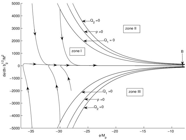
Figure 3: The phase portrait for the model with $\delta=0.1$, $\alpha=0.2$, $V_{1}=-30M^{4}$ and $V_{2}=-50b_{g}M^{4}$. All phase curves demonstrate the attractor behavior similar to that in the fine tuned case $\delta=0$, Fig.2. One can see that the attractor does not intersect the line $Q_{1}=0$, see also Fig.10. The location of the oscillatory regime marked by point $B$ is exactly the same as in the model with $\delta=0$. The essential difference consists in a novel topological structure: in the neighborhood of the line $Q_{1}=0$ all the phase curves exhibit a repulsive behavior from this line and therefore points of the line $Q_{1}=0$ are dynamically unachievable. Hence the phase curves cannot be continued infinitely to the past.

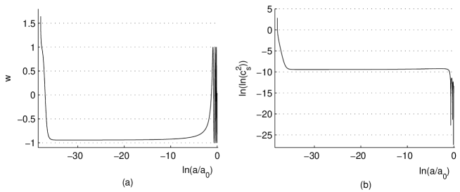
Figure 4: Typical scale factor dependence of the equation-of-state $w$ and the squared sound speed $c^{2}_{s}$ for the phase curves starting from points very close to the line $Q_{1}=0$ (in this figure - for $\phi_{in}=-30M_{p}$ and $\dot{\phi}_{in}=4540.7569b_{g}^{-1/2}M^{2}$). The squared sound speed in the starting point is $c^{2}_{s}\approx exp(exp(2.86))\approx 3.8\cdot 10^{7}$. It is not a problem to obtain more than 75 e-folds during the power law inflation (the region of $w\approx-0.95$ in Fig.(a)) just by choosing a larger absolute value $|\phi_{in}|$. We have chosen $\phi_{in}=-30M_{p}$ because this allows to show more details in these and subsequent graphs.

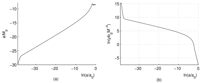
Figure 5: Typical scale factor dependence of $\phi$ and $\rho$ for the phase curves starting from points very close to the line $Q_{1}=0$ (in this figure - for the same point as in Fig.4.

For $Q_{1}\neq 0$, Eqs. (41), (49) result in the well known equationVikman

$$\ddot{\phi}+\frac{\sqrt{3\rho}}{M_{p}}c_{s}^{2}\dot{\phi}+\frac{\rho_{,\phi}}{\rho_{,X}}=0,$$ (55)

where $c_{s}$ is the effective sound speed of perturbationsGM

$$c_{s}^{2}=\frac{p_{,X}}{\rho_{,X}}=\frac{Q_{2}}{Q_{1}},$$ (56)

$$\frac{\rho_{,\phi}}{\rho_{,X}}=-\frac{\alpha}{M_{p}}\cdot\frac{Q_{3}}{Q_{1}}\cdot M^{4}e^{-2\alpha\phi/M_{p}};$$ (57)

$\rho$ and $p$ are defined by Eqs.(39), (40) and $Q_{i}$ $(i=1,2,3)$ - by Eqs.(42)-(44).

It follows from the definitions of $Q_{1}$ and $Q_{2}$ that $c_{s}^{2}>1$ when $Q_{1}>0$ and $X>0$ (that implies $Q_{2}>0$). Therefore in the cosmological FRW background, the sound speed of perturbations can be bigger than speed of lightBabichev-Mukh .

In the model with $V_{1}<0$ and $V_{2}<0$, the structure of the phase plane is presented in Fig.3. With a choice of the parameters made, the following condition is satisfied

$$(b_{g}+b_{\phi})V_{1}-2V_{2}>0.$$ (58)

As we will see in Sec.7, the latter is the characteristic condition which determines the structure of the phase plane. By the two branches of the line $Q_{1}=0$, the phase plane is divided into three large dynamically disconnected zones. In the most part of two of them (II and III), the energy density is negative ($\rho<0$). In the couple of regions between the lines $Q_{1}=0$ and $\rho=0$ that we refer for short as ($Q_{1}\rightarrow\rho$)-regions, $\rho>0$ but $Q_{1}<0$. Typical scale factor dependence of the equation-of-state $w$, the sound speed of perturbations $c_{s}^{2}$, the inflaton $\phi$ and the energy density $\rho$ are presented in Figs.4 and 5. It is not a problem to obtain more than 75 e-folds during the power law inflation (the region of $w\approx-0.95$ in Fig.4a) just by choosing a larger absolute value $|\phi_{in}|$. We have chosen $\phi_{in}=-30M_{p}$ because this allows to show more details in these graphs.

The zone I of the phase plane (where $Q_{1}>0$, $\rho>0$ and $Q_{2}>0$) is of a great cosmological interest:

a)   Similar to what we have seen in the fine tuned case in Sec.5.2, all the phase curves start with very steep approach to an attractor. The nonlinearity in $X$ does not allow to obtain an exact analytic solution in the model under consideration and therefore we have no here the analytic equation of the attractor. But one can showGK9 that, with our choice of the parameters $\alpha$ and $\delta$, the emergence of the additional terms $\propto\delta X$ and $\propto\delta^{2}X^{2}$ in the model under consideration results in small enough corrections to the equation of the attractor in comparison with Eq.(51) of the fined tuned model of Sec.IVB. For our qualitative analysis below one can use Eq.(51) as a good approximation to the true attractor equation.

b)   Comparing the equation of the line $Q_{1}=0$, which for $\phi\ll-M_{p}$ can be written in the form

$$\frac{\sqrt{b_{g}}}{M^{2}}\,\dot{\phi}=\pm\frac{1}{\delta}\sqrt{\frac{2}{3}(2-\delta)}\cdot e^{-\alpha\phi/M_{p}}+O\left(\frac{V_{1}}{M^{4}}e^{\alpha\phi/M_{p}}\right),$$ (59)

with the equation of the attractor which approximately coincides with Eq.(51), we see that the upper brunch of the line $Q_{1}=0$ has actually the same form of a decaying exponent as the attractor, but the factor in front of the exponent in Eq.(59) is about $10^{2}$ times bigger than in Eq.(51). The above analytic estimations are confirmed by the numerical solutions as one can see in Fig.3. This means that the attractor does not intersect the line $Q_{1}=0$. Therefore all the phase curves starting in zone I arrive at the attractor (of course asymptotically).

c)   In the neighborhood of the line $Q_{1}=0$ all the phase curves exhibit a repulsive behavior from this line. In other words, the shape of two branches of $Q_{1}=0$ do not allow a classical dynamical continuation of the phase curves backward in time without crossing the classical barrier formed by the line $Q_{1}=0$. This is true for all finite values of the initial conditions $\phi_{in}$, $\dot{\phi}_{in}$ in zone I.

d)  As one can see from Fig.4a, the initial stage of evolution is very much different from the subsequent one, that is a power law inflation. This fact may have a relation to the results of the study of completeness of inflationary cosmological models in past directionsBGV .

e)  If the phase curves start from points $(\phi_{in},\dot{\phi}_{in})$ in zone I very close to the line $Q_{1}=0$ then the sound speed of perturbations has huge values at the beginning of the evolution, see Figs.4b. However in the power law inflation stage, $c_{s}$ is too close to the speed of light and appears to be unable to increase the tensor-to-scalar perturbation ratioGM .

In two regions between the lines $Q_{1}=0$ and $Q_{2}=0$ that we refer for short as ($Q_{1}\rightarrow Q_{2}$)-regions,, the squared sound speed of perturbations is negative, $c_{s}^{2}<0$. This means that on the right hand side of the classical barrier $Q_{1}=0$, the model is absolutely unstable. Moreover, this pure imaginary sound speed becomes infinite in the limit $Q_{1}\rightarrow 0-$. Thus the branches of the line $Q_{1}=0$ divide zone I (of the classical dynamics) from the ($Q_{1}\rightarrow Q_{2}$)-regions where the physical significance of the model is unclear. Note that the line $\rho=0$ divides the ($Q_{1}\rightarrow Q_{2}$)-regions into two subregions with opposite signs of the classical energy density.

Thus the structure of the phase plane yields a conclusion that the starting point of the classical history in the phase plane can be only in zone I and the line $Q_{1}=0$ is the limiting set of points where the classical history might begin. For any finite initial values of $\phi_{in}$ and $\dot{\phi}_{in}$ at the initial cosmic time $t_{in}$, the duration $t_{in}-t_{s}$ of the continuation of the evolution into the past up to the moment $t_{s}$ when the phase trajectory arrives the line $Q_{1}=0$, is finite.

VI.2 Analysis of the initial singularity

Let us analyze what happens as $t\to t_{s}$ (and $Q_{1}(\phi,\dot{\phi})\to 0$) if this continuation to the past starts from a point in zone I of the phase plane with finite initial values $\phi_{in}$ and $\dot{\phi}_{in}$ . First note that the energy density $\rho_{s}=\rho(t_{s})$ and the pressure $p_{s}=p(t_{s})$ are finite in all the points of the line $Q_{1}=0$ with finite coordinates $\phi_{s}=\phi(t_{s})$, $\dot{\phi_{s}}=\dot{\phi}(t_{s})$, that it is easy to see from Eqs.(39), (40) and (42). The strong energy condition is satisfied in regions of zone I close to the line $Q_{1}=0$ including the line itself. In fact, for any unit time-like vector $t^{\mu}$ we have on the line $Q_{1}=0$

$$\left(T_{\mu\nu}^{eff}-\frac{1}{2}\tilde{g}_{\mu\nu}T^{eff}\right)t^{\mu}t^{\nu}=\frac{1}{2}(\rho_{s}+3p_{s})\approx\frac{2b_{\phi}}{(b_{g}-b_{\phi})^{2}}M^{4}e^{-2\alpha\phi_{s}/M_{p}}>0,$$ (60)

where $T_{\mu\nu}^{eff}$ is defined in Eq.(38), $T^{eff}\equiv\tilde{g}^{\mu\nu}T_{\mu\nu}^{eff}$ and we have taken into account our choice of the parameters ($b_{g}>0$, $b_{\phi}>0$ and Eq.(48)) and assumed that $M^{4}e^{-2\alpha\phi_{s}/M_{p}}\gg|V_{1}|$. This result is in the total agreement with the numerical solutions of the previous subsection. In particular, the described analytic approximation on the line $Q_{1}=0$ yields $w_{s}=p_{s}/\rho_{s}\approx 5/3$ which is in a very good agreement with the numerical results obtained in regions of zone I close enough to the line $Q_{1}=0$, see Fig.4a.

It follows from the Einstein equations (49) and

$$\frac{\ddot{a}}{a}=-\frac{1}{6M_{p}^{2}}(\rho+3p)$$ (61)

that the first and second time derivatives of the scale factor, $\dot{a}_{s}=\dot{a}(t_{s})$ and $\ddot{a}_{s}=\ddot{a}(t_{s})$, and therefore the curvature, are finite on the line $Q_{1}=0$. The time derivative of the energy density also approaches a finite value

$$\dot{\rho}_{s}=3\frac{\dot{a}_{s}}{a_{s}}(\rho_{s}+p_{s})<\infty$$ (62)

but $\dot{p}\to-\infty$   as   $t\to t_{s}$ because $|\ddot{\phi}|\to\infty$.

The detailed analysis shows that

$$a(t)\approx a_{s}+A(t-t_{s})^{5/2}\quad\text{and}\quad\dot{\phi}=\dot{\phi}_{s}\pm\frac{M_{p}}{2\alpha}\sqrt{2B(t-t_{s})}\quad\text{as}\quad t\to t_{s},$$ (63)

where $A>0$ and $B>0$i are constants in time.

Therefore although the scalar curvature

$$R=-6(\frac{\ddot{a}}{a}+\frac{\dot{a}^{2}}{a^{2}})$$ (64)

is finite as $t\to t_{s}$ but its time derivative is singular:

$$\dot{R}\approx-6\frac{\dddot{a}}{a}\to-\infty\qquad\text{as}\qquad t\to t_{s}$$ (65)

This type of singularity we discover here in the framework of the dynamical model is present in the classification of ”sudden” singularities given by BarrowBarrow1 .

Finally we want to discuss possible scales of the energy when the initial conditions are close to the line $Q_{1}=0$. If $\phi_{in}\approx\phi_{s}\ll-M_{p}$ then approximately

$$\rho_{in}\approx\rho_{s}\approx\frac{(b_{g}+b_{\phi})^{2}}{12b_{g}(b_{g}-b_{\phi})^{2}}M^{4}e^{-2\alpha\phi_{s}/M_{p}}$$ (66)

Therefore depending on the parameters and initial conditions, the described mild singular initial behavior is possible for the energy densities close to the Planck scale as well as for the energy densities much lower the quantum Planck era. It is interesting that the singularity of the time derivative of the curvature on the line $Q_{1}=0$ is accompanied with singularity of the sound speed of perturbations $c_{s}^{2}=Q_{2}/Q_{1}\sim\ddot{\phi}\sim(t-t_{s})^{-1/2}$. Therefore generation of any mode of scalar fluctuations in states extremely close to the line $Q_{1}=0$ requires extremely large energy. Thus the initial state formed in the close neighborhood of the line $Q_{1}=0$ must be practically the ground state. This allows to hope that the effect $c_{s}^{2}\to\infty$ could help to solve the problem of the initial conditions in inflationary cosmology.

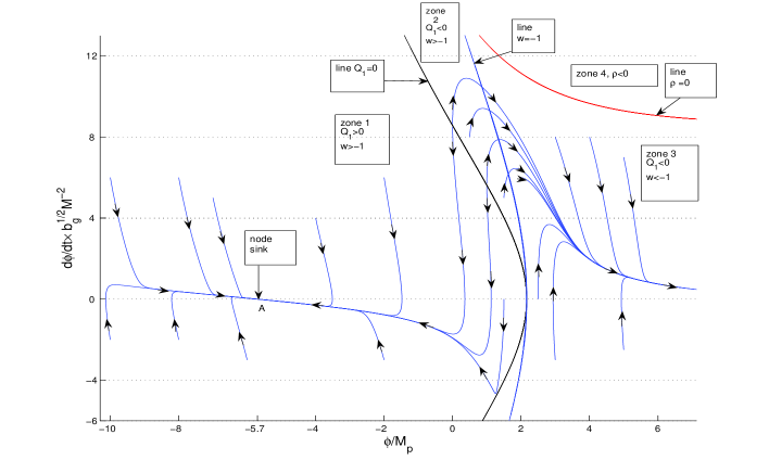
Figure 6: The phase portrait (in the phase plane ($\phi$,$\dot{\phi})$) for the model with $\alpha=0.2$, $\delta=0.1$, $V_{1}=10M^{4}$ and $V_{2}=9.9b_{g}M^{4}$. The region with $\rho>0$ is divided into two dynamically disconnected regions by the line $Q_{1}(\phi,\dot{\phi})=0$. To the left of this line $Q_{1}>0$ (the appropriate zone we call zone 1) and to the right   $Q_{1}<0$. The $\rho>0$ region to the right of the line $Q_{1}(\phi,\dot{\phi})=0$ is divided into two zones (zone 2 and zone 3) by the line $Q_{2}=0$ (the latter coincides with the line where $w=-1$). In zone 2   $w>-1$ but $c_{s}^{2}<0$. In zone 3  $w<-1$ and $c_{s}^{2}>0$. Phase curves started in zone 2 cross the line $w=-1$. All phase curves in zone 3 exhibit processes with super-accelerating expansion of the universe. Besides all the phase curves in zone 3 demonstrate attractor behavior to the line which asymptotically, as $\phi\to\infty$, approaches the straight line $\dot{\phi}=0$.

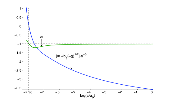
Figure 7: For the same model as in Fig. 6 and with the initial conditions $\phi_{in}=M_{p}$, $\dot{\phi}_{in}=5.7M^{2}/\sqrt{b_{g}}$: crossing the phantom divide $w=-1$ and changing sign of the total volume measure $(\Phi+b_{\phi}\sqrt{-g})$ in the scalar field $\phi$ kinetic term (in the underlying action (28)) occur simultaneously.

VII Sign indefiniteness of the manifold volume measure as the origin of a phantom dark energy

We turn now to the non fine-tuned case of the model of Sec.VII applied to the spatially flat universe. We start from a short review of our recent resultsGK9 concerning qualitative structure of the appropriate dynamical system which consists of Eqs. (41), (49) where the energy density $\rho$ is defined by Eq.(39). The case of the interest of this section is realized when the parameters of the model satisfy the condition

$$(b_{g}+b_{\phi})V_{1}-2V_{2}<0$$ (67)

In this case the phase plane has a very interesting structure presented in Fig.6. Recall that the functions $Q_{1}$, $Q_{2}$, $Q_{3}$ are defined by Eqs.(42)-(44).

We are interested in the equation of state $w=p/\rho<-1$, where pressure $p$ and energy density $\rho$ are given by Eqs.(39) and (40). The line indicated in Fig. 6 as ”line $w=-1$” coincides with the line $Q_{2}(\phi,X)=0$ because

$$w+1=\frac{X}{\rho}\cdot\frac{Q_{2}}{\left[b_{g}\left(M^{4}e^{-2\alpha\phi/M_{p}}+V_{1}\right)-V_{2}\right]}$$ (68)

Phase curves in zone 3 correspond to the cosmological solutions with the equation of state $w<-1$. In zone 2, $w>-1$ but this zone has no physical meaning since the squared sound speed of perturbations

$$c_{s}^{2}=\frac{Q_{2}}{Q_{1}}$$ (69)

is negative in zone 3. But in zone 2, $c_{s}^{2}>0$. Some details of numerical solutions describing the cross of the phantom divide $w=-1$ are presented in Fig. 7.

Note that the superaccelerating cosmological expansion is obtained here without introducing an explicit phantom scalar field into the underlying action (28). In Ref.GK9 we have discussed this effect from the point of view of the effective k-essence model realized in the Einstein frame when starting from the action (28). A deeper analysisGK11 of the same effect yields the conclusion that the true and profound origin of the appearance of an effective phantom dynamics in our model is sign-indefiniteness of the manifold volume measure $\Phi$. In fact, using the constraint (35), Eqs.(68) and (30) it is easy to show that

$$\Phi+b_{\phi}\sqrt{-g}=(w+1)\,\frac{\rho}{4X}\,\frac{[M^{4}e^{-2\alpha\phi/M_{p}}+V_{1}+\delta\cdot b_{g}X]}{[b_{g}(M^{4}e^{-2\alpha\phi/M_{p}}+V_{1})-V_{2}]}\,a^{3},$$ (70)

where $a$ is the scale factor. The expression in the l.h.s of this equation is the total volume measure of the $\phi$ kinetic term in the underlying action (28):

$$\int d^{4}x(\Phi+b_{\phi}\sqrt{-g})\frac{1}{2}g^{\mu\nu}\phi_{,\mu}\phi_{,\nu}$$ (71)

The sign of this volume measure coincides with the sign of $w+1$ as well as with the sign of the function $Q_{2}$ (see Eq.(68)). In Fig. 8 we present the result of numerical solution for the scale factor dependence of $w$ and $(\Phi+b_{\phi}\sqrt{-g})/a^{3}$. Thus crossing the phantom divide occurs when the total volume measure of the $\phi$ kinetic term in the underlying action changes sign from positive to negative for dynamical reasons. This dynamical effect appears here as a dynamically well-founded alternative to the usually postulated phantom kinetic term of a scalar field LagrangianPhantom-usual .

VIII Including fermions into the model II

VIII.1 Description of the model

The scale invariant TMT model of Sec.5 allows a generalization by involving fermions as well as gauge and Higgs fields in such a way that the standard particle model can be obtained. In this short review, to simplify the presentation of the main results we will study an Abelian gauge model which does not include the Higgs fields and quarks and chiral properties of fermions are ignored. In this simplified model the mass terms for Dirac spinors are included by hand from the very beginning into the Lagrangians $L_{1}$ and $L_{2}$. The matter content of our model includes the dilaton scalar field $\phi$, two so-called primordial fermion fields (the primordial neutrino $N$ and the primordial electron $E$) and electromagnetic field $A_{\mu}$. The latter is included in order to display the reasons why the gauge fields dynamics is canonical. Generalization to non-Abelian gauge models including also quarks, Higgs fields, the Higgs mechanism of mass generation and taking into account chiral properties of fermions is straightforward, see Ref.GK5 .

We allow in both $L_{1}$ and $L_{2}$ all the usual terms considered in standard field theory models in curved space-time. It is convenient to represent the action in the following form:

$$S=S_{g}+S_{\phi}+S_{f}+S_{em}\quad\text{where}$$ (72)

$$S_{f}=\int d^{4}xe^{\alpha\phi/M_{p}}(\Phi+k\sqrt{-g})\frac{i}{2}\sum_{i}\overline{\Psi}_{i}\left(\gamma^{a}e_{a}^{\mu}\overrightarrow{\nabla}^{(i)}_{\mu}-\overleftarrow{\nabla}^{(i)}_{\mu}\gamma^{a}e_{a}^{\mu}\right)\Psi_{i}$$ (73)

$$-\int d^{4}xe^{\frac{3}{2}\alpha\phi/M_{p}}\left[(\Phi+h_{E}\sqrt{-g})\mu_{E}\overline{E}E+(\Phi+h_{N}\sqrt{-g})\mu_{N}\overline{N}N\right]$$

$$S_{em}=-\frac{1}{4}\int d^{4}x\sqrt{-g}g^{\alpha\beta}g^{\mu\nu}F_{\alpha\mu}F_{\beta\nu}$$ (74)

and $S_{g}$, $S_{\phi}$ are determined in Eq.(28) where we take for simplicity $b_{g}=b_{\phi}=b$.   $\Psi_{i}$ ($i=N,E$) is the general notation for the primordial fermion fields $N$ and $E$; $F_{\alpha\beta}=\partial_{\alpha}A_{\beta}-\partial_{\beta}A_{\alpha}$; $\mu_{N}$ and $\mu_{E}$ are the mass parameters; $\overrightarrow{\nabla}^{(N)}_{\mu}=\vec{\partial}+\frac{1}{2}\omega_{\mu}^{cd}\sigma_{cd}$, $\overrightarrow{\nabla}^{(E)}_{\mu}=\vec{\partial}+\frac{1}{2}\omega_{\mu}^{cd}\sigma_{cd}+ieA_{\mu}$; $R(\omega,V)=e^{a\mu}e^{b\nu}R_{\mu\nu ab}(\omega)$ is the scalar curvature; $e_{a}^{\mu}$ and $\omega_{\mu}^{ab}$ are the vierbein and spin-connection; $g^{\mu\nu}=e^{\mu}_{a}e^{\nu}_{b}\eta^{ab}$ and $R_{\mu\nu ab}(\omega)=\partial_{mu}\omega_{\nu ab}+\omega^{c}_{\mu a}\omega_{\nu cb}-(\mu\leftrightarrow\nu)$. If Higgs field were included into the model then $V_{1}$ and $V_{2}$ would turn into functions of the Higgs field. Constants $b,k,h_{N},h_{E}$ are non specified dimensionless real parameters and we will only assume that they have close orders of magnitude

$$b\sim k\sim h_{N}\sim h_{E}.$$ (75)

The action (72) is evidently gauge invariant and besides it is invariant under the global scale transformations:

$$e_{\mu}^{a}\rightarrow e^{\theta/2}e_{\mu}^{a},\quad\omega^{\mu}_{ab}\rightarrow\omega^{\mu}_{ab},\quad\varphi_{a}\rightarrow\lambda_{ab}\varphi_{b}\quad A_{\alpha}\rightarrow A_{\alpha},$$

$$\phi\rightarrow\phi-\frac{M_{p}}{\alpha}\theta,\quad\Psi_{i}\rightarrow e^{-\theta/4}\Psi_{i},\quad\overline{\Psi}_{i}\rightarrow e^{-\theta/4}\overline{\Psi}_{i},$$ (76)

$$\text{where}\quad\theta=\text{const},\quad\lambda_{ab}=\text{const}\quad and\quad\det(\lambda_{ab})=e^{2\theta},$$

We have chosen the kinetic term of $A_{\mu}$ in the conformal invariant form which is possible if it is coupled only to the measure $\sqrt{-g}$. Introducing the coupling of this term to the measure $\Phi$ would lead to the nonlinear field strength dependence in the $A_{\mu}$ equation of motion. One of the possible consequences of this may be non positivity of the energy density. Another consequence is a possibility of certain unorthodox effects, like space-time variations of the effective fine structure constant. This subject deserves a special study but it is out of the purposes of this paper where the model is studied setting $F_{\mu\nu}\equiv 0$ in the solutions.

Variation of the measure fields $\varphi_{a}$ yields Eq.(6) where $L_{1}$ is defined as the part of the integrand of the action (72)-(74) coupled to the measure $\Phi$. The appearance of the integration constant $sM^{4}$ in Eq.(6) spontaneously breaks the global scale invariance (76). In what follows we choose $s=+1$.

Except for the $A_{\mu}$ equation, all other equations of motion resulting from (72)-(74) in the first order formalism contain terms proportional to $\partial_{\mu}\zeta$ that makes the space-time non-Riemannian and equations of motion - non canonical. However, with the new set of variables ($\phi$ and $A_{\mu}$ remain unchanged)

$$\tilde{e}_{a\mu}=e^{\frac{1}{2}\alpha\phi/M_{p}}(\zeta+b)^{1/2}e_{a\mu},\quad\tilde{g}_{\mu\nu}=e^{\alpha\phi/M_{p}}(\zeta+b)g_{\mu\nu},$$

$$\Psi^{\prime}_{i}=e^{-\frac{1}{4}\alpha\phi/M_{p}}\frac{(\zeta+k)^{1/2}}{(\zeta+b)^{3/4}}\Psi_{i},\quad i=N,E$$ (77)

which we call the Einstein frame, the spin-connections become those of the Einstein-Cartan space-time. Since $\tilde{e}_{a\mu}$, $\tilde{g}_{\mu\nu}$, $N^{\prime}$ and $E^{\prime}$ are invariant under the scale transformations (76), spontaneous breaking of the scale symmetry is reduced in the new variables to the spontaneous breaking of the shift symmetry (31).

After the change of variables (77) to the Einstein frame and some simple algebra, the gravitational equations take the standard GR form (32) where the energy-momentum tensor $T_{\mu\nu}^{eff}$ is now

$$T_{\mu\nu}^{eff} = \phi_{,\mu}\phi_{,\nu}-\frac{1}{2}\tilde{g}_{\mu\nu}\tilde{g}^{\alpha\beta}\phi_{,\alpha}\phi_{,\beta}+\tilde{g}_{\mu\nu}V_{eff}(\phi,\zeta;M)$$ (78)

$$+ T_{\mu\nu}^{(em)}+T_{\mu\nu}^{(ferm,can)}+T_{\mu\nu}^{(ferm,noncan)},$$

where $V_{eff}(\phi,\zeta;M)$ is defined by Eq.(34),   $T_{\mu\nu}^{(em)}$ is the canonical energy momentum tensor of the electromagnetic field; $T_{\mu\nu}^{(ferm,can)}$ is the canonical energy momentum tensor for (primordial) fermions $N^{\prime}$ and $E^{\prime}$ in curved space-time (including also interaction of $E^{\prime}$ with $A_{\mu}$). $T_{\mu\nu}^{(ferm,noncan)}$ is the noncanonical contribution of the fermions into the energy momentum tensor

$$T_{\mu\nu}^{(ferm,noncan)}=-\tilde{g}_{\mu\nu}\Lambda_{dyn}^{(ferm)}$$ (79)

where

$$\Lambda_{dyn}^{(ferm)}\equiv Z_{N}(\zeta)m_{N}(\zeta)\overline{N^{\prime}}N^{\prime}+Z_{E}(\zeta)m_{E}(\zeta)\overline{E^{\prime}}E^{\prime}$$ (80)

and the function $Z_{i}(\zeta)$ and fermion masses $m_{i}(\zeta)$ ($i=N^{\prime},E^{\prime}$) are respectively

$$Z_{i}(\zeta)\equiv\frac{(\zeta-\zeta^{(i)}_{1})(\zeta-\zeta^{(i)}_{2})}{2(\zeta+k)(\zeta+h_{i})},\qquad m_{i}(\zeta)=\frac{\mu_{i}(\zeta+h_{i})}{(\zeta+k)(\zeta+b)^{1/2}}$$ (81)

where

$$\zeta_{1,2}^{(i)}=\frac{1}{2}\left[k-3h_{i}\pm\sqrt{(k-3h_{i})^{2}+8b(k-h_{i})-4kh_{i}}\,\right].$$ (82)

The noncanonical contribution $T_{\mu\nu}^{(ferm,noncan)}$ of the fermions into the energy momentum tensor has the transformation properties of a cosmological constant term but it is proportional to fermion densities $\overline{\Psi}^{\prime}_{i}\Psi^{\prime}_{i}$   ($i=N^{\prime},E^{\prime}$).

The ”dilaton” $\phi$ field equation in the Einstein frame reads

$$\Box\phi-\frac{\alpha}{M_{p}(\zeta+b)}\left[M^{4}e^{-2\alpha\phi/M_{p}}-\frac{(\zeta-b)V_{1}(\upsilon)+2V_{2}(\upsilon)}{\zeta+b}\right]=-\frac{\alpha}{M_{p}}\Lambda_{dyn}^{(ferm)},$$ (83)

where $\Box\phi=(-\tilde{g})^{-1/2}\partial_{\mu}(\sqrt{-\tilde{g}}\tilde{g}^{\mu\nu}\partial_{\nu}\phi)$.

One can show that equations for the primordial fermions in terms of the variables (77) take the standard form of fermionic equations for $N^{\prime}$ and $E^{\prime}$ in the Einstein-Cartan space-time where the standard electromagnetic interaction of $E^{\prime}$ is present too. Besides fermion $4$-currents have the canonical form and are covariantly conserved. In what it concerns the fermion equations, all the novelty as compared with the standard field theory approach consists of the form of the $\zeta$ depending ”masses” of the primordial fermions, second equation in Eq.(81).

The electromagnetic field equations are canonical due to our choice for the appropriate term in the action (74) to be conformally invariant.

The scalar field $\zeta\equiv\Phi/\sqrt{-g}$ is determined as a function of the scalar field $\phi$ and $\overline{\Psi}^{\prime}_{i}\Psi^{\prime}_{i}$   ($i=N^{\prime},E^{\prime}$) by the following constraint

$$\frac{1}{(\zeta+b)^{2}}\left\{(b-\zeta)\left[M^{4}e^{-2\alpha\phi/M_{p}}+V_{1}(\upsilon)\right]-2V_{2}(\upsilon)\right\}=\Lambda_{dyn}^{(ferm)}$$ (84)

which is a straightforward generalization of the constraint (35) in the presence of fermions (recall that we have chosen here $\delta=0$).

One should point out an unexpected and very important fact, namely that the same function $\Lambda_{dyn}^{(ferm)}$, Eq.(80), emerges in three different places:  a) in the form of the noncanonical fermion contribution to the energy-momentum tensor, Eq.(79);  b) in the effective Yukawa coupling of the dilaton $\phi$ to fermions (see the right hand side of Eq.(83));  c) as the right hand side of the constraint.

Note that the original action (72)-(74) contains exponents of the scalar field $\phi$ and in particular the coupling of fermions with $\phi$ is realized in (72)-(74) only through the exponents of $\phi$. Nevertheless, except for the term $M^{4}e^{-2\alpha\phi/M_{p}}$ originated by the scale symmetry breaking, the equations of motion in the Einstein frame do not contain explicitly the exponents of $\phi$ . However, the Yukawa-type coupling of the fermions to $\phi$ emerges in the Einstein frame, see the r.h.s. of Eq.(83). It is interesting that non-explicit dependence on the exponent of $\phi$ in the equations of motion is actually present after solving the constraint (84) for $\zeta$. However this dependence is again in the form of $M^{4}e^{-2\alpha\phi/M_{p}}$. Thus the exponential $\phi$-dependence in the equations of motion results only from the scale symmetry breaking. Recall that in the Einstein frame the scale symmetry transformations (76) are reduced to the shift symmetry $\phi\rightarrow\phi+const$.

VIII.2 Fermionic matter in normal conditions: reproducing GR and fine tuning free decoupling from the quintessence field

VIII.2.1 Meaning of the constraint, regular fermions and reproducing Einstein equations

The detailed analysis showsGK5 ,GK7 that the l.h.s. of the constraint (84) has the order of magnitude close to that of the (quintessence) dark energy density. At the same time, in the presence of a single massive primordial fermion, the r.h.s. of the constraint (84) contains factor $m_{i}(\zeta)\overline{\Psi}^{\prime}_{i}\Psi^{\prime}_{i}$,   which have typical order of magnitude of the fermion canonical energy density $T_{00}^{(ferm,can)}$. In other words, the constraint describes the local balance between the fermion energy density and the scalar dark energy density in the space-time region where the wave function of the primordial fermion is not equal to zero; this balance is realized due to the factor $Z_{i}(\zeta)$. By means of this balance the constraint determines the scalar $\zeta(x)$ which appears to be generically a function of $\overline{\Psi}^{\prime}_{i}\Psi^{\prime}_{i}$.

Existence of a noncanonical contribution to the energy-momentum tensor (79), along with the $\zeta$ dependence of the fermion mass (second equation in (81)) means that generically primordial fermions are very much different from the regular fermions in the appropriate field theory model (with the only volume measure $\sqrt{-g}$). It is however evident that in normal particle physics conditions, that is when the energy density of a single fermion is tens of orders of magnitude larger than the vacuum energy density, the balance dictated by the constraint is satisfied in the present day universe only if

$$Z_{i}(\zeta)\approx 0\quad\Longrightarrow\quad\zeta=\zeta_{1}^{i}\quad or\quad\zeta=\zeta_{2}^{i},\quad i=N^{\prime},E^{\prime}.$$ (85)

with an extraordinarily high accuracy. Then the fermion mass (81) becomes constant and the noncanonical contribution of the fermion into the energy-momentum tensor, Eq.(79), becomes utterly negligible in comparison with the canonical contribution of the fermion into the energy-momentum tensor. Thus, if massive fermions are in normal particle physics conditions, they are described by the standard field theory equations with constant fermion mass, and, under the same conditions, gravitational equations (32) with the energy-momentum tensor determined by Eqs.(78)-(82) are reduced to the Einstein equations in the appropriate field theory model (i.e. when the scalar field, electromagnetic field and massive fermions are sources of gravity). Taking into account the undisputed fact that the classical tests of GR deal only with fermionic matter in normal particle physics conditions we conclude that although TMT belongs to alternative gravitational theories, it provides quite standard picture which includes GR and regular particle physics in all cases when the fermion energy density is tens of orders of magnitude larger than the vacuum energy density. One can suggest two alternative approaches to the question of how a primordial fermion can be realized as a regular one (see details in Sec.6.2 of Ref.GK7 ).

VIII.2.2 Resolution of the 5-th force problem for regular fermions

Reproducing Einstein equations when the primordial fermions are in the states of the regular fermions is not enough in order to assert that GR is reproduced. The reason is that at the late universe, as $\phi\gg M_{p}$, the scalar field $\phi$ effective potential is very flat and therefore due to the Yukawa-type coupling of massive fermions to $\phi$, (the r.h.s. of Eq.(83)), the long range scalar force appears to be possible in general. The Yukawa coupling ”constant” is $\alpha\frac{m_{i}(\zeta)}{M_{p}}Z_{i}(\zeta)$. Applying our analysis of the meaning of the constraint, it is easy to see that for regular fermions with $\zeta^{(i)}=\zeta_{1,2}^{(i)}$ the factor $Z_{i}(\zeta)$ is of the order of the ratio of the vacuum energy density to the regular fermion energy density. Thus we conclude that the 5-th force is extremely suppressed for the fermionic matter observable in classical tests of GR. It is very important that this result is obtained automatically, without tuning of the parameters and it takes place for both approaches to realization of the regular fermions in TMT.

VIII.3 Nonrelativistic neutrinos and dark energy

It turns out that besides the normal particle physics situations, TMT predicts possibility of so called neutrino dark energyNelson . Roughly speaking such exotic state may be created in TMT if the degree of localization of the fermion is very small. A possible way to get up such a state might be spreading of the wave packet of non-relativistic neutrino lasting a very long (of the cosmological scale) time.

We have studied in detail a modelGK7 where the spatially flat FRW universe filled with the homogeneous scalar field $\phi$ and a cold gas of uniformly distributed non-relativistic neutrinos. Then the constraint (84) takes the form

$$\frac{(b-\zeta)\left[M^{4}e^{-2\alpha\phi/M_{p}}+V_{1}\right]-2V_{2}}{(\zeta+b)^{3/2}}=\frac{(\zeta-\zeta^{(N)}_{1})(\zeta-\zeta^{(N)}_{2})}{(\zeta+k)^{2}}\mu_{N}\frac{const}{a^{3}},$$ (86)

where we have used that $\overline{N}^{\prime}N^{\prime}=\frac{const}{a^{3}}$ and $a=a(t)$ is the scale factor.

There is a solution where the decaying fermion contribution to the constraint $\sim\frac{const}{a^{3}}$ is accompanied by approaching $\zeta\rightarrow-k$ in such a way that $(\zeta+k)^{-2}\propto a^{3}$. Then both the r.h.s. and the l.h.s. of the constraint (86) approach a constant if $\phi\rightarrow\infty$ as $a(t)\rightarrow\infty$. The effective mass of the neutrino in this state increases like $(\zeta+k)^{-1}\propto a^{3/2}$ and therefore $\rho_{(N,canon)}=T_{00}^{(N,canon)}=m_{N}(\zeta)\overline{N}^{\prime}N^{\prime}\propto a^{-3/2}$. At the same time $\Lambda_{dyn}^{(N)}\propto(\zeta+k)^{-2}\overline{N}^{\prime}N^{\prime}\rightarrow constant$. This means that at the late time universe, the canonical neutrino energy density $\rho_{(N,canon)}$ becomes negligible in comparison with the non-canonical neutrino energy density $\rho_{(N,noncanon)}=T_{00}^{(N,noncanon)}=-\Lambda_{dyn}^{(N)}$. It follows then from Eq.(79) that such cold neutrino matter possesses a pressure $p_{N}$ and its equation of state in the late time universe approaches the form $p_{N}=-\rho_{N}$ typical for a cosmological constant. Therefore the primordial non-relativistic neutrino in the described regime behaves as a sort of dark energy and contributions of the quintessence-like field $\phi$ and the primordial neutrino into the dark energy density are of the same order of magnitude. We refer to this regime as Cosmo-Low-Energy-Physics (CLEP) state. The surprise is that such a CLEP state is energetically more preferableGK7 than the one in the absence of fermions case.

For a particular value of the parameter $\alpha=\sqrt{3/8}$. the cosmological equations allow the following analytic solutionGK7 for the late time universe in the CLEP regime:

$$\phi(t)=\text{const.}+\frac{M_{p}}{2\alpha}\ln(M_{p}t),\qquad a(t)\propto t^{1/3}e^{\lambda t},$$ (87)

where

$$\lambda=\frac{1}{M_{p}}\sqrt{\frac{\Lambda}{3}},\qquad\Lambda=\frac{V_{2}-kV_{1}}{(b-k)^{2}}.$$ (88)

The mass of the neutrino in such CLEP state increases exponentially in time and its $\phi$ dependence is double-exponential:

$$m_{N}|_{clep}\sim(\zeta+k)^{-1}\sim a^{3/2}(t)\sim t^{1/2}e^{\frac{3}{2}\lambda t}\sim\exp\left[\frac{3\lambda e^{-\varphi_{0}}}{2M_{p}}\exp\left(\frac{2\alpha}{M_{p}}\phi\right)\right].$$ (89)

VIII.4 Prediction of strong gravity effect in high energy physics experiments

For the solutions $\zeta\approx\zeta_{1}$ or $\zeta\approx\zeta_{2}$ of the constraint (84), the l.h.s. of the constraint has the order of magnitude close to the vacuum energy density. There exists however another solution if one to allow a possibility that in the core of the support of the fermion wave function the local dark energy density may be much bigger than the vacuum energy density. Such a solution turns out to be possible as fermion density is very big and $\zeta$ becomes negative and close enough to the value $\zeta\approx-b$. Then the solution of the constraint (84) looksGK5

$$\frac{1}{\sqrt{\zeta+b}}\approx\left[\frac{\mu(b-h)}{4M^{4}b(b-k)}\bar{\Psi}\Psi e^{2\alpha\phi/M_{p}}\right]^{1/3}.$$ (90)

In such a case, instead of constant masses, as it was for $\zeta\approx\zeta_{1,2}$, the second equation in (81) results in the following fermion self-interaction term in the effective fermion Lagrangian

$$L^{ferm}_{selfint}=3\left[\frac{1}{b}\left(\frac{\mu(b-h)}{4M(b-k)}\bar{\Psi}\Psi\right)^{4}e^{2\alpha\phi/M_{p}}\right]^{1/3}.$$ (91)

It is very interesting that the described effect is the direct consequence of the strong gravity. In fact, in the regime where $\zeta+b\ll 1$ the effective Newton constant in the gravitational term of underlying action(28)

$$S_{grav}=-\int d^{4}x\sqrt{-g}\,\frac{\zeta+b}{\kappa b}R(\Gamma,g)e^{\alpha\phi/M_{p}}$$ (92)

becomes anomalously large. Recall that for simplicity we have chosen here $b_{\phi}=b_{g}=b$. But if one do not to imply this fine tuning then one can immediately see from Eqs.(32)-(34) that in the Einstein frame the regime of the strong gravity dictated by the dense fermion matter is manifested for the dilaton too.

The coupling constant in Eq.(91) is dimensionless and depends exponentially of the dilaton $\phi$ if one can regard $\phi$ as a background field $\phi=\bar{\phi}$. But in a more general case Eq.(91) may be treated as describing an anomalous dilaton-to-fermion interaction very much different from the discussed above case of interaction of the dilaton to the fermion matter in normal conditions where the coupling constant practically vanishes. Such an anomalous dilaton-to-fermion interaction should result in creation of quanta of the dilaton field in processes with very heavy fermions. The probability of these processes is of course proportional to the Newton constant $M_{p}^{-2}$. But the new effect consists of the fact that the effective coupling constant of the anomalous dilaton-to-fermion interaction is proportional to $e^{2\alpha\bar{\phi}/3M_{p}}$. If the dilaton is the scalar field responsible for the quintessential inflation type of the cosmological scenarioQuint-infl then one should expect an exponential amplification of the effective coupling of this interaction in the present day universe in comparison with the early universe. One can hope that the described effect of the strong gravity might be revealed in the LHC experiments in the form of missing energy due to the multiple production of quanta of the dilaton field (recall that coupling of the dilaton to fermions in normal conditions practically vanishes and therefore the dilaton will not be observed after being emitted).

IX Dust in normal conditions and its decoupling from the dark energy

It turns out that the main results of TMT concerning the decoupling and the restoration of the Einstein’s GR in the scale invariant model GK5 ,GK7 involving fermions and discussed in the previous section, remain also true in a macroscopic description of matter. In addition to the dilaton $\phi$ dynamics studied in Sec.5, our underlying model now involves dust as a phenomenological matter model:

$$S = S_{g}+S_{\phi}+S_{m}\quad\text{where}$$ (93)

$$S_{m} = \int(\Phi+b_{m}\sqrt{-g})L_{m}d^{4}x$$ (94)

$$L_{m} = -m\sum_{i}\int e^{\frac{1}{2}\alpha\phi/M_{p}}\sqrt{g_{\alpha\beta}\frac{dx_{i}^{\alpha}}{d\lambda}\frac{dx_{i}^{\beta}}{d\lambda}}\,\frac{\delta^{4}(x-x_{i}(\lambda))}{\sqrt{-g}}d\lambda$$ (95)

and $S_{g}$, $S_{\phi}$ are defined in Eq.(28) where again we take for simplicity $b_{g}=b_{\phi}$. We assume that the dimensionless parameters $b_{g}$ and $b_{m}$ are positive and have the same or very close orders of magnitude $b_{g}\sim b_{m}$ and besides $b_{m}>b_{g}$. The matter Lagrangian (95) describes collection of particles with the same mass parameter $m$; $\lambda$ is an arbitrary parameter. The model possesses the global scale invariance (29) and we assume in addition that $x_{i}(\lambda)$ do not participate in the scale transformations.

We restrict ourselves to a zero temperature gas of particles, i.e. we will assume that $d\vec{x}_{i}/d\lambda\equiv 0$ for all particles. It is convenient to proceed in the frame where $g_{0l}=0$,   $l=1,2,3$. Then the particle density is defined by

$$n(\vec{x})=\sum_{i}\frac{1}{\sqrt{-g_{(3)}}}\delta^{(3)}(\vec{x}-\vec{x}_{i}(\lambda))$$ (96)

where $g_{(3)}=\det(g_{kl})$ and

$$S_{m}=-m\int d^{4}x(\Phi+b_{m}\sqrt{-g})\,n(\vec{x})\,e^{\frac{1}{2}\alpha\phi/M_{p}}$$ (97)

Following the standard procedure described in Sec.5.1, including a spontaneous breakdown of the global scale symmetry (29) by means of Eq.(6) and transition to the new metric (30), we obtain the gravitational equations (32) with the following energy-momentum tensor

$$T_{00}^{eff}=\dot{\phi}^{2}-\tilde{g}_{00}X+\tilde{g}_{00}\left[V_{eff}(\phi;\zeta,M)+\frac{3\zeta+b_{m}+2b_{g}}{2\sqrt{\zeta+b_{g}}}\,m\,\tilde{n}\right]\\$$ (98)

$$T_{ij}^{eff}=\phi_{,k}\phi_{,l}-\tilde{g}_{kl}X+\tilde{g}_{kl}\left[V_{eff}(\phi;\zeta,M)+\frac{\zeta-b_{m}+2b_{g}}{2\sqrt{\zeta+b_{g}}}\,m\,\tilde{n}\right]$$ (99)

where

$$\tilde{n}(\vec{x})=(\zeta+b_{g})^{-3/2}\,e^{-\frac{3}{2}\alpha\phi/M_{p}}\,n(\vec{x})$$ (100)

is the particle density in the Einstein frame while the dilaton $\phi$ field equation reads

$$\frac{1}{\sqrt{-\tilde{g}}}\partial_{\mu}\left[\sqrt{-\tilde{g}}\tilde{g}^{\mu\nu}\partial_{\nu}\phi\right]-\frac{\alpha}{M_{p}(\zeta+b_{g})^{2}}\left[(\zeta+b_{g})M^{4}e^{-2\alpha\phi/M_{p}}-(\zeta-b_{g})V_{1}-2V_{2}\right]$$

$$=\frac{\alpha}{M_{p}}\,\frac{\zeta-b_{m}+2b_{g}}{2\sqrt{\zeta+b_{g}}}\,m\,\tilde{n}$$ (101)

The scalar field $\zeta$ is determined as a function $\zeta(\phi,\tilde{n})$ by means of the constraint

$$\frac{(b_{g}-\zeta)\left(M^{4}e^{-2\alpha\phi/M_{p}}+V_{1}\right)-2V_{2}}{(\zeta+b_{g})^{2}}=\frac{\zeta-b_{m}+2b_{g}}{2\sqrt{\zeta+b_{g}}}\,m\,\tilde{n}$$ (102)

One can immediately see the surprising coincidence very similar to that we noticed in the case of fermions (see paragraph after Eq.(84)): the explicit $\tilde{n}$ dependence involving the same form of $\zeta$ dependence

$$\frac{\zeta-b_{m}+2b_{g}}{2\sqrt{\zeta+b_{g}}}\,m\,\tilde{n}$$ (103)

appears simultaneously in the noncanonical dust contribution to the pressure (through the last term in Eq. (99)), in the effective dilaton to dust coupling (in the r.h.s. of Eq. (101)) and in the r.h.s. of the constraint (102). Let us analyze consequences of this wonderful result in the case when the matter energy density (modeled by dust) is much larger than the dilaton contribution to the dark energy density in the space region occupied by this matter. Evidently this is the condition under which all classical tests of Einstein’s GR, including the question of the fifth force, are fulfilled. Therefore if this condition is satisfied we will say that the matter is in normal conditions. The existence of the fifth force turns into a problem just in normal conditions.

The last terms in eqs. (98) and (99), being the matter contributions to the energy density ($\rho_{m}$) and the pressure ($-p_{m}$) respectively, generally speaking have the same order of magnitude. But if the dust is in the normal conditions there is a possibility to provide the desirable feature of the dust in GR: it must be pressureless. This is realized provided that in normal conditions (n.c.) the following equality holds with extremely high accuracy:

$$\zeta^{(n.c.)}\approx b_{m}-2b_{g}$$ (104)

Inserting (104) in the last term of Eq. (98) we obtain the effective dust energy density in normal conditions

$$\rho_{m}^{(n.c.)}=2\sqrt{b_{m}-b_{g}}\,m\tilde{n}$$ (105)

Substitution of (104) into the rest of the terms of the components of the energy-momentum tensor (98) and (99) gives the dilaton contribution to the energy density and pressure of the dark energy which have the orders of magnitude close to those in the absence of matter case.

Note that Eq. (104) is not just a choice to provide zero dust contribution to the pressure. The detailed analysis shows that the constraint (102) describes a balance between the pressure of the dust in normal conditions on the one hand and the vacuum energy density on the other hand. This balance is realized due to the condition (104).

Besides reproducing Einstein equations when the scalar field and dust (in normal conditions) are sources of the gravity, the condition (104) automatically provides a practical disappearance of the effective dilaton to matter coupling. A possible way to see this consists in estimation of the Yukawa type coupling constant in the r.h.s. of Eq. (19). Using the constraint (35) and representing the particle density in the form $\tilde{n}\approx N/\upsilon$ where $N$ is the number of particles in a volume $\upsilon$, one can make the following estimation for the effective dilaton to matter coupling ”constant” $f$ defined by the Yukawa type interaction term $f\tilde{n}\phi$ (if we were to invent an effective action whose variation with respect to $\phi$ would result in Eq. (19)):

$$f\equiv\alpha\frac{m}{M_{p}}\,\frac{\zeta-b_{m}+2b_{g}}{2\sqrt{\zeta+b_{g}}}\approx\alpha\frac{m}{M_{p}}\,\frac{\zeta-b_{m}+2b_{g}}{2\sqrt{b_{m}-b_{g}}}\sim\frac{\alpha}{M_{p}}\,\frac{\rho_{vac}}{\tilde{n}}\approx\alpha\frac{\rho_{vac}\upsilon}{NM_{p}}$$ (106)

We conclude that the effective dilaton to matter coupling ”constant” in the normal conditions is of the order of the ratio of the ”mass of the vacuum” in the volume occupied by the matter to the Planck mass taking $N$ times. In some sense this result resembles the Archimedes law. At the same time Eq. (106) gives us an estimation of the exactness of the condition (104).

Thus our model, formulated both in the microscopic manner (for fermions) and in the macroscopic manner (for dust), not only explains why all attempts to discover a scalar force correction to Newtonian gravity were unsuccessful so far but also predicts that in the near future there is no chance to detect such corrections. This prediction is alternative to predictions of other known modelscoupled-quint -Alimi . It is worth here to stress two crucial distinctions between our approach and models of Refs.coupled-quint -Alimi . First, our approach is based on first principles without introducing into the underlying action any exotic terms intended to reach desirable results. In contrast to this, models coupled-quint -Alimi are semi-phenomenological. Second, in models based on coupled quintessencecoupled-quint and other variable mass particle ideasvamp , the suppression of the effective quintessence to baryon matter coupling is realized by means of the appropriate choice (made by hand) of parameters depending of particle species (or abnormally weighting matter sector in Ref.Alimi ). Besides, in the chameleon modelChameleon , suppression of the effective quintessence to baryon matter coupling is achieved due to a dependence of the scalar field mass upon the matter density. In our model, the coupling ”constant” of the quintessence to matter depends directly upon the matter density and automatically, without any special tuning of the parameters, this coupling ”constant” becomes practically zero if matter is in normal conditions.

Possible cosmological and astrophysical effects when the normal conditions are not satisfied may be very interesting. In particular, taking into account that all dark matter known in the present universe has the macroscopic energy density many orders of magnitude smaller than the energy density of visible macroscopic bodies, we hope that the nature of the dark matter can be understood as a state opposite to the normal conditions.

References

- (1) Einstein A and Rosen N 1935 Phys. Rev. 48 73
- (2) Hawking S W Nucl.Phys. 1978 B144 349; Hawking S W 1979 in Recent Developments in Gravitation ed M Levy and S Deser (New York; Plenum)
- (3) D’Auria R and Regge T 1982 Nucl. Phys. B 195 308
- (4) Tseytlin A A 1982 J. Phys. A: Math. Gen. 15 L105
- (5) Horowitz Gary T 1991 Class Quantum Grav. 8 587
- (6) Ashtekar A 1991 Lectures on Non-Perturbative Canonical Gravity (World Scientific)
- (7) Jacobson T and Smolin L 1988 Nucl. Phys. B 299 295
- (8) Dray T, Manogue C A and Tucker R W 1991 Gen. Rel. Grav. 23 967
- (9) Ellis G, Sumeruk A, Coule D and Hellaby C 1992 Class. Quantum Grav. 9 1535
- (10) Elizalde E, Odintsov S and Romeo A 1994 Class. Quant. Grav. 11 61
- (11) Dray T, Ellis G, Hellaby C and Corinne A. Manogue C A 1997 Gen. Rel. Grav. 29 591
- (12) Dray T, Ellis G, Hellaby C 2001 Gen. Rel. Grav. 33 1041
- (13) Borowiec A, Francaviglia M and Volovich I 2007. Int. J. Geom. Meth. Mod. Phys. 4 647
- (14) Mars M, Senovilla Jose M M and Vera R 2008 Phys. Rev. D 77 027501
-
(15)
Witten E 1988 Commun. Math. Phys. 117 353
Witten E 1988 Nucl. Phys. B 311 46 - (16) Giddings S B 1991 Physics Letters B 268 17
-
(17)
Bañados M 2007 Class. Quantum Grav.24 5911
Bañados M 2008 e-Print: arXiv:0801.4103 [hep-th] - (18) Cohn D L, Measure Theory, Birkhauser, Boston, 1993.
- (19) Taylor J G 1979 Phys. Rev. 19 2336
- (20) Guendelman E I and Kaganovich A B Phys. Rev. 1996 D53 7020; Mod. Phys. Lett. 1997 A12 2421; Phys. Rev. D55 5970; Mod. Phys. Lett. 1997 A12 2421; Phys. Rev. 1997 D56 3548; Mod. Phys. Lett. 1998 A13 1583.
- (21) Guendelman E I and Kaganovich A B Phys. Rev. 1998 D57 7200).
- (22) Guendelman E I and Kaganovich A B Phys. Rev. 1999 D60 065004.
- (23) Guendelman E I 1999 Mod. Phys. Lett. A14, 1043; Class. Quant. Grav. 2000 17 361; gr-qc/9906025; Mod. Phys. Lett. 1999 AA4, 1397; gr-qc/9901067; hep-th/0106085; Found. Phys. 2001 31 1019;
- (24) Kaganovich A B 2001 Phys. Rev. D63, 025022.
- (25) Guendelman E I and Katz O 2003 Class. Quant. Grav. 20 1715
- (26) Guendelman E I 1997 Phys. Lett. B412 42; Guendelman E I 2003 gr-qc/0303048; Guendelman E I and Spallucci E 2003 hep-th/0311102.
- (27) Guendelman E I and Kaganovich A B 2002 Int. J. Mod. Phys. A17 417.
- (28) Guendelman E I and Kaganovich A B 2002 Mod. Phys. Lett. AA7 1227 (2002).
- (29) Guendelman E I and Kaganovich A B 2004 hep-th/0411188; Int.J.Mod.Phys. 2006 A21 4373.
- (30) Guendelman E I and Kaganovich A B 2006 in Paris 2005, Albert Einstein’s century, p.875, Paris; hep-th/0603229.
- (31) Guendelman E I and Kaganovich A B 2007 Phys.Rev. D75 083505.
- (32) Guendelman E I and Kaganovich A B 2008 Annals Phys.. 323 (2008), 866.
- (33) Guendelman E I and Kaganovich A B, Transition to Zero Cosmological Constant and Phantom Dark Energy as Solutions Involving Change of Orientation of Space-Time Manifold, arXiv:0804.1278.
- (34) Weinberg S 1989 Rev. Mod. Phys. 61 1
- (35) Chiba T, Okabe T and Yamaguchi M 2000 Phys.Rev. D62 023511; Armendariz-Picon C, Mukhanov V and Steinhardt P J 2000 Phys. Rev. Lett. 85 4438; Phys. Rev. 2001 D63 103510; Chiba T 2002 Phys.Rev. D66 063514.
- (36) Armendariz-Picon C., Damour T and Mukhanov V F 1999 Phys.Lett. B458 209.
- (37) L.F. Abbott, M.B. Wise, Nucl.Phys. B244, 541 (1984); F. Lucchin, S. Matarrese, Phys.Rev. D32, 1316 (1985); J.D. Barrow, Phys.Lett. B187, 12 (1987); A.R. Liddle, Phys.Lett. B220, 502 (1989).
- (38) J.J. Halliwell, Phys. Lett. B185, 341 (1987).
- (39) P.J.E. Peebles and A. Vilenkin 1999 Phys.Rev D59 063505.
- (40) Arkani-Hamed N, Hall L J, Kolda C F and Murayama H 2000 Phys.Rev.Lett. 85 4434.
- (41) A. Vikman, Phys.Rev. D71, 023515 (2005).
- (42) J. Garriga and V. F. Mukhanov, Phys.Lett. B458, 219 (1999).
- (43) E. Babichev, V. F. Mukhanov and A. Vikman, JHEP 0802 101 2008.
- (44) A. Borde, A. H. Guth and A. Vilenkin, Phys.Rev.Lett. 90, 151301 (2003).
- (45) J.D. Barrow, Class.Quant.Grav. 21, L79 (2004); ibid. 21, 5619 (2004).
- (46) Caldwell R R Phys.Lett. 2002 B545 23; Gibbons G W 2003, hep-th/0302199.
- (47) R Fardon, A. E. Nelson, N. Weiner 2004 JCAP 0410 005.
- (48) C. Wetterich, Astron. Astrophys. 301, 321 1995; L. Amendola, Phys. Rev. D 62, 043511 2000; S. Matarrese, M. Pietroni and C. Schimd, J. Cosmol. Astropart. Phys. 0308, 005 (2003); L. Amendola, M. Baldi and C. Wetterich, Phys. Rev. D 78, 023015 2008.
- (49) J.A.Casas, J. Garcia-Bellido and M. Quiros, Class. Quant. Grav. 9, 1371 (1992); G.W. Anderson and S.M. Carroll, astro-ph/9711288; D. Comelli, M. Pietroni and A. Riotto, Phys. Lett. B571, 115 (2003).
- (50) J. Khoury and A. Weltman, Phys.Rev.Lett. 93, 171104 (2004); Phys.Rev. D69, 044026 (2004); S. S. Gubser and J. Khoury, Phys.Rev. D70, 104001 (2004); A. Upadhye, S. S. Gubser and Justin Khoury, Phys.Rev. D74, 104024 (2006).
- (51) A. Fuzfa and J.-M. Alimi, Phys.Rev.Lett. 97, 061301 (2006); Phys.Rev. D73, 023520 (2006); astro-ph/0702478.