Driving Major Solar Flares and Eruptions:
A Review

Abstract

This review focuses on the processes that energize and trigger M- and X-class solar flares and associated flux-rope destabilizations. Numerical modeling of specific solar regions is hampered by uncertain coronal-field reconstructions and by poorly understood magnetic reconnection; these limitations result in uncertain estimates of field topology, energy, and helicity. The primary advances in understanding field destabilizations therefore come from the combination of generic numerical experiments with interpretation of sets of observations. These suggest a critical role for the emergence of twisted flux ropes into pre-existing strong field for many, if not all, of the active regions that produce M- or X-class flares. The flux and internal twist of the emerging ropes appear to play as important a role in determining whether an eruption will develop predominantly as flare, confined eruption, or CME, as do the properties of the embedding field. Based on reviewed literature, I outline a scenario for major flares and eruptions that combines flux-rope emergence, mass draining, near-surface reconnection, and the interaction with the surrounding field. Whether deterministic forecasting is in principle possible remains to be seen: to date no reliable such forecasts can be made. Large-sample studies based on long-duration, comprehensive observations of active regions from their emergence through their flaring phase are needed to help us better understand these complex phenomena.

1 Introduction

We have known of the phenomenon called ’solar flare’ ever since the first observation by Carrington and Hodgson in 1859. We have learned a great deal in the century and a half that have passed since, but these basic questions remain with us: What powers a solar eruption? What triggers it? These questions continue to occupy us as we bring ever-increasing instrumental and computational capabilities to bear on the problem. At the time of this writing, in the summer of 2008, a search with the Astrophysics Data System yielded over 11,000 refereed publications with the words ’flare’ and ’Sun’ or ’solar’ in the abstract. Even the limited focus of this paper on the energy source and triggering process of active-region flares and their associated eruptions is associated with thousands of studies.

This review focuses on active-region M- and X-class flares and the flux-rope destabilizations associated with them. I present my summary first, followed by a synthesis scenario for the driving of field eruptions. These two sections are meant to give the reader a context to assess the supporting evidence that is discussed in detail, with references, in subsequent sections. Readers who would rather see the more traditional review in which the discussions and conclusions follow the arguments may skip Sect. 2 initially, returning to it just prior to Sect. 13.

A selection of characteristic flares and eruptions discussed in the text is compiled in Table 1. These flares are all well-observed examples that illustrate the findings described in the indicated parts of the text, and many are the basis of studies that are discussed in this review.

2 First, the conclusions:

2.1 Assessing key findings and inferences

One would like to have an understanding of solar flares and eruptions that is founded on theory and on numerical models of the behavior of magnetic fields from before they intrude into the solar atmosphere to their subsequent evolution within it. Unfortunately, our modeling abilities in these respects are limited by the enormous gradients and scale ranges involved (Sect. 5). For one thing, simulations of the emergence of magnetic flux from deep within the convective envelope (Sect. 10) have made substantial progress in recent years, but they all require twists of flux ropes that are not obviously compatible with the bulk of the regions observed to emerge through the photosphere: most solar regions emerge as bipolar regions with fibril and loop connections through chromosphere and corona more or less parallel to the line connecting the centers of gravity of the two polarities, whereas simulations would have the initial fields come up very nearly at right angles to the flux rope’s subsurface direction (Sect. 10).

Even when the field is in the corona, we have to be very careful in drawing conclusions from modeled field topologies and derived energy estimates. The main reasons for that problem are (1) the forces acting on the field within the photosphere, (2) the uncertainties on vector-field measurements, particularly on the transverse component, and (3) the large domain that needs to be modeled to capture the connections of an active region to its surroundings (see Sects. 5 and 8). Observationally, pre-to-post flare changes in the photosphere are detectable but not very strong even for the largest flares (Sect. 8.1), while interpreting changes in the corona suffers from the fact that it is difficult to disentangle coronal field changes from changed thermal conditions that cause different field regions to show up (Sect. 8.2).

In view of these problems, most of our knowledge about what powers and triggers flares comes from observations (supported by generic models and theory; Sects. 7, 10, and 11). It appears that flares and eruptions are intrinsic to the emergence of magnetic field interacting with the overlying field both within and above the active region core field (Sects. 7 and 9). Hence, it is crucial that we extend our thinking from instantaneous, 2D observations and sketches to an intrinsically-dynamic, 3D view to capture the evolution of twisted field as it emerges through the photosphere, already carrying current and helicity well before doing so. Such thinking – clearly included in the sketches in Figs. 1, 4, and 5, and further discussed in Sect. 10 – has to elucidate why the large-scale polarity-inversion lines of pre-existing photospheric flux are such preferred sites for subsequent flux-rope emergence, which probably requires understanding of the deep active-region field configuration.

Flares, flux-rope eruptions (with or without chromospheric material showing as filaments), and CMEs associated with active-region events are largely-overlapping populations of closely-related features of field destabilization (Sect. 3). It appears that the factors that determine which of these features dominates the evolution are matters of scale, available energy, twist, and the surrounding magnetic field (Sect. 9). Large statistical studies are needed to better elucidate the relationships between these features, and to separate the causally related parameters from the many others that exhibit substantial correlations.

Essential to the occurrence of M- or X-class flares is a strong-gradient polarity-inversion line (SPIL) in the strong-field interior of an active region. I have found no cases of major flares in the absence of such a SPIL, or when there is not enough flux associated with it (Sect. 7). Such SPILs are generally associated with flux emergence, and for the cases for which vector-magnetic data are available, that emergence pattern looks like a wound flux-rope that breaches the surface (see the well-studied example in the bottom panel of Fig. 1). Such systems either flare (often repeatedly, see Sects. 4 and 6) or relax back to a near-potential state within a day or so after flux emergence ends (Sect. 9).

The emergence of these flux ropes requires that most of the mass that they carry is drained back into the depths below the photosphere. For a spiraling, undulating field this presents problems for the field-line segments that thread the corona on two sides with a sub-photospheric segment in between: these undulating field lines (Sect. 11) form anchors to the rising flux ropes because the slumping mass remains tied to the magnetic field. The pinching-off of the mass-carrying pockets by near-photospheric reconnection may be one of the mechanisms involved in the destabilization of the field configuration.

Even as flux-rope emergence appears fundamental to the driving of major field destabilizations, it does not necessarily do so. Perhaps the available energy can be dissipated in a series of smaller flares (e.g., Schrijver et al. 2005) – although the flare magnitude spectrum per region appears statistically to be the same (but see Sect. 4) – or by enhanced coronal heating (e.g., Falconer et al. 1997) – although the coronal energy losses appear to be independent of the properties of the vector-magnetic field in the photosphere (e.g., Fisher et al. 1998). Or, perhaps this happens because the twist of emerging flux ropes must be aligned with the direction of the overlying field to build up energy; if largely anti-parallel, reconnection may happen immediately without the buildup of much energy (cf., simulations by Fan and Gibson 2004). More comprehensive multi-day studies of active regions are critical to understand this.

The finding that the flare-magnitude power-law spectrum of individual active regions is similar to the ensemble’s average distribution (see Sect. 4) suggests that the energy-release process is the result of some process of self-organization of the coronal field. But it may also be a consequence of the sub-photospheric flux-rope shredding (Sect. 10). Repeated flaring of a region with continued, intermittent flux emergence supports the latter, while observations that a flare or eruption releases only part of the region’s non-potentiality supports the former. Understanding the consequences of these processes on the possible existence of a deterministic flare forecast requires systematic large-sample studies to differentiate the roles of the sub-photospheric and atmospheric processes.

With respect to flare forecasting (see Sect. 12), I note that (1) if there is no sign of substantial flux ropes within the photosphere for about a day, no major flares will occur within the next few hours, but (2) flux rope-emergence may lead to major flares within about a quarter of a day, and (3) may be associated with one or more major flares, or with a series of smaller flares, or with gradual dissipation of the flux-rope’s energy. At present, there are no flare-forecast metrics with an outstanding ’skill score’, although the total flux near a SPIL appears to be a good indicator of the flare potential of an active region. It remains to be seen whether the limited skill score of forecasts can be improved with additional observations, or whether the flare process is intrinsically probabilistic with the possibility of a wide range of responses to any given boundary perturbation.

2.2 A scenario for initiation of major flares and eruptions

The literature on flares and field destabilizations, on properties of flux emergence, and on field topology and reconnection, suggests the following scenario for the majority of the large active-region flares that are the focus of this review, and whose component elements are discussed in subsequent sections. The top panel of Fig. 1 illustrates the components of this scenario.

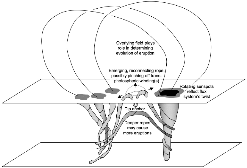
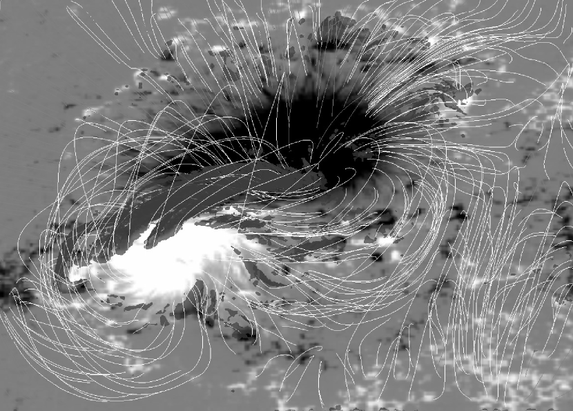
Figure 1: Top: Schematic representation for an emerging field configuration involved in flaring or flux-rope eruption as discussed in Sect. 2.2. Bottom: NLFF field model over an active region prior to an X3.4 flare (case 8 in Table 1), rendered from a perspective 50 degrees from the normal view. The two main spots are connected by a flux rope with strong electrical currents (shown by a grey isosurface) within which field lines spiral from end to end on the photosphere. The Hinode vector-magnetic data and the extensive NLFFF modeling are discussed by Schrijver et al. (2008). See Sect. 5 for a discussion of NLFFF modeling capabilities.

First, a large active region emerges, itself already carrying substantial net twist, helicity, and electrical currents, as witnessed by surface motions such as rotating sunspots, by its net kinetic helicity, and by the generally complex shape of the magnetic field.

Subsequently, a current-carrying bundle of magnetic flux (either a single flux rope, or an ensemble of such ropes, perhaps formed by pre-emergence fragmentation) breaches the solar surface (see Fig. 1-top). This rope may be a separate rise of flux through the convective envelope, or may be a late emergence of strands of flux from the same parent flux bundle that formed the active region. One flux rope, or a series of them, may emerge, forming a strong-gradient polarity-inversion line (SPIL) characterized by two parallel opposite-polarity ridges of line-of-sight flux in close proximity. At high resolution, the vector magnetic field across the SPIL will be highly sheared, and rotating as the flux bundle moves through the photosphere.

Interaction with the near-surface convection, radiative cooling in the stratified atmosphere, and the draining of heavy plasma into surface-crossing undulations or windings of the field appear to result in a number of ’anchor’ points for the emerging flux rope(s). Near-surface reconnection (“tether cutting”) enables the rope to break any ties to the interior between its two extremities, so that part or all of it can rise relatively freely into the overlying corona.

Models lead to the hypothesis that a rope may be unstable, and accelerate into an eruption, often associated with flaring, if the strength of the pre-existing field decreases rapidly enough with height (Sect. 9). Part of all of the emerged strands may participate in this, depending on the remaining sub-photospheric anchors. If the field gradient slows with height or changes sign, the flux rope may stabilize again, resulting in a confined flare or failed flux-rope (and, often, filament) eruption. If the field gradient is large (particularly if the field goes through a null, as in the “breakout” concept), the eruption may proceed higher, if not in fact into the heliosphere as a CME. If the winding of the emerging flux rope is too strong, then (confined or ejective) kinking may happen after any photospheric anchors between the end points are released; such kinking may, but needs not, transition to an ejective eruption.

Subsequent emergence of a series of flux rope fragments is likely responsible for repeating and homologous flares, which can manifest themselves as leaving non-potential energy (or helicity, or electrical currents, or filaments, …) behind in the corona if these are not (yet) unstable or released from their photospheric anchors. Or they may manifest themselves as repeating flares when subsequent strands of the flux rope emerge.

How general is this scenario? The following sections address various aspects of this, but let me point out here, in summary, that the vast majority of major flares are associated with flux emergence (within the preceding day or so) in the form of tightly wound flux ropes in active regions with large-scale twist, that field gradients above the zone near the polarity-inversion line help differentiate confined from ejective filament eruptions, while the photospheric differences between immediately before and after the flare are generally so subtle they are detected only for the largest flares that have been observed at high cadence and then only after careful inspection (Sect. 8.1). Conversely, no major flares occur in regions that have a largely potential appearance, or more than about a day after the emergence of substantial flux ropes (Sect. 9). It remains unclear what role tether-cutting or anchor-cutting play in near-photospheric reconnection (Sect. 11). These processes have both observational and theoretical support, but it remains unclear how instrumental they are in the triggering of flares, either by themselves or in combination with the (evolving) field gradient above the polarity-inversion line (Sect. 9).

3 Flares and eruptions: confined, failed, ejective

Flares, filament eruptions, and coronal mass ejections (CMEs) are three aspects that manifest themselves following the destabilization of the coronal magnetic field. Their precise relationship remains an area of intense study, which is aided by the ever-increasing observational coverage of the Sun and inner heliosphere, yet hampered by the fact that different observatories are involved that generally do not have overlapping fields of view, and in many cases do not have continuous coverage of a given target active region. Another problem is, of course, that the sources of CMEs that originate on the far side of the Sun cannot be observed, while there is ambiguity in differentiating front-side CMEs from far-side CMEs – at least there was until the launch of the STEREO spacecraft late in 2006.

In addition to flares and CMEs, there are the ’failed eruptions’ in which filaments begin to rise, but then stop their progress while twisting and writhing (see, e.g., Gilbert et al. 2007, for a discussion of this phenomenon and further references) within the confines of what appears to be a domain of connectivity for the field bounded by a separatrix; some particularly well-observed examples of this with TRACE are cases $1-7$ in Table 1. These failed eruptions are associated with flares up to low M class. At least some of these failed eruptions have no CME counterpart (e.g., Ji et al. 2003).

Table 1: Sample flaring regions and flare events discussed in the text.

No.	Time, flare magnitude	Notes	Sect.
1	2003/05/02 02:47 M1.0	Apparently failed filament eruption obs. by TRACE/171Å.	3
2	2002/05/27 18:00 M2.0	Apparently failed filament eruption obs. by TRACE/195Å.	3
3	2001/08/01 18:30 —	Apparently failed filament eruption obs. by TRACE/171Å.	3
4	2001/04/15 21:59 C5.1	Apparently failed filament eruption obs. by TRACE/171Å.	3
5	2000/11/05 00:17 C5.4	Apparently failed filament eruption obs. by TRACE/171Å.	3
6	1999/10/20 05:53 M1.7	Apparently failed filament eruption obs. by TRACE/171Å.	3
7	1999/05/31 22:10 —	Apparently failed filament eruption obs. by TRACE/171Å.	3
8	2006/12/13 02:40 X3.4	Extensive NLFFF modeling by Schrijver et al. (2008).	5
9	2008/08/25 16:23, X5.3	Ribbons distant from main PIL within AR complex.	5
10	2004/07/16 13:49, X3.6	Ribbons distant from main PIL within AR complex.	5
11	2001/04/10 05:06, X2.3	Ribbons distant from main PIL within AR complex.	5
12	2001/10/19 00:47, X1.6	Ribbons distant from main PIL within AR complex.	5
13	2003/03/18 11:51, X1.5	Ribbons distant from main PIL within AR complex.	5
14	2000/06/07 15:34, X1.2	Ribbons distant from main PIL within AR complex.	5
15	2004/07/16 10:32, X1.1	Ribbons distant from main PIL within AR complex.	5
16	2002/08/21 05:28, X1.0	Ribbons distant from main PIL within AR complex.	5
17	2004/07/17 07:51, X1.0	Ribbons distant from main PIL within AR complex.	5
18	2001/06/15T10:01 M6.3	Ribbons in adjacent AR at $\sim$5 arcmin.	5
19	2002/03/14T01:38 M5.7	Ribbons in adjacent AR at $\sim$2 arcmin.	5
20	2002/07/31T01:39 M1.2	Sympathetic flare in AR 4 arcmin. away.	5
21	2005/09/07-17 10X, 24M	AR 10808: 10 X-class and 24 M-class flares.	6
22	2003/10/18-11/05 11X	AR 10486: 11 X-class flares, including a record X28.	6
23	2000/11/24-27 5X, 2M	AR 9236: 5X and at least 2 M-class flares.	6
24	1999/09/19 08:40	Post-event arcade above a residual filament (TRACE/171 Å)	6
25	2000/07/19 23:39 —-	Erupting filament with decreasing twist (TRACE/171Å)	8.2

See http://trace.lmsal.com/POD/bigmovies/ for a collection of TRACE movies.

The fraction of flares that is associated with CMEs increases rapidly as we go from small flares to large X-class flares, reaching close to 100% for the largest ones. For example, Wang and Zhang (2007) find that 90% of 104 studied X-class flares are associated with eruptions, and Yashiro et al. (2005) find that the fraction of flares associated with CMEs increases from 20% for C3-9 flares to 100% for flares above X3. Andrews (2003) finds that 40% of M-class flares and all X-class flares in his sample are associated with CMEs.

It remains unclear precisely what determines whether a large flare is associated with a successful ejection or with a failed eruption. One clue is found in a study by Wang and Zhang (2007), who find that the 10% of X-class flares that they find not to be associated with CMEs tend to occur closer to the magnetic center of gravity of the region, leading them to suggest that eruptive flares lie closer to the periphery of the active regions. Another distinction, suggested by Nindos and Andrews (2004), may be the field’s helicity or net electrical current: they find that the best-fit linear force-free (LFF) fields have a value of the twist parameter $\alpha$ that is statistically larger in CME-producing flaring regions than in those in which the flares are not associated with CMEs, although there is substantial overlap in the samples. It is not clear what such LFF fits measure, though; a NLFFF formalism would have been appropriate, but that, too, is fraught with problems (Sect. 5).

Larger (brighter and often hotter) flares tend to be associated with faster and/or wider CMEs (which presumably tend to be more energetic); see, for example, Kay et al. (2003), Yashiro et al. (2005), Guo et al. (2007), and Georgoulis (2008). Moreover, the fastest CMEs originate in active regions. For example, Wang and Zhang (2008) find that 90% of the fastest 0.5% of CMEs (with speeds above $1500$ km/s) originate in active regions. This suggests that the energy in the surrounding magnetic field is involved in determining whether a filament eruption develops into an ejection. Other aspects are the geometry and gradient of the overlying field – see Sects. 4 and 9.

4 Flare statistics from large to small

The energy that is released during flares is converted into non-thermal particle populations, thermal populations, and bulk kinetic motion in case of ejecta. Although the initial release partitions the energy over the thermal and non-thermal particle populations (see, e.g., Krucker and Lin 2005, Saint-Hilaire and Benz 2005, and references therein), much of the non-thermal population is eventually converted into thermal energy and into the radiation that we see as the X-ray flare. Measurements of the radiative losses during flares (using, e.g., peak fluxes or fluences) thus capture much of the flare’s energy release, apart from the bulk kinetic energy in ejections and the escaping particle populations.

Despite this incomplete access to the total energy involved in flares and eruptions, many studies suggest that peak fluxes or fluences are among the useful metrics for flaring activity. Distribution functions of estimated energies of solar flares can be approximated by power laws rather well (see, e.g., the overview in Table I in Aschwanden et al. 1998, who review flare statistics from hard X-rays to radio as well as energetic particle events; see also Su et al. 2006, for an analysis of RHESSI flares; and Hudson 2007, for a compilation of 32 years of GOES $1-8$Å flares). Figure 2 summarizes the flare-energy power laws from nano- to X-class flares (with energies of ${\cal O}(10^{31-32})$ ergs).

The existence of power laws in not limited to flares. Robbrecht (2007) finds essentially a power-law distribution for the widths of CMEs. Flares with or without CMEs may be statistically different: Yashiro et al. (2006), for example, suggest that power-law distributions for peak fluxes, fluences, and duration are significantly steeper for flares without CMEs than for flares associated with CMEs. On the other hand, Wheatland (2003) reports that the waiting-time distribution for CMEs is like that of a time-dependent Poisson process, similar to that found for flares observed in the GOES records.

Figure 2: Distribution functions for estimated flare energies derived from observations in the extreme ultraviolet, soft X-rays, and hard X-rays. The energy range in this diagram spans eight orders of magnitude. From Aschwanden et al. (2000).

In reviewing the evidence for the common occurrence of power laws for flare properties, Charbonneau et al. (2001) conclude that their existence “suggests that the flaring process is intrinsic to coronal magnetic fields, even though the flaring rate may be controlled by extrinsic factors, such as magnetic flux emergence in the photosphere.” The inference that the power-law distribution of flare properties may reflect some intrinsic property of the corona is consistent with the finding that the same power-law distributions are found when looking at subsets of flares from particular regions: Wheatland (2000b) shows that the distributions of peak flare strengths for individual active regions is consistent with the joint pdf for all regions, and concludes that, apart from the frequency, ’the statistics of flares appear to be independent of the physical characteristics of the originating active regions’, at least within the statistical uncertainties. A study by Kucera et al. (1997) supported an upper-limit to flare magnitudes dependent on the region’s spot coverage (cf., Sect. 7). They also found a reduced number of small flares in regions with high spot coverage, but suggest that an observational bias in their data requires further study on that issue; Wheatland (2000b) finds no significant evidence for such an effect.

Hudson (2007) comments on the predictability of X-class flares from a cycle perspective. He points out that the frequency of these events through three solar cycles does not follow the Poisson statistics based on metrics for the sunspot cycle that appear applicable to lesser flares: there are more major flares in the cycle-minimum phases than there ought to be if their occurrence scaled simply with active-region frequency. The flaring frequency appears rather specific to active region properties and their sub-photospheric sources, and these appear to change with the cycle in ways that remain to be uncovered.

The statistical commonality of the shape (apart from the overall frequency) of the flare-energy spectrum for all regions has led to the introduction of the concept of the ’avalanche model’ or ’self-organized criticality’ (SOC; see, e.g., the review by Charbonneau et al. 2001) in which the size of a flare is only statistically determined, and in which the flare’s energy is always much less than the available total energy (thus allowing repeating and homologous flares with little change in the boundary field, see Sect. 5). The SOC of the coronal field may develop as a consequence of the processes that inject the non-potential energy into the active-region coronae - discussed further in the following sections. We have to wonder, though, whether the ’self-organization’ reflects a coronal property or is rather a property of the subsurface processes that supply the energy in the first place (see Sect. 10). With that in mind, let me now proceed with a discussion of what we know - or rather what we do not know - about flare energetics based on field measurements.

5 Field models and topology, free energy, and helicity

Models of solar flares would have free energy in excess of a lower-energy field to which it can relax, (relative) helicity, and field topology play important roles in determining whether a flare can occur, where it will begin its development, and what the final state of the coronal magnetic field can be. In order to derive such properties, ideally one would like to model the coronal field in detail based on the observable boundary conditions in the low atmosphere.

The electrical currents in the solar atmospheres above flare-prone active regions are substantial, and we know that such currents can lead to significant changes in field geometry (see Sect. 9) and topology (e.g., Hudson and Wheatland 1999). Unfortunately, modeling the coronal field has turned out to be exceedingly difficult. Problems abound (see, e.g., Klimchuk et al. 1992, McClymont et al. 1997, Schrijver et al. 2006a, Metcalf et al. 2006, Metcalf et al. 2008; Schrijver et al. 2008, and DeRosa et al. 2009): nonlinear force-free field (NLFFF) models or virial-theorem applications based on photospheric vector fields (that are subject to problems of their own, including inversion problems and an intrinsic 180^∘ ambiguity for the transverse field) have to be developed further if they are to provide reliable estimates of the free energy, relative helicity, or topology. Schrijver et al. (2008) illustrate this very clearly. They compare field models for AR 10930 (case no. 8 in Table 1) based on high-quality Hinode/SP vector-magnetic measurements, using a variety of NLFFF algorithms and a range of boundary conditions. Only one of these solutions approximates the observed coronal configuration (bottom panel in Fig. 1). A subsequent study by DeRosa et al. (2009) based on Hinode and STEREO observations concludes that there is, as yet, no successful strategy for NLFFF modeling that can be applied under general circumstances to yield significant energy estimates and reliable field geometries. Consequently, in my opinion, we have yet to succeed to a level that makes comparison of observation-based field models with theoretical concepts valuable to differentiate between different flare scenarios.

When studying the changes in field properties from before to after a flare, an added problem to the one discussed above is that the volumes that can be effectively modeled within computational limitations are so small that they have no real solar counterparts that may be considered to be closed to any physical quantity. Hence, the apparent convenience of having a conserved quantity - the relative helicity - can in reality not be exploited effectively, even if it could be reliably measured.

Then there is, of course, the problem that the coronal field is anchored in the photosphere (which shows only subtle lasting changes during the course of a flare, see Sect. 8.1), which limits the field’s relaxation towards a LFF field. Moreover, in any given flare, only part of a region’s helicity and energy may be involved (see Sect. 7). Consequently, even if we were able to measure the ’free energy’ in excess of either a potential field or a LFF field (at the same or any other relative helicity), we would only be able to place an upper limit on the magnitude of a flare.

Those studies that do try to measure energy or helicity in spite of the above problems, typically find that the energy or relative helicity in the region suffices to power a flare or CME, and that they typically decrease from before to after the flare, even when measuring relative to a LFF field at the same helicity (e.g., Bleybel et al. 2002; Metcalf et al. 2005; Régnier and Canfield 2006; Régnier and Priest 2007a [also Régnier and Priest 2007b]; Bobra et al. 2008; Liu 2007). Perhaps we can have more confidence in relative measurements than in absolute measurements? Or perhaps we are establishing that flares release only a small fraction of the total energy associated with the field, so that we should not be surprised that the energy in a (N)LFF field model exceeds the potential or LFF-field energy by enough to let us conclude that there is enough energy to power the flare. That would be a rather more spurious result than one would like to have.

The application of the virial theorem to the lower-boundary field suffers from its own problems. For example, Wheatland and Metcalf (2006) argue that the virial estimates of the free energy in active region fields based on the surface vector field can be somewhat improved over the simple boundary where that ignores Lorentz forces, but that the results are subject to very substantial uncertainties. An application of the virial theorem to a model field in the detailed study by Metcalf et al. (2008), for example, shows that the magnitude of the uncertainty in the virial-theorem estimate of free energy is comparable to that in NLFF models.

If we cannot, yet, rely on measurements based on field models, can we at least rely on the overall geometry of the field, and in particular properties of its skeleton, such as (quasi-)separatrices? For nearly potential fields, this should be possible, but the largest flares and CMEs are associated with decidedly non-potential fields (see Sect. 9), which unfortunately cannot be successfully modeled. For example, Hudson and Wheatland (1999) point out that the observation that flares occur primarily at separatrices (or quasi-separatrix layers) is largely unproven because of the mapping ambiguities in 3D field models. Where such agreements are found, we should probably even question whether that is because in such cases the non-potentiality (or force-free parameter $\alpha$) is rather small, so that we are largely looking at the properties of a potential-field configuration.

One property of flares that has proven quite telling as far as the reconnected field involved is the phenomenon of flare ribbons. They have long been associated with impact sites of energetic particles caused by reconnection (for one detailed study on this, see Asai et al. 2003). Generally, flare ribbons consist of partially- or fully-outlined fronts moving away on either side of a pronounced polarity inversion line; see, e.g., Fletcher and Hudson 2001, and Fletcher et al. 2005, for discussions of particular events, with references to other studies). They are interpreted as the signatures of reconnection following the eruption of field through an arcade-like overlying field, leading to particle acceleration and precipitation, energy thermalization, and thus eventually to the two-ribbon flare observable in visible light, UV, and EUV. In the case of a true ejection of a (frequently filament-carrying) flux rope into interplanetary space, one would expect that the erupting field has to break through more than the lowest domain of connectivity for the field, and that consequently more ’ribbons’ should show up than only the innermost ones (which is likely to be the brightest and most readily observable one). It seems that this phenomenon of more distant particle impact sites has received relatively little attention, perhaps because of the problem of limited fields of view, perhaps because their interpretation requires a large-scale field model that is generally not available. Nevertheless, a study of such events (of which I list some examples in Table 1, cases $9-19$) may prove quite telling on large-scale field topology and its changes, and should be much easier with the full-Sun field of view of the future Solar Dynamics Observatory. Studies of such larger areas may also shed light on the phenomenon of the sympathetic flare (an example of which is case no. 20 in Table 1).

Li et al. (1997) find that hard X-ray flare footpoints occur preferentially at the edges of channels of strong vertical currents as inferred from vector-magnetograms. This is suggestive of reconnection between a current-carrying rope and its surrounding field at flare onset (cf., Sect. 8.1). Higher-resolution Hinode data are well suited for a follow-up of that work, once the cycle picks up strength.

Initial flare brightenings, whether in ribbons or in more compact impact sites or compact flaring sites, generally lie close to the primary, strongest polarity-inversion line: Schrijver (2007) find that the average distance $D$ of the brightest TRACE (E)UV location at flare onset (the first brightening within about 1 ksec from the GOES flare start time, often shown by the EUV diffraction pattern associated with the filter support grid) to the nearest point on a SPIL within the region is 20 Mm. The distribution of $D$ is strongly peaked at small distances, such that about 70% of the flares have $D<15$ Mm, compared to a typical scale for the active regions of at least 150 Mm. Such distance measurements can be used in combination with detailed models, as in the study by Gary and Moore (2004), who discuss a filament eruption in which the initial brightenings lie relatively far enough from the polarity-inversion lines that they argue this is evidence for the initial reconnections to lie above, rather than below the erupting filament. I return to the role of SPILs in Sect. 7 and to the merits of ’breakout’ and ’tether-cutting’ concepts involved in the argument of Gary and Moore in Sect. 9.

6 Homology and repeaters

Among the potentially telling properties of flares we find the phenomenon of repeating flares for a given active region, and in particular the sub-category of the homologous flare. In homologous flares very nearly the same site and flare ribbons are involved in sequences of two or more flares. Among the well-studied regions of repeated flaring, we find, for example, AR 9236, AR 10808 (among the most flare-productive regions recorded based on the GOES soft X-ray data), and AR 10486 (see entries $21-23$ in Table 1).

The repeating (possibly homologous) flare suggests that either not all of the available energy is released in a flare, or that energy continues to be supplied to the region so that a series of flares of various magnitudes can occur. Evidence is found for both of these possibilities. For example, Bleybel et al. (2002) study a case in which the post-flare configuration remains inconsistent with a LFFF model (either based on the pre-event or the post-event relative helicity as determined by a Grad-Rubin based NLFFF code). Multiple studies have reported on continued flux emergence between successive homologous flares (see, for example, Ranns et al. 2000; Nitta and Hudson 2001; Sterling and Moore 2001; Takasaki et al. 2004; and Dun et al. 2007). Some of these repeater events clearly show that not all the available energy is taken away in an event. One such example is that of case 24 in Table 1 which shows a post-eruption arcade over a residual filament structure.

Some studies argue that systematic motions, such as the persistent rotation of sunspots, are involved in rebuilding the energy for homologous flares (see also Sect. 10), such as Zhang et al. (2008) (see also the related numerical model by DeVore and Antiochos 2008). The phenomenon of the rotating sunspot is generally associated with ongoing flux emergence, however (such as in the case of the X17.2 flare Oct. 28, 2003, one of the subjects of Zhang et al. 2008, part of entry 22 in Table 1), and without flux emergence, major flares rarely, if at all, occur (see Sect. 8). Besides, it is hard to estimate whether flux emergence or spot rotation adds most energy (e.g., Régnier and Canfield 2006) in view of the discussion in Sect. 5. The reformation of loop systems involved in long-distance, even trans-equatorial connections (Khan and Hudson 2000) is harder to interpret, but perhaps also hinting that not all energy is removed during eruptive events.

Figure 3: Scatter diagram of peak flare flux densities (GOES $1-8$ Å passband in W/m²) versus the absolute total flux near the strong-field, high-gradient polarity inversion, $R$ (in relative units). The histograms in this figure show the 25-th, 50-th, and 75-th percentiles of the flare distribution as function of $R$. The dotted straight line at $F_{\rm peak}=1.2\times 10^{-8}\,R$ has 99% of the observed flares below it. The only flare that clearly lies above this line is an X6.2 flare that started around 2001/12/13 14:30 UT. The value of $\log{(R)}$ in this active region decreased from 4.2 half a day prior to the flare to 3.7 at the time of the flare, but at 4.2 would still lie well above the dotted line. This region has a narrow fibril of one polarity embedded within an area of strong field of the opposite polarity, which likely causes the measure $R$ to strongly underestimate the true flux involved (see footnote). This may (in part) explain its unusual position in this diagram. From Schrijver (2007).

7 Patterns in the surface field

The most frequently used observable of the magnetic field involved in impulsive and eruptive events is the surface line-of-sight field, largely because it is readily measured (and has been, routinely, for a long time). Increasingly, vector-magnetic measurements have become available. Often, the frequency of either of these measurements is rather low, in part because of observational limitations for ground-based observatories. Consequently, many studies have focused on finding properties of patterns of the surface magnetic field in snapshot line-of-sight magnetograms that might shed light on the powering and triggering of impulsive phenomena.

One type of study focuses on statistical properties of the magnetic field of active regions. First, it appears that M- and X-class flares occur in sunspot-containing regions with very few exceptions. The work of, e.g., Dodson and Hedeman (1970) and Ruzdjak et al. (1989) points out that whereas flares do occur in spotless regions, these account for only about 2% of all flares while the largest documented flare in soft X-rays of this type was classified as M1.2. This is the only documentated case I found for which a major flare in soft X-rays occurred in a spotless region; all of the 289 M- and X-class flares, for example, that were studied by Schrijver (2007) – which were the basis of the study resulting in Fig. 3 – have spots associated with them.

Another statistical property was pointed by by Canfield and Russell (2007), who find that a tessellation of active-region magnetograms at a few arc-second resolution yields log-normal distributions, suggesting that the flux bundles were subjected to repeated random fragmentation during their rise to the surface (compare the study by Bogdan 1985, on a similar size distribution of spot areas). They find no significant correlation between the degree of fragmentation and either the flare rate of the active regions or the mean density of kinetic helicity, concluding that it is more likely that large-scale helicity in the flow is related to flaring than small-scale interactions between convection and rising flux. On the other hand, Abramenko (2005) finds that the indices of power spectra of the photospheric magnetic field of flare-prone regions increase from $-1.7$ for flare-quiet up to as steep as $-2.3$ for regions producing high X-class flares (see her Fig. 5). It is not clear how the preceding two results are to be reconciled.

Some of the salient features in the active-region magnetic field have received far more attention than the above-mentioned statistical properties, in particular the properties of the polarity-inversion lines. Despite all this attention, no measure (either single or combined) has been identified as being particularly well correlated with the flare activity of active regions. For example, Georgoulis (2008) studies 23 eruptive active regions and finds that for active regions with ’intense polarity inversion lines’ (as measured by a metric that combines fluxes and field-line lengths from connectivity matrices between positive and negative fluxes in magnetograms) tend to have both stronger flares and faster CMEs. Wang and Zhang (2008) find that the length and number of the polarity-inversion lines (PILs) are good indicators of fast vs. slower CMEs. The findings by Falconer et al. (2006) (expanding on Falconer et al., 2002, 2003) suggest a more complex dependency: for a sample of active regions with one well-defined, dominant polarity-inversion line they find that several measures are correlated similarly to the region’s flare potential. These measures include the length of the strong-shear segment of the PIL, the length of the main PIL with a strong field gradient across it, the total net current, and the best-fit $\alpha$ from a LFF field based on a comparison of the photospheric vector field with the model field footprint. They suggest that the best metric for the total magnetic free energy is, in fact, a combination of total flux and total twist.

The ambiguity in findings in general is likely in part the result of the correlation between multiple parameters, and disentangling these requires large statistical samples. The study by Leka and Barnes (2007) is an excellent example of that, but still leaves us with an unclear picture. They analyze 496 active regions to establish which parameters of the photospheric field are most successful in differentiating flaring from non-flaring regions. They measure 28 different properties from the vector-magnetic field measurements and differentiate flaring from non-flaring regions within 24 h of these magnetograph observations. Their discriminant analysis has a success rate of 93% for M1 flares or larger (compared to 91% when simply labeling all regions as flare-quiet, see Sect. 12), or 80% for C1 or larger (compared to 70% in the absence of any information on the region). They find that the best-performing single parameter for large flares is a proxy for the magnetic free energy in the region; other top performers are variables that measure the field’s various properties integrated over the entire active region.

Table 2: Likelihood of X or M flares within 24 h of the determination of the unsigned magnetic flux ${\cal R}$ within about 15 Mm of high-gradient, strong-field polarity-separation lines (see Schrijver, 2007, for a detailed description and normalization factor). The likelihoods are sampled at 0.5 dex intervals, but vary smoothly with ${\cal R}$. Also listed is the maximum expected flare class.

$\log{(\cal R)}=$	$<$3.0	3.0	3.5	4.0	4.5	5.0
$>$M1	0%	2%	5%	12%	50%	$\sim$80%
$>$M3	0%	$\sim$0%	$<$1%	3%	20%	35%
$>$X1	0%	0%	$\sim 0$%	$\sim$1%	10%	20%
$>$X3	0%	$0$%	$0$%	$\sim 0$%	1%	$1-2$%
Maximum:	$<$C9	$<$M1	$<$M4	$<$X1	$<$X4	$<$X10

Another example of a statistical study is that by Schrijver (2007), who looks at the magnetic properties of regions associated with almost 300 M- and X-class flares, and compares that with the properties of 2,500 randomly selected active regions, all within 45^∘ of disk center. He notes that the regions with large flares all have a pronounced polarity-inversion line with a strong gradient across it. He subsequently measures the unsigned flux ${\cal R}$ within about 15 Mm of such strong PILs (SPILs), and this is a good indicator for flares that allows prediction of the largest flare to be expected from the region (see Fig. 3 and Table 2; I return to the issue of predictability and the skill of various metrics in Sect. 12).

Based on the inspection of many full-disk SOHO-MDI magnetogram sequences for regions with large flares, Schrijver (2007) argues that the SPILs appear to be associated with emerging flux, in particular with emerging flux ropes (also supported by the detailed field modeling by Schrijver et al. 2008; cf. Fig. 1). Welsch and Li (2008) show that there is a pronounced tendency of increasing ${\cal R}$ to be correlated with increasing total unsigned flux, i.e., with signs of flux emergence. Given the resolution of full-disk MDI magnetograms and the likelihood that emerging flux immediately cancels partly against pre-existing flux, this is strong evidence for flux emergence as driver for the SPIL flux metric ${\cal R}$. More evidence for the association with flux ropes in particular is found when looking at shear at such SPILs.

Shear at the polarity-inversion line is often associated with flaring activity (examples are a statistical study by, e.g., Cui et al. 2007, and individual event studies by Kurokawa et al. 2002, Brooks et al. 2003, Dun et al. 2007, Schrijver et al. 2008, Okamoto et al. 2008, and Lites 2008; also coronal field studies described in Sect. 9). The same holds for eruptions: Vrsnak et al. (1991) report that the pitch angle of H$\alpha$ structures outlining filaments is telling regarding the eruption potential: prominences with twist angles exceeding 50^∘ and heights exceeding 80% of the footpoint separation erupted, while those with angles below 35^∘ and heights below 60% of the footpoint separation were stable.

Manchester (2007), based on simulations of an emerging flux rope, argues that shear motion at the polarity-inversion line in emerging flux is a natural consequence of the Lorentz forces that develop as a rope enters the corona. This may explain the general correspondence of field shear and shear flows.

8 Flare-related changes in the magnetic field

8.1 Before and after in the photosphere

The conversion of large-scale electromagnetic energy in the process of a flare or filament eruption changes the field configuration over active regions, and this should in turn have consequences for the observable vector-magnetic field in the photosphere. Until recently, these changes proved elusive (other than temporary changes in line profiles during the flares, which are mostly if not entirely a consequence of the energy deposition in the near-atmospheric layers by populations of energetic particles generated early in the flare, see, e.g., Schrijver et al. 2006b).

Part of the problem in finding flare-related field changes is that it cannot really be done with vector-magnetic measurements based on spectrograph scans, simply because these scans take too long to complete relative to the evolution of the photospheric field between two successive magnetograms with spacings that are much longer than the impulsive phase of the flare or eruption. For example, Dun et al. (2007), using a series of 12 vector-magnetograms in the course of five days of AR 10486 (case 22 in Table 1), find that magnetic shear angles, electric current density, and current helicity increase at the sites of impulsive flares at least a day prior to the main (X17 and X10) flares. But they attribute these changes to the emergence of twisted flux ropes rather than to changes associated with the flares per se. Although they say their metrics decrease after the main flares, the observational cadence is too low to unambiguously differentiate flare-related relaxation of the field or the passage of flux ropes through the photosphere prior to the post-flare magnetograms.

The analysis of line-of-sight magnetograms taken at much higher frequency has been successful in identifying differences in the magnetic field just before and after major flares. Sudol and Harvey (2005), for example, find: a) that the time scale for changes in the l.o.s. field is less than $\sim 10$ min., some even less than one minutes, but in all cases abrupt; b) in many cases these changes are close to the noise but in some cases very significant; c) the changes persist for at least the two hours past the peak flare time studied by them, and in one case for at least 5 hours. They note that most of these observed field changes occur in spot penumbrae, and that for the three flares for which TRACE coverage is available, these changes occur at sites of flare ribbons in the (E)UV. The authors argue that these field changes are lasting, and thus likely not the result of atmospheric changes related to the particle impact or heat conduction leading to the flare-ribbon formation; perhaps the energy deposition occurs (very nearly) along the current-carrying field lines involved in a reconnection event. The fact that these field changes are often close to the detection threshold even for major flares will make it difficult for field modelers to reliably deduce changes in the field energy from before to after flares in general – see Sect. 5).

Wang et al. (1994) show cases in which the shear angle across the polarity-inversion line of active regions increases during, and persists after a set of five X-class flares, with a time resolution that ranges from about 4-10 min. in the best cases to about 45 min. They propose as one possible interpretation that new flux emerging just before the flare could be the cause of this increase, but comment that it is hard to understand how that could change the shear over more than 10,000 km in such a short time. On the other hand, Chen et al. (1994) report on shear studies of 18 regions around M-class flares; they find no detectable changes, suggesting that perhaps only the largest flares are associated with observable changes.

Even very large flares and eruptions are associated with relatively weak or very localized changes in the surface magnetic field. This is, of course, part of the problem of measuring significant changes in the field energy, helicity, and topology around the time of such field destabilizations: too often, the field changes that are reported are mixed in with intrinsic changes in the photospheric field caused by flows (horizontal and, often, vertical associated with flux emergence) owing to the substantial time intervals between successive magnetograms, thus masking the changes associated with the flare or eruption only. The potential of, e.g., the 1-min. cadence magnetogram sequences for SOHO/MDI has not yet been utilized. Moreover, we shall need sensitive (vector-) magnetographs, preferably for the chromospheric field, with high cadences and sizable fields of view in order to learn about vector field changes at the lower boundary at times of flares and eruptions.

8.2 Before and after in the corona

There do not seem to be many studies that compare the coronal appearance before and well after a major flare (well observed in, e.g., case 24 in Table 1). There are some studies, however, that look at loops early in a flare/eruption and in the late stages of the post-flare arcade. Among these is Asai et al. (2003), who find that during the course of the initial stages of the flare, the conjugate footpoints at first indicate strongly sheared field lines, and later reveal less sheared coronal connections. Su et al. (2007a) study TRACE observations of 50 X- and M-class two-ribbon flares, with well-defined, largely parallel ribbons. They find that 86% of these flares show a general decrease in the shear angle between the main polarity inversion line and pairs of conjugate bright ribbon kernels. They interpret this as a relaxation of the field towards a more potential state because of the eruption that carries helicity/current with it, but one can readily argue that a similar decrease in shear angle would be seen if sequentially higher, less-sheared post-flare loops lit up with time as the loops cool after reconnection. These results are consequently ambiguous: they may show a decrease in shear, or they may reflect that flares generally do not release all available energy and part of the flux-rope configuration remains (cf., Sect. 6).

Su et al. (2007b), from a study of a sample of 31 two-ribbon flares with CMEs, find that the primary parameters describing the peak flare brightness and CME terminal velocity are the total flux in the region, and the change in shear angle between the early and late phases of the flare, and - to a significantly lesser degree - the initial shear angle. The change in shear angle may reflect a real decrease in shear and associated energy, but - in view of the preceding paragraph - may also be a measure of the residual shear after the eruption; hence, it remains unclear what the measured shear angle is telling us in this case.

Compounding the efforts to understand the field evolution are the relative roles of twist and writhe, and their coupling. One study on this topic by Romano et al. (2003) reports that the number of turns around an erupting filament initially is about 5, decreasing to 1 later into the eruption (entry 25 in Table 1). Here we may see an exchange of twist and writhe.

9 The overlying coronal field

Numerical MHD models continue to shed light on the potential causes of the instability that leads to flares and, in particular, filament eruptions, as always with the clear caveat that such modeling is an approximating abstraction of reality. Some of these models rely on the expected general slowness of reconnection in a solar atmospheric plasma, except for particular field configurations, specifically null points. The so-called breakout model, for example, “exploits a vulnerability of multi-polar configurations, which consist of two or more distinct flux systems separated by null points in the corona, to rearrangements of the magnetic field’s connectivity” (DeVore and Antiochos 2008). Specifically, rapid reconnection is anticipated as flux is pushed into a null region. One recent example of such fields is discussed by DeVore and Antiochos (2008). They simulate a multi-polar configuration with a null in the corona over a model active region subjected to rotational flows (somewhat like rotating sunspots). Their simulation run extends to cover three homologous eruptions in their breakout concept. These, by the way, are confined, in the sense that they erupt only from the active region, but not into interplanetary space.

Another concept is the ’tether-cutting’ model (originally described by Moore and Roumeliotis 1992), in which (near-)photospheric reconnection associated with flux emergence removes the ’anchors’ to flux rope that can subsequently reconnect with the overlying field, or even erupt. This is discussed further in Sect. 11.

A different possibility to destabilize a field configuration is related to the kink and torus instabilities. The kink instability occurs when the helicity, current, or winding-number for the field in a flux rope exceeds a critical value. For example, Fan and Gibson (2004) perform line-tied MHD simulations of an emerging flux rope into a pre-existing configuration. For a case in which the twisted field in the top part of the rising rope has the same general direction as the overlying arcade, they find that the configuration becomes unstable after the coronal field reaches 1.76 full turns about the rope’s axis. The erupting rope exchanges twist for writhe as it evolves as is often - but certainly not always - seen in filament eruptions. In a case in which the rope’s top-most winding relative to the overlying arcade is reversed, no flux rope builds up in the corona as reconnection proceeds from the very first emergence, and consequently no instability develops.

The torus instability occurs whenever the gradient in the surrounding field is strong enough, so that the forces exerted on a flux rope subject to a perturbation cannot be contained by the overlying magnetic field. Kliem and Török (2006) (also, e.g., Fan and Gibson 2007) discuss the torus instability, and find a critical field gradient beyond which the configuration is unstable. They argue that line tying of the field to the photospheric boundary in this case helps to stabilize a configuration, arguing that it may even stabilize an emerging flux rope entirely until it is semi-circular and thereafter may help to destabilize it.

Török and Kliem (2007) discuss a unifying approach to slow and fast CMEs in which the torus instability drives the CME, and in which the gradient in the surrounding field determines the acceleration profile and eventual velocity of the ejecta: fast CMEs for rapid decrease (as typical of ARs) and slow for gradual decrease (as often over quiet Sun). Isenberg and Forbes (2007) start from a similar field configuration as developed by Titov and Démoulin (1999), but perform an analytical analysis for eruptions without twist (i.e., without the subsurface current introduced by Titov and Démoulin 1999). They confirm the instability of the configuration when the flux rope length exceeds a few times the diameter of the flux rope.

Following the proposition of the torus instability, Wang and Zhang (2007), based on potential-field models, find that ’the ratio of the magnetic flux in the low corona to that in the high corona is systematically larger for the eruptive events than for the confined ones’. Liu (2008), for a sample of ten flares, find a low field gradient for failed eruptions or kinking, and a steeper gradient for successful eruptions. The power-law indices for the field decrease with height for the failed eruptions and for the kink and torus eruptions combined are $-1.62\pm 0.05$ and $-1.91\pm 0.15$, respectively, for height ranges from $\log(h[{\rm km}])=3.7-4.7$. The use of potential-field models here is an oversimplification and the findings may say more about the distribution of the surrounding field on the photosphere than about the actual field gradient in the low corona.

The above-mentioned studies deal with CMEs in which flux ropes that may contain filaments are part of the story. It remains to be seen how this can apply to flares, or to eruptions with failed ejections, but there is no obvious reason why the above arguments would not apply to compact flares as much as they do to more extended flux-rope cum filament systems.

In view of the theoretical and numerical considerations described in the preceding subsection, it is no surprise that multiple observational studies look at the coronal field configuration. Of course, this brings us back to the problem that the coronal magnetic field configuration cannot be known really well with present tools (Sect. 5). This is particularly bothersome because it is clear that the coronal fields in flare-prone regions differ markedly from the potential field based on the same vertical (or line of sight) photospheric field; see, for example, Schrijver et al. (2005). This does not mean that currents pervade much of the active-region corona, of course, but at least points out that somewhere there must be currents strong enough to warp the field relative to a pure potential field everywhere from the core field to the peripheral field. It appears that such currents survive for typically only a day, while powering one or more flares during their decay (e.g., Pevtsov et al. 1994; Burnette et al. 2004; Schrijver et al. 2005).

How common is a strongly non-potential field? Burnette et al. (2004) compare photospheric vector-magnetograms and coronal configurations as seen by YOHKOH’s SXT. They compute LFF models that best match the coronal geometry, and find that over 90% of the regions studied are fitted well by such a model. Nindos and Andrews (2004) find that this is true for only 60% of their sample. Furthermore, Burnette et al. (2004) find that the $\alpha$ parameter derived from the vector-magnetogram correlates well with that estimated for the coronal configuration. Apparently, the currents that are responsible for the large-scale non-potentiality of the coronal field close through the photosphere, while small-scale structure of the $\alpha$ parameter in the photosphere often does not contribute significantly to the large-scale field configuration.

The electrical currents involved in non-potential regions appear to emerge with the flux, according to several studies. Pevtsov et al. (2003), for example, use line-of-sight MDI magnetograms and LFF field fits to EIT EUV images to estimate the helicity evolution in emerging active regions. They find that the helicity parameter $\alpha$ starts essentially at zero on first emergence for all six regions that were well observed, and subsequently converges to a maximum plateau value over the following 1.5 d. They argue that this means that the twist is in fact injected into the corona by ’the spinning of the active region polarities driven by magnetic torque from below’. Note that this means on first emergence, the coronal field is apparently nearly potential, with $\alpha\sim 0$. Work by Longcope and Welsch (2000) supports this finding.

The studies in the literature, both observational and theoretical, suggest that whether a flux rope erupts not at all, evolves into a “failed eruption”, or makes it into the heliosphere as a CME depends critically on the structure of the overlying field, in particular on the gradient of the field with height, but likely also the direction of the overlying field relative to the twist of the emerging flux rope.

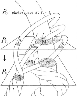
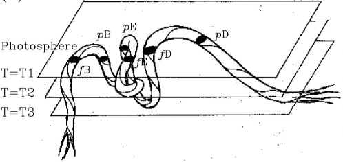
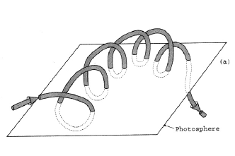
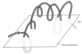
Figure 4: Select examples of proposed 3D configurations to explain the motions of pores around a spot (top left), of the complex motions of multiple concentrations of flux in an emerging region (top right), and the photospheric crossing of an emerging flux rope (bottom two panels). In these sketches the possibility of efficient supra-photospheric reconnection (as in the Ellerman bombs of Fig. 5) has been ignored. (Top left: from Ishii et al., 1998; top right: Kurokawa et al., 2002; bottom: from Low, 2001)

10 Subsurface processes, emerging flux, and rotating spots

Currents through the photosphere are often not neutralized when integrating over either of the two polarities. It has been argued (e.g., Melrose 1991, Melrose 1995, Wheatland 2000a) that consequently these currents cannot have been induced by non-current carrying flux emergence, because in that case the currents should balance within each polarity. Hence, instead, at least some of these currents must have emerged from below the photosphere. This notion is compatible with the observational evidence that the Sun’s magnetic field is often twisted on emergence (e.g., Kurokawa 1987, Tanaka 1991 [see, e.g., his Fig. 5], Leka et al. 1996, van Driel-Gesztelyi et al. 1997, Ishii et al. 1998, López Fuentes et al. 2000, Okamoto et al. 2008). Brooks et al. (2003) study in detail, with high spatio-temporal resolution, the conditions of two emerging flux regions, one with a small flare, and one without, in the field of view of the SVST. They find that the flaring region is associated with the emergence of what looks like a twisted, i.e., current-carrying flux rope (compare Fig. 1), while the other has no such appearance.

Not only emerging currents contribute to a region’s free energy, however. Also systematic flow patterns at, or just below, the surface can do so. For example, Nightingale et al. (2007), report that rotating sunspots are associated with almost all of the X-flares observed by TRACE since April 1998, and many of the M-flares.

It is difficult to differentiate twist in the emerging flux from twisting flows. Support that these twists are associated with flows, at least below the surface, is found by Komm et al. (2005), who estimate the kinetic helicity density (${\bf v}\cdot{\bf\nabla}\times{\bf v}$) below active regions using helioseismic measurements. They find that the maximum helicity density in the outer 2% of the Sun correlates ’remarkably well’ with the X-ray flaring activity, perhaps - as they point out - because of the link between helicity and twist in the subsurface magnetic field.

Whereas sunspot rotation has been argued to add energy to the coronal field, either because of the work done by the (sub-)photospheric flows or because it reflects the emergence of a twisted, current-carrying flux bundle, the study by Schrijver (2007) shows that all X-M flaring regions contain SPILs. As all X-flaring regions appear to contain rotating sunspots, it may well be that these are related phenomena, perhaps because many, if not all, flux bundles in a flare-prone region have significant electrical currents associated with them induced by preferential flow systems.

There appears to be a net relative helicity in each hemisphere, negative in the north, positive in the south, corresponding to left-handed screws in the north and right-handed ones in the south: the statistical study by Pevtsov et al. (1995) shows a 2:1 preferences of the sign of helicity for the hemispheres, averaged over all latitudes and for two cycles (see Longcope and Pevtsov 2003). This twist, if existent already below the surface, is likely to be affected by turbulent convective buffeting of rising flux (see López Fuentes et al. 2000, for a discussion of an example of this). As Longcope and Pevtsov (2003) argue, this would trade twist with writhe of the emerging flux tubes, without affecting relative helicity. The writhe should affect the tilt angle of dipole axes on emergence, if not cause kinking of the subsurface flux arches into what may be seen as complex, or even $\delta$-class regions. This suggestion has been made, but I have not found this empirically investigated.

On the theoretical side, a persistent problem is that even state-of-the-art numerical experiments still have difficulty in successfully bringing flux bundles from some depth up into the photosphere without them exploding in the strongly stratified uppermost layers of the convective envelope (e.g., Fan 2004). Note that among the stabilizing forces in this process we find increasing curvature, the Coriolis forces, and Reynolds number (e.g., Abbett et al. 2000, Abbett et al. 2001, Magara 2006, Cheung 2006). Models suggest that twist is needed for the flux bundles - thus turning them into flux ropes - to survive the rise. On the other hand, it appears that modelers need to impose more twist than warranted by observations, as most active regions emerge with archfilament systems mostly aligned with the eventual dipole axis of the region rather than nearly perpendicular to it as in many simulations (e.g., Archontis et al. 2005; Magara 2006; Manchester 2007; Fan 2008).

Starting with too much twist subjects the emerging flux ropes to kink instabilities. Fan (2008) discusses models of rising flux tubes through a rotating medium stratified like a convective envelope. She shows that if these non-axisymmetric flux tubes rise with a twist of the observed hemispheric preference that is strong enough to prevent substantial shredding during the rise, the twist converts into a writhe that has the opposite sign than the observed preferred tilt angle. If the twist is weakened by only a factor of two this effect becomes weaker than that of the Coriolis force, and the net result is a tilt that is comparable to the observed one. But the consequence of this is that the rising 3D tube loses a lot of its flux by shredding as it moves buoyantly through the surrounding medium. In view of this, one sees this scenario develop: weakly twisted tubes explode and cause network field; moderately twisted regions have a trail of shredded field behind them, perhaps causing active-region nesting; and strongly twisted field should come up coherently, perhaps subjected to a kinking-instability leading to $\delta$-spots.

11 The role of near-photospheric reconnection

With mounting evidence for the emergence of flux ropes as a characteristic ingredient in major solar flaring, it is instructive to look at some of the highest-resolution studies made of the process of flux emergence. These observations suggest that emerging magnetic flux often does not emerge as a simple arch, as traditionally studied, but rather as an undulating field that transits the photospheric layer multiple times in sea-serpent fashion. In such a geometry, the magnetic field reaching into the chromosphere might drain its plasma load into sub-photospheric dips in the field, with trapped material that would not allow those field segments to rise. But perhaps near-surface reconnection allows the heavily mass-loaded pockets of magnetic field to be pinched off (thus creating a variant of the tether-cutting concept in which the emerging and pre-existing flux ropes are, in fact, one and the same).

Lites (2008) discusses such observations of emerging flux made with Hinode’s SP, NFI, and BFI. He argues that the observations of opposite-polarity patches moving towards each other, with downflows seen in the spectral data, present an opportunity for plasma to drain back into the photosphere, and then be pinched off from the supra-photospheric configuration, which can then rise into the corona. Recent numerical simulations of emerging flux (e.g., Cheung et al. 2008) support such an interpretation.

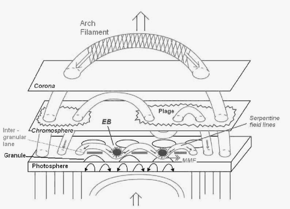
Figure 5: Conceptual illustration (by Schmieder and Pariat, 2007) of emerging flux, with undulating strands of flux with multiple photospheric crossings. In this concept, the approach of pairs of corresponding opposite-polarity patches on either side of a dipped field line could lead to reconnection (in what might appear as an Ellerman bomb, or EB) that pinches off the heavy sub-photospheric segment, thus allowing the flux to rise. For field configurations that can destabilize, twist and or kinking appears needed, as illustrated in Figs. 1 and 4.

The concept of pinching off the heavy, sub-photospheric dips in emerging, twisted magnetic field (such as sketched in the lower panels of Fig. 4) has been suggested before (also, e.g., Pariat et al. 2004). One example of this is the interpretation of Ellerman bombs as shown in Fig. 5, taken from Schmieder and Pariat (2007).

12 Instability, catastrophe, and predictability

Let me, finally, address two issues before ending this review. First a comment on the nature of the instability. We have to ask whether this instability can be the result of a bifurcation that occurs in certain conditions under which there is more than one state for the field to be in given the observed photospheric vector field. The existence of more than one field configuration for the same lower boundary could be the explanation for why lasting photospheric changes from pre- to post-flare states are hard to find (although they have been reported on, see Sect. 8.1). Not much seems to have been written on this topic, but interestingly, Isenberg and Forbes (2007) point out that they ’have found evidence that each T&D [Titov and Démoulin 1999] equilibrium has a corresponding toroidal equilibrium with exactly the same boundary conditions at the solar surface, which is unstable when the T&D equilibrium is stable and vice versa,’ thus pointing to a catastrophe scenario. Among the other studies that address the existence of multiple solutions (some stable, some unstable) I mention the catastrophe models by van Ballegooijen and Martens (1989) and Forbes and Isenberg (1991). Whether the possibility that the nearly force-free state of the coronal field allows multiple solutions to (very nearly) the same boundary condition will need additional work in order to be able to assess these effects in the context of field instabilities.

The second point relates to the predictability based on proposed metrics for flare likelihood. A landmark study in this is the work by Barnes and Leka (2008) who evaluate the skill scores of forecasts based on four metrics: total flux, the “total excess energy” (Leka and Barnes 2003), the SPIL flux metric ${\cal R}$ (Schrijver 2007), and the “effective connected magnetic field” (Georgoulis and Rust 2007). They limit their sample to regions within 30^∘ from disk center to create a relatively uniform set of observing conditions. They show that the highest success rate for any of these single parameter, ${\cal R}$, is 92.2%, whereas a uniform forecast that nothing will every produce an M-class flare or larger is 90.8%. They conclude that none of these parameters are robust as forecasting tools.

13 In conclusion – looking forward

This, then, brings us back to the issue of “understanding.” If we could deterministically forecast flares and eruptions, then we certainly could claim success. But we might also have reached a deep understanding if this were not the case: if flux-rope emergence is the driver, or if self-organization occurs within the corona, then no such thing as a “deterministic forecast” based on present-day observables is feasible in principle. How do we find out if either or both of these possibilities apply? It seems that statistical studies for observations from interior to high corona are essential. The relatively slow process of emergence and the rapidity of flare onset also point to multi-day, high-cadence coverage for such coordinated observations.

These observations need to be complemented by numerical experiments of flux emergence with a realistic treatment of the interior, of the near-surface layers, and of the corona. Moverover, we shall need to learn how to model the atmospheric field in order to measure properties such as energy, helicity, and topology.

Coordinated multi-instrument observations of the Sun in the era of the Solar Dynamics Observatory, supported by extensive spectroscopy and numerical experiments, hold the promise of a breakthrough for our understanding of magnetic instabilities involved in flares and CMEs.

Acknowledgments.

I thank Hugh Hudson, Nariaki Nitta, and Alan Title for very helpful comments on early drafts of this manuscript, and the referees for very constructive suggestions to improve the presentation and to some key references.

References

- Abbett et al. (2000) Abbett, W. P., G. H. Fisher, and Y. Fan: 2000. ApJ 540, 548.
- Abbett et al. (2001) Abbett, W. P., G. H. Fisher, and Y. Fan: 2001. ApJ 546, 1194.
- Abramenko (2005) Abramenko, V. I.: 2005. ApJ 629, 1141.
- Andrews (2003) Andrews, M. D.: 2003. Solar Phys. 218, 261.
- Archontis et al. (2005) Archontis, V., F. Moreno-Insertis, K. Galsgaard, and A. W. Hood: 2005. ApJ 635, 1299.
- Asai et al. (2003) Asai, A., T. T. Ishii, H. Kurokawa, T. Yokoyama, and M. Shimojo: 2003. ApJ 586, 624.
- Aschwanden et al. (1998) Aschwanden, M. J., B. R. Dennis, and A. O. Benz: 1998. ApJ 497, 972.
- Aschwanden et al. (2000) Aschwanden, M. J., T. D. Tarbell, R. W. Nightingale, C. J. Schrijver, A. M. Title, C. C. Kankelborg, P. C. H. Martens, and H. P. Warren: 2000. ApJ 535, 1047.
- Barnes and Leka (2008) Barnes, G. and K. D. Leka: 2008. Solar Phys. submitted.
- Bleybel et al. (2002) Bleybel, A., T. Amari, L. van Driel-Gesztelyi, and K. D. Leka: 2002. A&A 395, 685.
- Bobra et al. (2008) Bobra, M. G., A. A. van Ballegooijen, and E. E. DeLuca: 2008. ApJ 672, 1209.
- Bogdan (1985) Bogdan, T. J.: 1985. ApJ 299, 510.
- Brooks et al. (2003) Brooks, D. H., H. Kurokawa, K. Yoshimura, H. Kozu, and T. E. Berger: 2003. A&A 411, 273.
- Burnette et al. (2004) Burnette, A. B., R. C. Canfield, and A. A. Pevtsov: 2004. ApJ 606, 565.
- Canfield and Russell (2007) Canfield, R. C. and A. J. B. Russell: 2007. ApJL 662, L39.
- Charbonneau et al. (2001) Charbonneau, P., S. W. McIntosh, H.-L. Liu, and T. J. Bogdan: 2001. Solar Phys. 203, 321.
- Chen et al. (1994) Chen, J., H. Wang, H. Zirin, and G. Ai: 1994. Solar Phys. 154, 261.
- Cheung (2006) Cheung, M.: 2006, ‘Magnetic flux emergence in the solar photosphere’. Ph.D. thesis, Max Planck Inst. for Solar System Research, Lindau, for Univ. Würzburg.
- Cheung et al. (2008) Cheung, M. C. M., M. Schüssler, T. D. Tarbell, and A. M. Title: 2008. ApJ. in press.
- Cui et al. (2007) Cui, Y., R. Li, H. Wang, and H. He: 2007. Solar Phys. 242, 1.
- DeRosa et al. (2009) DeRosa, M., C. Schrijver, G. Barnes, K. Leka, B. Lites, M. Aschwanden, T. Amari, A. Canou, J. McTiernan, S. Regnier, J. Thalmann, G. Valori, M. Wheatland, T. Wiegelmann, M. Cheung, P. Conlon, M. Fuhrmann, B. Inhester, and T. Tadesse: 2009. ApJ. in preparation.
- DeVore and Antiochos (2008) DeVore, C. R. and S. K. Antiochos: 2008. ApJ 680, 740.
- Dodson and Hedeman (1970) Dodson, H. W. and E. R. Hedeman: 1970. Solar Phys. 13, 401.
- Dun et al. (2007) Dun, J., H. Kurokawa, T. T. Ishii, Y. Liu, and H. Zhang: 2007. ApJ 657, 577.
- Falconer et al. (2002) Falconer, D. A., R. L. Moore, and G. A. Gary: 2002. ApJ 569, 1016.
- Falconer et al. (2003) Falconer, D. A., R. L. Moore, and G. A. Gary: 2003. JGR (Space Physics) 108(A10), 1380.
- Falconer et al. (2006) Falconer, D. A., R. L. Moore, and G. A. Gary: 2006. ApJ 644, 1258.
- Falconer et al. (1997) Falconer, D. A., R. L. Moore, J. G. Porter, G. A. Gary, and T. Shimizu: 1997. ApJ 482, 519.
- Fan (2004) Fan, Y.: 2004. Living Reviews in Solar Physics 1, 1.
- Fan (2008) Fan, Y.: 2008. ApJ 676, 680.
- Fan and Gibson (2004) Fan, Y. and S. E. Gibson: 2004. ApJ 609, 1123.
- Fan and Gibson (2007) Fan, Y. and S. E. Gibson: 2007. ApJ 668, 1232.
- Fisher et al. (1998) Fisher, G., D. Longcope, T. Metcalf, and A. Pevtsov: 1998. ApJ 508, 885.
- Fletcher and Hudson (2001) Fletcher, L. and H. Hudson: 2001. Solar Phys. 204, 71.
- Fletcher et al. (2005) Fletcher, L., J. A. Pollock, and H. E. Potts: 2005. Solar Phys. 222, 279.
- Forbes and Isenberg (1991) Forbes, T. G. and P. A. Isenberg: 1991. ApJ 373, 294.
- Gary and Moore (2004) Gary, G. A. and R. L. Moore: 2004. ApJ 611, 545.
- Georgoulis (2008) Georgoulis, M. K.: 2008. Geophys. Res. Lett. 35, 6.
- Georgoulis and Rust (2007) Georgoulis, M. K. and D. M. Rust: 2007. ApJL 661, L109.
- Gilbert et al. (2007) Gilbert, H. R., D. Alexander, and R. Liu: 2007. Solar Phys. 245, 287.
- Guo et al. (2007) Guo, J., H. Q. Zhang, and O. V. Chumak: 2007. A&A 462, 1121.
- Hudson (2007) Hudson, H. S.: 2007. ApJL 663, L45.
- Hudson and Wheatland (1999) Hudson, T. S. and M. S. Wheatland: 1999. Solar Phys. 186, 310.
- Isenberg and Forbes (2007) Isenberg, P. A. and T. G. Forbes: 2007. ApJ 670, 1453.
- Ishii et al. (1998) Ishii, T. T., H. Kurokawa, and T. T. Takeuchi: 1998. ApJ 499, 898.
- Ji et al. (2003) Ji, H., H. Wang, E. J. Schmahl, Y.-J. Moon, and Y. Jiang: 2003. ApJL 595, L135.
- Kay et al. (2003) Kay, H. R. M., L. K. Harra, S. A. Matthews, J. L. Culhane, and L. M. Green: 2003. A&A 400, 779.
- Khan and Hudson (2000) Khan, J. I. and H. S. Hudson: 2000. Geophys. Res. Lett. 27, 1083.
- Kliem and Török (2006) Kliem, B. and T. Török: 2006. Physical Review Letters 96(25), 255002.
- Klimchuk et al. (1992) Klimchuk, J. A., R. C. Canfield, and J. E. Rhoads: 1992. ApJ 385, 327.
- Komm et al. (2005) Komm, R., R. Howe, F. Hill, I. González Hernández, and C. Toner: 2005. ApJ 630, 1184.
- Krucker and Lin (2005) Krucker, S. and R. P. Lin: 2005. In: F. Favata, G. Hussain, and B. Battrick (eds.): 13th Cambridge Workshop on Cool Stars, Stellar Systems, and the Sun. pp. 101–106, ESA SP-560.
- Kucera et al. (1997) Kucera, T. A., B. R. Dennis, R. A. Schwartz, and D. Shaw: 1997. ApJ 475, 338.
- Kurokawa (1987) Kurokawa, H.: 1987. Solar Phys. 113, 259.
- Kurokawa et al. (2002) Kurokawa, H., T. Wang, and T. T. Ishii: 2002. ApJ 572, 598.
- Leka and Barnes (2003) Leka, K. D. and G. Barnes: 2003. ApJ 595, 1277.
- Leka and Barnes (2007) Leka, K. D. and G. Barnes: 2007. ApJ 656, 1173.
- Leka et al. (1996) Leka, K. D., R. C. Canfield, A. N. McClymont, and L. van Driel-Gesztelyi: 1996. ApJ 462, 547.
- Li et al. (1997) Li, J., T. R. Metcalf, R. C. Canfield, J.-P. Wuelser, and T. Kosugi: 1997. ApJ 482, 490.
- Lites (2008) Lites, B. W.: 2008. In: A. Balogh (ed.): ISSI proceedings of a workshop on the solar dynamic magnetic field.
- Liu (2007) Liu, Y.: 2007. Adv. Space Res. 39, 1767.
- Liu (2008) Liu, Y.: 2008. ApJL 679, L151.
- Longcope and Pevtsov (2003) Longcope, D. W. and A. A. Pevtsov: 2003. Adv. Space Res. 32, 1845.
- Longcope and Welsch (2000) Longcope, D. W. and B. T. Welsch: 2000. ApJ 545, 1089.
- López Fuentes et al. (2000) López Fuentes, M. C., P. Demoulin, C. H. Mandrini, and L. van Driel-Gesztelyi: 2000. ApJ 544, 540.
- Low (2001) Low, B. C.: 2001. JGR 106, 25141.
- Magara (2006) Magara, T.: 2006. ApJ 653, 1499.
- Manchester (2007) Manchester, W. I.: 2007. ApJ 666, 532.
- McClymont et al. (1997) McClymont, A. N., L. Jiao, and Z. Mikić: 1997. Solar Phys. 174, 191.
- Melrose (1991) Melrose, D. B.: 1991. ApJ 381, 306.
- Melrose (1995) Melrose, D. B.: 1995. ApJ 451, 391.
- Metcalf et al. (2008) Metcalf, T. R., M. L. Derosa, C. J. Schrijver, G. Barnes, A. A. van Ballegooijen, T. Wiegelmann, M. S. Wheatland, G. Valori, and J. M. McTtiernan: 2008. Solar Phys. 247, 269.
- Metcalf et al. (2006) Metcalf, T. R., K. D. Leka, G. Barnes, B. W. Lites, M. K. Georgoulis, A. A. Pevtsov, K. S. Balasubramaniam, G. A. Gary, J. Jing, J. Li, Y. Liu, H. N. Wang, V. Abramenko, V. Yurchyshyn, and Y.-J. Moon: 2006. Solar Phys. 237, 267.
- Metcalf et al. (2005) Metcalf, T. R., K. D. Leka, and D. L. Mickey: 2005. ApJL 623, L53.
- Moore and Roumeliotis (1992) Moore, R. L. and G. Roumeliotis: 1992. In: Z. Svestka, B. V. Jackson, and M. E. Machado (eds.): IAU Colloq. 133: Eruptive Solar Flares, Vol. 399 of Lecture Notes in Physics, Berlin Springer Verlag. p. 69.
- Nightingale et al. (2007) Nightingale, R. W., A. P. Ji, and S. A. Mayo: 2007. AGU Fall Meeting Abstracts p. A1112.
- Nindos and Andrews (2004) Nindos, A. and M. D. Andrews: 2004. ApJL 616, 175.
- Nitta and Hudson (2001) Nitta, N. V. and H. S. Hudson: 2001. Geophys. Res. Lett. 28, 3801.
- Okamoto et al. (2008) Okamoto, T. J., S. Tsuneta, B. W. Lites, M. Kubo, T. Yokoyama, T. E. Berger, K. Ichimoto, Y. Katsukawa, S. Nagata, K. Shibata, T. Shimizu, R. A. Shine, Y. Suematsu, T. D. Tarbell, and A. M. Title: 2008. ApJL 673, L215.
- Pariat et al. (2004) Pariat, E., G. Aulanier, B. Schmieder, M. K. Georgoulis, D. M. Rust, and P. N. Bernasconi: 2004. ApJ 614, 1099.
- Pevtsov et al. (1994) Pevtsov, A. A., R. C. Canfield, and T. R. Metcalf: 1994. ApJL 425, 117.
- Pevtsov et al. (1995) Pevtsov, A. A., R. C. Canfield, and T. R. Metcalf: 1995. ApJL 440, L109.
- Pevtsov et al. (2003) Pevtsov, A. A., V. M. Maleev, and D. W. Longcope: 2003. ApJ 593, 1217.
- Ranns et al. (2000) Ranns, N. D. R., L. K. Harra, S. A. Matthews, and J. L. Culhane: 2000. A&A 360, 1163.
- Régnier and Canfield (2006) Régnier, S. and R. C. Canfield: 2006. A&A 451, 319.
- Régnier and Priest (2007a) Régnier, S. and E. R. Priest: 2007a. ApJL 669, L53.
- Régnier and Priest (2007b) Régnier, S. and E. R. Priest: 2007b. A&A 468, 701.
- Robbrecht (2007) Robbrecht, E.: 2007. In: On-line proceedings of an LWS workshop: http://www.lmsal.com/lws2007/programoverview.html.
- Romano et al. (2003) Romano, P., L. Contarino, and F. Zuccarello: 2003. Solar Phys. 214, 313.
- Ruzdjak et al. (1989) Ruzdjak, V., B. Vrsnak, R. Brajsa, and A. Schroll: 1989. Solar Phys. 123, 309.
- Saint-Hilaire and Benz (2005) Saint-Hilaire, P. and A. O. Benz: 2005. A&A 435, 743.
- Schmieder and Pariat (2007) Schmieder, B. and E. Pariat: 2007. Scholarpedia 2(12), 4335. http://www.scholarpedia.org/article/Magneticfluxemergence.
- Schrijver et al. (2008) Schrijver, C., M. DeRosa, T. Metcalf, G. Barnes, B. Lites, T. Tarbell, J. McTiernan, G. Valori, T. Wiegelmann, M. Wheatland, T. Amari, G. Aulanier, P. Démoulin, M. Fuhrmann, K. Kusano, S. Régnier, and J. Thalmann: 2008. ApJ 675, 1637.
- Schrijver (2007) Schrijver, C. J.: 2007. ApJL 655, 117.
- Schrijver et al. (2005) Schrijver, C. J., M. L. De Rosa, A. Title, and T. R. Metcalf: 2005. ApJ 628, 501.
- Schrijver et al. (2006a) Schrijver, C. J., M. L. DeRosa, T. R. Metcalf, Y. Liu, J. McTiernan, S. Régnier, G. Valori, M. S. Wheatland, and T. Wiegelmann: 2006a. Solar Phys. 235, 161.
- Schrijver et al. (2006b) Schrijver, C. J., H. S. Hudson, R. J. Murphy, G. H. Share, and T. D. Tarbell: 2006b. ApJ 650, 1184.
- Sterling and Moore (2001) Sterling, A. C. and R. L. Moore: 2001. JGR 106, 25227.
- Su et al. (2006) Su, Y., W. Q. Gan, and Y. P. Li: 2006. Solar Phys. 238, 61.
- Su et al. (2007a) Su, Y., L. Golub, and A. A. Van Ballegooijen: 2007a. ApJ 655, 606.
- Su et al. (2007b) Su, Y., A. Van Ballegooijen, J. McCaughey, E. Deluca, K. K. Reeves, and L. Golub: 2007b. ApJ 665, 1448.
- Sudol and Harvey (2005) Sudol, J. J. and J. W. Harvey: 2005. ApJ 635, 647.
- Takasaki et al. (2004) Takasaki, H., A. Asai, J. Kiyohara, M. Shimojo, T. Terasawa, Y. Takei, and K. Shibata: 2004. ApJ 613, 592.
- Tanaka (1991) Tanaka, K.: 1991. Solar Phys. 136, 133.
- Titov and Démoulin (1999) Titov, V. S. and P. Démoulin: 1999. A&A 351, 707.
- Török and Kliem (2007) Török, T. and B. Kliem: 2007. Astronomische Nachrichten 328, 743.
- van Ballegooijen and Martens (1989) van Ballegooijen, A. A. and P. C. H. Martens: 1989. ApJ 343, 971.
- van Driel-Gesztelyi et al. (1997) van Driel-Gesztelyi, L., G. Csepura, B. Schmieder, J.-M. Malherbe, and T. Metcalf: 1997. Solar Phys. 172, 151.
- Vrsnak et al. (1991) Vrsnak, B., V. Ruzdjak, and B. Rompolt: 1991. Solar Phys. 136, 151.
- Wang et al. (1994) Wang, H., M. W. Ewell, Jr., H. Zirin, and G. Ai: 1994. ApJ 424, 436.
- Wang and Zhang (2007) Wang, Y. and J. Zhang: 2007. ApJ 665, 1428.
- Wang and Zhang (2008) Wang, Y. and J. Zhang: 2008. ApJ 680, 1516.
- Welsch and Li (2008) Welsch, B. T. and Y. Li: 2008. In: R. Howe, R. W. Komm, K. S. Balasubramaniam, and G. J. D. Petrie (eds.): Subsurface and Atmospheric Influences on Solar Activity, Vol. 383 of Astronomical Society of the Pacific Conference Series. p. 429.
- Wheatland (2000a) Wheatland, M. S.: 2000a. ApJ 532, 616.
- Wheatland (2000b) Wheatland, M. S.: 2000b. ApJ 532, 1209.
- Wheatland (2003) Wheatland, M. S.: 2003. Solar Phys. 214, 361.
- Wheatland and Metcalf (2006) Wheatland, M. S. and T. R. Metcalf: 2006. ApJ 636, 1151.
- Yashiro et al. (2006) Yashiro, S., S. Akiyama, N. Gopalswamy, and R. A. Howard: 2006. ApJL 650, 143.
- Yashiro et al. (2005) Yashiro, S., N. Gopalswamy, S. Akiyama, G. Michalek, and R. A. Howard: 2005. JGR (Space Physics) 110(A9), 12.
- Zhang et al. (2008) Zhang, Y., J. Liu, and H. Zhang: 2008. Solar Phys. 247, 39.