Achieving Perfect Imaging beyond Passive and Active Obstacles by a Transformed Bilayer Lens

Abstract

A bilayer lens is proposed based on transformation optics. It is shown that Pendry’s perfect lens, perfect bilayer lens made of indefinite media, and the concept of compensated media are well unified under the scope of the proposed bilayer lens. Using this concept, we also demonstrate how one is able to achieve perfect imaging beyond passive objects or active sources which are present in front of the lens.

PACS numbers: 41.20-q, 42.79.Bh, 42.25.Bs

The form-invariance property of the Maxwell’s equations in any coordinate system P1 ; Ulf1 ; Ulf2 provides us a convenient guideline to design the so-called transformation media for controlling electromagnetic (EM) fields or light in an unprecedented manner. In this design methodology, a coordinate transformation function describes the desired trajectory of EM field in a direct geometrical meaning Ulf1 , and it determines the material parameters of the transformation media by tensor rules P1 ; Ulf1 . The most intriguing application of the theory is invisibility cloak, as proposed by Pendry et al P1 and Leonhardt et al Ulf2 in their preliminary works. Since then, this particular field of study, referred to as transformation optics, has received intense attention from the optics community. We have so far observed a surge of theoretical discussions Cai ; Cum ; Ruan ; Chen1 ; Ulf3 ; Yan and even experimental efforts Sch related especially to the cloaking subject. Apart from invisibility cloaks, some other novel applications of transformation optics, such as, beam shifters and splitters Rahm , field rotation Chen2 , and electromagnetic wormholes Gf , have been proposed.

In Refs. [9], it is shown that a Pendry’s perfect slab lens P2 with $n=-1$ can be interpreted by transformation optics. In particular, the lens body together with its free space background can be considered as transformation media obtained from a coordinate transformation of free space based on a folded mapping function. Following this strategy, a perfect cylindrical (spherical) shape lens can be designed by deploying a folded radial spatial mapping in a cylindrical (spherical) coordinate system YM2 . On the other hand, Pendry’s perfect slab lens can be understood as a special example of compensated media P3 . In this paper, by studying a transformed bilayer structure, we notice that transformation optics provides a clear physical interpretation of such compensated media, the compensated media are just special examples of the transformed, in particular, bilayer structure. Thus, we can define a generalized concept of compensated media, which well unify Pendy’s slab lens and the indefinite media lens proposed by Smith et al Smith ; Sch2 . Based on this understanding, we show that perfect imaging can be realized even when passive obstacles or active emitters are obstructing our object to be imaged.

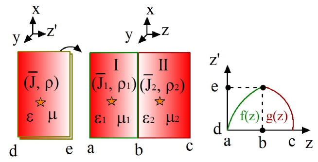
Figure 1: Illustration of a bilayer slab structure obtained by coordinate transformations from a single slab layer.

Consider a coordinate transformation which transforms a single slab structure placed in EM space into a bilayer slab structure, as illustrated in Fig. 1. The single slab structure in EM space has relative permittivity $\epsilon$ and relative permeability $\mu$, and may contain active sources denoted by $\overline{J}$ and $\rho$. The transformation function is also illustrated in Fig. 1. It is seen that the region $z^{{}^{\prime}}\in[d,e]$ in EM virtual space transforms into two regions $z\in[a,b]$ and $z\in[b,c]$ in physical space following transformation functions $z^{{}^{\prime}}=f(z)$ and $z^{{}^{\prime}}=g(z)$, respectively. The two transformation functions have the boundary conditions $f(a)=g(c)=d$ and $f(b)=g(b)=e$. The material parameters as well as sources in the transformed layers, denoted by layer I and layer II, can be expressed as P1 ; Ulf1

$$\varepsilon_{1}=\det(\Lambda_{f})^{-1}\Lambda_{f}\varepsilon\Lambda_{f},\;\mu_{1}=\det(\Lambda_{f})^{-1}\Lambda_{f}\mu\Lambda_{f},$$ (1)

$$\varepsilon_{2}=\det(\Lambda_{g})^{-1}\Lambda_{g}\varepsilon\Lambda_{g},\;\mu_{2}=\det(\Lambda_{g})^{-1}\Lambda_{g}\mu\Lambda_{g},$$ (2)

$$\overline{J}_{1}=\det(\Lambda_{f})^{-1}\Lambda_{f}J,\;\rho_{1}=\det(\Lambda_{f})^{-1}\rho,$$ (3)

$$\overline{J}_{2}=\det(\Lambda_{g})^{-1}\Lambda_{g}J,\;\rho_{2}=\det(\Lambda_{g})^{-1}\rho,$$ (4)

where $"\det"$ represents the determinant of a matrix, $\Lambda_{f}=diag[1,1,1/f^{{}^{\prime}}(z)]$ and $\Lambda_{g}=diag[1,1,1/g^{{}^{\prime}}(z)]$.

If the fields in the layer I are denoted by $\overline{E}_{1}(x,z)$ and $\overline{H}_{1}(x,z)$, based on transformation optics, the fields in the layer II should be related to the fields in the layer I by

$$\overline{E}_{2}(x,y,z)=diag[1,1,g^{{}^{\prime}}(z)/f^{{}^{\prime}}(z_{m})]\overline{E}_{1}(x,y,z_{m}),$$ (5)

$$\overline{H}_{2}(x,y,z)=diag[1,1,g^{{}^{\prime}}(z)/f^{{}^{\prime}}(z_{m})]\overline{H}_{1}(x,y,z_{m}),$$ (6)

where $z\in[b,c]$ and $z_{m}\in[a,b]$ correspond to the same $z^{{}^{\prime}}$ . At boundaries $z=a$ and $z=c$, we have $\overline{E}_{2}(x,c)=diag[1,1,h^{{}^{\prime}}(c)/g^{{}^{\prime}}(a)]\overline{E}_{1}(x,a)$ and $\overline{H}_{2}(x,c)=diag[1,1,h^{{}^{\prime}}(c)/g^{{}^{\prime}}(a)]\overline{H}_{1}(x,a)$. Therefore the tangential fields at $z=a$ and $z=c$ two boundaries have the same values. The left and right outside backgrounds appear as connecting each other directly. Here, we note that this phenomenon is independent of the background material choice, or whether active sources are involved in transformation. Effectively, the two boundaries $z=a$ and $z=c$ of the bilayer are perfect duplicates of the $z^{{}^{\prime}}=d$ boundary of the original slab. Thus, if the bilayer is put into a homogenous background, the fields will perfectly tunnel through the bilayer without any reflection.

Now we examine the material properties of such a bilayer lens in general. Consider that transformation functions are linear functions with slopes being $p_{1}$ and $-p_{2}$, respectively, where $p_{1}p_{2}>0$. Thus, the thicknesses of layer I and layer II (denoted by $L_{1}$ and $L_{2}$ respectively) relate to each other by $L_{1}=\gamma L_{2}$, where $\gamma=p_{2}/p_{1}$. Observing Eqs. (5) and (6), we have $\varepsilon_{2}(x,y,z)=-\gamma diag[1,1,-1/\gamma]\varepsilon_{1}(x,y,z_{m})diag[1,1,-1/\gamma]$, $\mu_{2}(x,y,z)=-\gamma diag[1,1,-1/\gamma]\mu_{1}(x,y,z_{m})diag[1,1,-1/\gamma]$, where $z$ and $z_{m}$ are defined as the same as in Eqs. (5) and (6). When $\gamma=1$, the above equations describe exactly the complementary media proposed by Pendry in Ref. [16]. In particular, $\varepsilon_{2}(x,y,z)=-\varepsilon_{1}(x,y,z_{m})$ and $\mu_{2}(x,y,z)=-\mu_{1}(x,y,z_{m})$, if $\varepsilon_{(1,2)}$ and $\mu_{(1,2)}$ are diagonal matrices. As discussed in Ref. [16], the bilayer composed by two complimentary layers with the same thickness can transfer EM fields perfectly from one interface to the other. Here, we show that transformation optics facilitates simple and clear geometrical interpretation of the perfect lensing phenomenon of such complementary media. In fact, bilayer structure as complementary media can be extended to the following situations: (1) $\gamma\neq 1$, and/or (2) $f(z)$ and $g(z)$ are nonlinear functions, and/or (3) active sources are embedded in the bilayer.

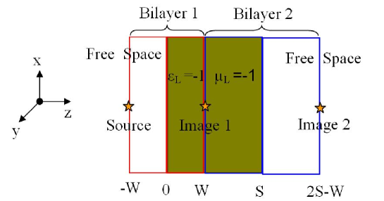
Figure 2: Illustration of Pendry’s perfect lens from the view of the bilayer structure.

As special examples, here we show how the transformed bilayer lens can encompass Pendry’s perfect lens as well as the bilayer indefinite media lens proposed by Smith et al. Consider the single slab in EM space is homogenous. With linear coordinate transformations, the individual layers of the corresponding bilayer in physical space are therefore also homogenous. If the parameters of layer I are denoted by $\epsilon_{1}=diag[\epsilon_{1x},\epsilon_{1y},\epsilon_{1z}]$ and $\mu_{1}=diag[\mu_{1x},\mu_{1y},\mu_{1z}]$, the parameters of the layer II are $\epsilon_{2}=-diag[\epsilon_{1x}\gamma,\epsilon_{1y}\gamma,\epsilon_{1z}/\gamma]$, $\mu_{2}=-diag[\mu_{1x}\gamma,\mu_{1y}\gamma,\mu_{1z}/\gamma]$. Consider Pendry’s perfect lens with $\epsilon_{1}=\mu_{1}=-1$ P2 , which is located in $z\in[0,S]$ and is put in free space background. The imaging process of this lens can be understood easily if we interpret the system as two connected bilayer structures for the billayer 1 with $\epsilon_{1}=-\epsilon_{2}=1$, $\mu_{1}=-\mu_{2}=1$ and $\gamma=1$, and the bilayer 2 with $-\epsilon_{1}=\epsilon_{2}=1$, $-\mu_{1}=\mu_{2}=1$ and $\gamma=1$, as illustrated in Fig. 2. Refer to the figure, if a source is put on the plane $z=-W$ with $W<S$, its perfect image (Image 1) will be formed at $z=W$ through perfect field tunneling by the bilayer 1. Then, through field tunneling by the bilayer 2, a perfect image 2 is constructed in free space at $z=2S-W$. Furthermore, consider the single slab in EM space is made of indefinite medium. Subject to linear coordinate transformations, the corresponding bilayer is composed by homogenous indefinite media where the material tensors $\epsilon_{(1,2)}$ and $\mu_{(1,2)}$ have both positive and negative components. In this case, we notice that such an indefinite bilayer is exactly the perfect lens made of the indefinite bilayer proposed by Smith et al. Smith ; Sch2 .

Now we give a further example of a homogenous bilayer lens located at $z\in[0,4\lambda]$ with $\epsilon_{1}=4$, $\mu_{1}=1$, $\epsilon_{2}=-4+0.008i$ and $\mu_{2}=-1+0.008i$, where $\lambda$ is the operating wavelength. The simulations are carried out with the finite-element method (FEM) using the commercial COMSOL Multiphysics package. Notice that in simulations presented in this paper, all material parameters smaller than $1$ are all given a small imaginary part of $0.008i$. This small imaginary part not only avoids the theoretical singularity problem, but also physically represents losses possessed by realistic metamaterails. The electric field distribution for a line current source $J_{s}=A\delta(z+0.01\lambda)\delta(x)$ interacting with the bilayer is plotted in Fig. 3 (a). It is seen that the EM field tunnels through the bilayer perfectly, and an almost perfect image is achieved at the exit boundary $z=4\lambda$. In Fig. 3(b), the field intensity distribution as a function of lateral position at the exit boundary $z=4\lambda$, for both with and without the bilayer, are plotted for comparison. The image constructed by the bilayer achieves a subwavelength resolution with a full width at half maximum (FWHM) of $0.28\lambda$. Whereas for the case without the bilayer, the field has decayed significantly and appears featureless.

If the single slab in EM space is inhomogeneous, the corresponding transformed bilayer will be inhomogeneous too. This hints that perfect image can be achieved even when obstacles are obstructing the object to be imaged. To illustrate this idea, we consider that a dielectric cylindrical obstacle, with a radius of $2/3\lambda$ and a refractive index of $2$, is put at at ($x=0$ $z=\lambda$), just in front of a Pendy’s lens. The lens has $\epsilon_{L}=-1+0.008i$, $\mu_{L}=-1+0.008i$, and is positioned at $z\in[0,10/3\lambda]$. The simulated electric field distribution for a line current source $J_{s}=A\delta(z+7/3\lambda)\delta(x)$ interacting with the lens and obstacle is plotted in Fig. 4(b). In Fig. 4(a), we also plot the electric field distribution when the cylindrical obstacle is absent. The Pendry’s lens is outlined by solid lines, while dashed lines outline two bilayers. Comparing Figs. 4(a) and (b), it is clearly seen that the images are distorted by the obstacle, since the up bilayer fails to transfer the field perfectly. To overcome this problem, we embed an complementary cylinder inside the lens, which has a permittivity of $-4+0.008i$ and a permeability of $-1+0.008i$. The complementary cylinder is positioned.symmetrically with the outside obstacle about $z=0$. Thus, the up bilayer works as a self-compensating bilayer lens again. In Fig. 4(c), we show the electric field distribution when the complementary cylinder is added inside the lens. Two images are constructed almost perfectly again. In Fig. 4(d), the field intensity distributions at the image plane $z=13/3\lambda$ for Figs. 4(a), (b) and (c) are plotted. It is observed that the intensity curves for (a) and (c) agree with each other quite well.

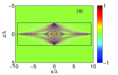
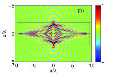
Figure 5: Electric field distribution for (a) two current sources $\overline{J}_{1}=A\delta(x)\delta(z+1.9\lambda)\hat{y}$ and $\overline{J}_{2}=-A\delta(x)\delta(z-1.9\lambda)\hat{y}$ embedded in the bilayer ; (b) only $\overline{J}_{1}$ is embedded in the bilayer. The bilayer lens has the same material parameters as in Fig. 3.

Next, we analysis the situation where active sources presented in the single layer in EM space. The transformed bilayer thus contains double amount of the mapped sources. The currents or changes of the mapped sources are determined through Eqs. (3-4). Here we assume that no other sources are present in the background. EM fields are therefore radiated only by the sources embedded in the bilayer. Thus, the power flows cross two boundaries $z=a$ and $z=c$ should be in opposite directions, i.e., outward from the bilayer. However, as discussed previously, tangential EM fields at $z=a$ and $z=c$ boundaries are always the same, which indicates that the power flows cross $z=a$ and $z=c$ should be of the same value and with the same direction. The above two conclusions are contradictory unless we acknowledge that the power flows cross $z=a$ and $z=c$ are both zero. It follows that no power flow propagates cross both $z=a$ and $z=c$. Therefore, EM fields outside the bilayer should be zero or they consist only evanescent components. However, if the fields outside the bilayer indeed consist evanescent components, they must decay in the same direction on both sides of the bilayer, since the EM tangential fields at two boundaries $z=a$ and $z=c$ have the identical values. This leads to infinite EM evanescent fields at $z=-\infty$ or $z=+\infty$, which is obviously unphysical. Hence, one comes to the conclusion that the EM fields outside the bilayer are completely zero. An outside observer can’t see any source embedded in the bilayer. As an example to illustrate this statement, we consider that a bilayer is located at $z\in[-2\lambda,2\lambda]$ which has the same material parameters as in Fig. 3(a). Two line current sources $\overline{J}_{1}=A\delta(x)\delta(z+1.9\lambda)\hat{y}$ and $\overline{J}_{2}=-A\delta(x)\delta(z-1.9\lambda)\hat{y}$ are embedded in layer I and II, respectively. The simulated electric field distribution is plotted in Fig. 5 (a). It is clearly seen that EM fields are nearly zero outside the bilayer. For a comparison, we also plot the electric field distribution when $J_{2}=0$ in Fig. 5(b), where relatively large fields outside the bilayer are observed.

Such a bilayer with active sources can be applied to design a perfect lens for achieving subwavelength imaging beyond active noise sources. To illustrate this idea, we consider that a sheet current $J_{s}=4A\delta(x+z/6\lambda)\;x\in[-2\lambda,2\lambda]$ is put in the front of the lens described in Fig. 4(a). The corresponding electric field distribution is plotted in Fig. 6(a). It is seen that the original clear images can’t be distinguished anymore due to the sheet source. To overcome this problem, we embed a complementary sheet source within the lens to cancel out the outside noise source. The complementary source and the outside noise are symmetrical about $z=0$, while their phases have a $\pi$ difference. The electric field distribution for this case is plotted in Fig. 6(b). Clear images reemerge. In Fig. 6(c), we plot the field intensity distributions along the image plane $z=13/3\lambda$ for both Fig. 6(a) and (b). Also, the field intensity at the image plane for Fig. 4(a) is imposed as a reference. Clearly, the intensity curves for Fig. 6(b) and Fig. 4(a) agree with each other almost perfectly.

In conclusion, we studied bilayer slab structures obtained by coordinate-transforming a single slab in EM space. The tangential fields at the two boundaries of such a bilayer structure have the same values, which is independent of the background material or the existence of active sources involved in the transformation. The transformed active sources in the bilayer radiate no EM fields into the outside background. If the bilayer structure is put in a homogenous background, it will operate as a perfect tunneling lens, which relays EM fields from one boundary to the other perfectly. Considering the material parameters of the bilayer structure, we find the perfect NIM lens, perfect indefinite media lens, and complementary media are well unified under the system of transformation optics. Based on this understanding, constructions of perfect bilayer lenses beyond passive and active obstacles are demonstrated. We envision that the idea of bilayer slab lens can also be extended to design bilayer lenses in other geometries, such as cylindrical and spherical ones.

References

Figure captions

Figure 1: Illustration of a bilayer slab structure obtained by coordinate transformations from a single slab layer.

Figure 2: Illustration of Pendry’s perfect lens from the view of the bilayer structure.

Figure 3: (a) Electric field distribution for a line current source $J_{s}=A\delta(z+0.01\lambda)\delta(x)$ interacting with a bilayer lens located in $z\in[0,4\lambda]$; (b) Field intensities at the exit boundary $z=4\lambda$ for the cases with the bilayer and without bilayer. The bilayer lens has $\epsilon_{1}=4$, $\mu_{1}=1$, $\epsilon_{2}=-4+0.008i$ and $\mu_{2}=-1+0.008i$ and $L_{1}=L_{2}=2\lambda$.

Figure 4: (a) Electric field distribution for a line current source $J_{s}=A\delta(z+7/3\lambda)\delta(x)$ interacting with a Pendry’s lens $\epsilon_{L}=-1+0.008i$ and $\mu_{l}=-1+0.008i$; (b) electric field distribution when a dielectric cylinder is put in the front of the lens; (c) electric field distribution when the dielectric cylinder together with its compensated cylinder are put outside and inside the lens, respectively. (d) Field intensity at the image plane $z=13/3\lambda$ for (a), (b) and (c). The dielectric cylinder has a radius of $2/3\lambda$ with the center at $z=-\lambda$ and $x=0$, and a refractive index of $2$.

Figure 5: Electric field distribution for (a) two current sources $\overline{J}_{1}=A\delta(x)\delta(z+1.9\lambda)\hat{y}$ and $\overline{J}_{2}=-A\delta(x)\delta(z-1.9\lambda)\hat{y}$ embedded in the bilayer ; (b) only $\overline{J}_{1}$ is embedded in the bilayer. The bilayer lens has the same material parameters as in Fig. 3.

Figure 6: Electric field distribution when (a) a current sheet $J_{s}=4A\delta(x+z/6\lambda)\;x\in[-2\lambda,2\lambda]$ is put in the front of the lens of Fig. 4(a); (b) the compensated current sheet is put inside the lens. (c) Field intensity at the the image plane $z=13/3\lambda$ for (a), (b), and also Fig. 4(a).

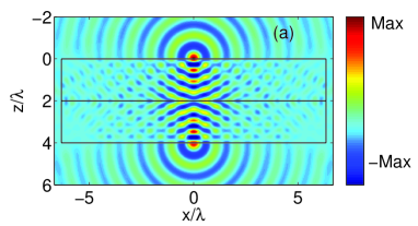
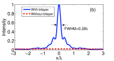
Figure 3: (a) Electric field distribution for a line current source $J_{s}=A\delta(z+0.01\lambda)\delta(x)$ interacting with a bilayer lens located in $z\in[0,4\lambda]$; (b) Field intensities at the exit boundary $z=4\lambda$ for the cases with the bilayer and without bilayer. The bilayer lens has $\epsilon_{1}=4$, $\mu_{1}=1$, $\epsilon_{2}=-4+0.008i$ and $\mu_{2}=-1+0.008i$ and $L_{1}=L_{2}=2\lambda$.

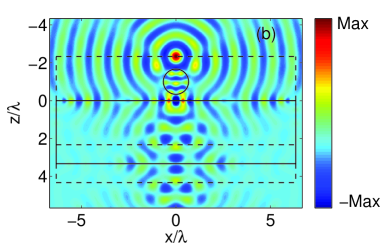
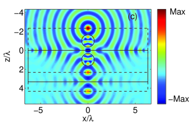
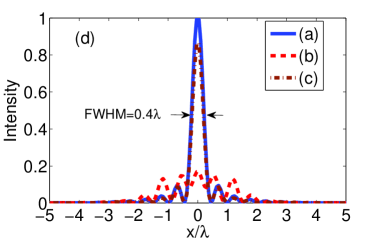
Figure 4: (a) Electric field distribution for a line current source $J_{s}=A\delta(z+7/3\lambda)\delta(x)$ interacting with a Pendry’s lens $\epsilon_{L}=-1+0.008i$ and $\mu_{l}=-1+0.008i$; (b) electric field distribution when a dielectric cylinder is put in the front of the lens; (c) electric field distribution when the dielectric cylinder together with its compensated cylinder are put outside and inside the lens, respectively. (d) Field intensity at the image plane $z=13/3\lambda$ for (a), (b) and (c). The dielectric cylinder has a radius of $2/3\lambda$ with the center at $z=-\lambda$ and $x=0$, and a refractive index of $2$.

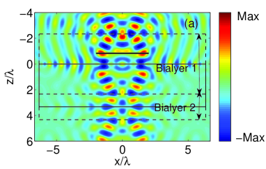
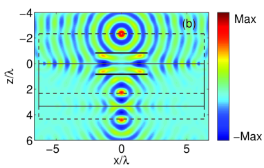
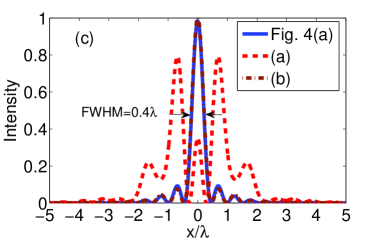
Figure 6: Electric field distribution when (a) a current sheet $J_{s}=4A\delta(x+z/6\lambda)\;x\in[-2\lambda,2\lambda]$ is put in the front of the lens of Fig. 4(a); (b) the compensated current sheet is put inside the lens. (c) Field intensity at the the image plane $z=13/3\lambda$ for (a), (b), and also Fig. 4(a).

References

- (1) J. B. Pendry, D. Schurig, and D. R. Smith, Science 312, 1780 (2006).
- (2) U. Leonhardt, and T. G. Philbin 2008 http: //www.arXiv:0805.4778v2 [physics.optics].
- (3) U. Leonhardt, Science 312, 1777 (2006).
- (4) D. Schurig, J. J. Mock, B. J. Justice, S. A. Cummer, J. B. Pendry, A. F. Starr, and D. R. Smith, Science 314, 977 (2006).
- (5) W. Cai, U. K. Chettiar, A. V. Kildishev, V. M. Shalaev, Nat. Photonics 1, 224-227 (2007).
- (6) S. A. Cummer, B. I. Popa, D. Schurig, D. R. Smith, and J. B. Pendry, Phys. Rev. E. 74, 036621 (2006).
- (7) Z. C. Ruan, M. Yan, C. W. Neff, and M. Qiu, Phys. Rev. Lett. 99, 113903 (2007).
- (8) H. S. Chen, B. I. Wu, B. L. Zhang, and J. A. Kong, Phys. Rev. Lett. 99, 063903(2007).
- (9) U. Leonhardt, New J. Phys. 8, 247 (2006).
- (10) M. Yan, Z. C. Ruan, and M. Qiu, Phy Rev. Lett. 99, 233901(2007).
- (11) M. Rahm, S. A. Cummer, D. Schurig, J. B. Pendry, and D. R. Smith, Phys. Rev. Lett. 100, 063903 (2008).
- (12) H. Y. Chen and C. T. Chan, Appl. Phys. Lett. 90, 241105 (2007).
- (13) A. Greenleaf, Y. Kurylev, M. Lassas, and G. Uhlmann, Phys. Rev. Lett. 99, 183901 (2007).
- (14) J. B. Pendry, Phys. Rev. Lett. 85, 3966-3969 (2000).
- (15) M. Yan, W. Yan, and M. Qiu, Phys. Rev. B 78, 125113 (2008).
- (16) J.B. Pendry, and S.A. Ramakrishna, J. Phys. Condensed Matter. 14, 6345 (2003).
- (17) D.R. Smith, and S. Schurig, Phys. Rev. Lett. 90, 077405 (2003).
- (18) D Schurig and D R Smith, New Journal of Physics 7, 162 (2005).