Abstract

Data on $K_{e4}$ decays allow one to extract experimental information on the elastic $\pi\pi$ scattering amplitude near threshold, and to confront the outcome of the analysis with predictions made in the framework of QCD. These predictions concern an isospin symmetric world, while experiments are carried out in the real world, where isospin breaking effects – generated by electromagnetic interactions and by the mass difference of the up and down quarks – are always present. We discuss the corrections required to account for these, so that a meaningful comparison with the predictions becomes possible. In particular, we note that there is a spectacular isospin breaking effect in $K_{e4}$ decays. Once it is taken into account, the previous discrepancy between NA48/2 data on $K_{e4}$ decays and the prediction of $\pi\pi$ scattering lengths disappears.

Pacs:	11.30.Rd, 12.38.Aw, 13.20.-v, 12.39.Fe
Keywords:	$K_{e4}$ decays, isospin breaking, pion-pion scattering,
	chiral symmetries

1 Introduction

Chiral perturbation theory (ChPT) [1], combined with Roy equations, allows one to make very precise predictions for the values of the threshold parameters in elastic $\pi\pi$ scattering [2] – for a status report, see e.g. the contribution of one of us at KAON’07 [3]. Several experiments have measured the $\pi\pi$ interaction at low energy with a precision such that it is now possible to confront these predictions with data: i) $K^{+}\to\pi^{+}\pi^{-}e^{+}\nu_{e}$ decays [4, 5, 6, 7, 8], ii) the pionium lifetime, measured by the DIRAC collaboration [9], iii) the cusp effect in $K\to 3\pi$ decays, investigated by the NA48/2 and KTeV collaborations [10, 8]. The experiments performed by the NA48/2 collaboration have generated an impressive data basis, as a result of which the matrix elements of $K\to 3\pi$ and of $K_{e4}$ decays can be determined with an unprecedented accuracy.

The theoretical predictions and the measurements are performed in two different settings: the predictions concern pure QCD, in the isospin symmetry limit $m_{u}=m_{d}$, with photons absent – a paradise world. To be more precise, the convention is to choose the quark masses and the renormalization group invariant scale of QCD such that the pion and the kaon masses coincide with the values of the charged ones, and the pion decay constant is $F_{\pi}=92.4$ MeV. [We do not specify the masses of the heavy quarks, because in the present context, their precise values do not matter.] On the other hand, experiments are all carried out in the presence of isospin breaking effects, generated by real and virtual photons, and by the mass difference of the up and down quarks: this is the real world, described by the Standard Model. We are thus faced with the problem to find the relation between quantities measured in the real world, where isospin breaking effects are always present, and the predictions made in the paradise world. It is the aim of the present article to provide this relation.

In early experiments [4], the effects of real and virtual photons were estimated by considering a simplified model for the weak interactions, and taking into account photon effects through minimal coupling, working at lowest nontrivial order in $\alpha_{\mathrm{QED}}$. In analyses of NA48/2 data before spring 2007, real and virtual photon effects were treated in a factorized manner, applying the Coulomb factor and using the program PHOTOS [11] – see Ref. [5] for details. It is clear that both approaches missed the effects generated by the pion and kaon mass differences, and by the quark mass difference $m_{d}-m_{u}$. It turned out that these effects are quite spectacular [12, 13, 14, 15]: when taken into account, all previous discrepancies between data and prediction for the scattering lengths disappear [3, 6, 7, 8].

The outline of the paper is as follows. In section 2, we recall how $K_{e4}$ data are analysed in the isospin symmetry limit, based on Watson’s theorem, while section 3 describes the framework in which we take isospin breaking effects into account. In section 4 we investigate – for the case of (Lorentz) scalar pion form factors – the effect of isospin breaking mass differences using unitarity and analyticity alone. We illustrate the outcome of this investigation in section 5 with two explicit examples in the framework of Quantum Field Theory, before we return to $K_{e4}$ decays in section 6, where we display the result for the changes in the phase of the form factors, and for the phase–removed form factors themselves. These results allow us in section 7 to perform fits to $K_{e4}$ data, based on numerical solutions to Roy equations, and to determine in this manner experimental values for the $\pi\pi$ scattering lengths. A comparison with related work available in the literature is provided in the following section 8, while a summary and concluding remarks are given in section 9. Appendix B contains proofs of the general statements made on the low–energy structure of phases and form factors in the main text. Finally, Appendix C contains material needed for the calculations of form factors in a non-relativistic framework.

2 $K_{e4}$ decays: isospin symmetry limit

To set notation and to explain the manner in which $K_{e4}$ decays allow one to measure $\pi\pi$ phase shifts, let us consider here the decays in the isospin symmetry limit $m_{u}=m_{d},\alpha_{\mathrm{QED}}$ =0. The matrix element for $K^{+}(p)\to\pi^{+}(p_{1})\pi^{-}(p_{2})e^{+}(p_{e})\nu_{e}(p_{\nu})$ is

$$T=\frac{G_{F}}{\sqrt{2}}V^{\star}_{us}\bar{u}(p_{\nu})\gamma^{\mu}(1-\gamma_{5})v(p_{e})(V_{\mu}-A_{\mu}),$$ (1)

where the last factor denotes hadronic matrix elements of the strangeness changing (vector and axial vector) currents,

$$V_{\mu}-A_{\mu} = \langle\pi^{+}(p_{1})\pi^{-}(p_{2})\,\mbox{out}\mid(\bar{s}\gamma_{\mu}u-\bar{s}\gamma_{\mu}\gamma_{5}u)\mid K^{+}(p)\rangle\,.$$ (2)

In the following, we concentrate on the matrix element of the axial vector current, because it carries information on the $\pi\pi$ final state interactions and, in particular, on the $\pi\pi$ phase shifts. One decomposes $A_{\mu}$ into Lorentz scalars,

$$A_{\mu}=-i\frac{1}{M_{K}}\left[(p_{1}+p_{2})_{\mu}F+(p_{1}-p_{2})_{\mu}G+(p_{e}+p_{\nu})_{\mu}R\right]\,.$$ (3)

The form factors $F,G,R$ are holomorphic functions of the three variables

$$s=(p_{1}+p_{2})^{2}\,,\,t=(p_{1}-p)^{2}\,,\,u=(p_{2}-p)^{2}\,\,.$$ (4)

Sometimes, it is useful to use instead

$$s=(p_{1}+p_{2})^{2}\,,\,s_{\ell}=(p_{e}+p_{\nu})^{2}\,,\,\cos{\theta_{\pi}}\,,\,$$ (5)

where $\theta_{\pi}$ is the angle of the $\pi^{+}$ in the CM system of the two charged pions, with respect to the dipion line of flight in the rest system of the kaon [17]. In the isospin symmetry limit, one identifies the $\pi\pi$ phase shifts in the matrix element in a standard manner, by performing a partial wave expansion, and using unitarity and analyticity, although, in the present case, this is a slightly intricate endeavour [18]. It is useful to introduce a particular combination of form factors (we omit isospin indices),

$$F_{1}=F+\frac{(M_{K}^{2}-s-s_{\ell})\sigma}{\lambda(M_{K}^{2},s,s_{\ell})^{1/2}}\cos{\theta_{\pi}}G\,.$$ (6)

Here, $\sigma=\sqrt{1-4M_{\pi}^{2}/s}$, and $\lambda(x,y,z)$ is the triangle function. The form factor $F_{1}$ has a simple partial wave expansion,

$$F_{1}=\sum_{k\geq 0}P_{k}(\cos{\theta_{\pi}})f_{k}(s,s_{\ell})\,.$$ (7)

For fixed $s_{\ell}$, the amplitudes $f_{k}$ are holomorphic in $\mathbb{C}_{LR}(4M_{\pi}^{2})$. In the elastic region, the form factors $f_{k}$ carry the $\pi\pi$ phase shifts in the pertinent isospin channel [18]. For $f_{0}$ and $f_{1}$, the relation is

$$f_{0}^{+} = e^{2i\delta_{0}}f_{0}^{-}\,,\,f_{1}^{+}=e^{2i\delta_{1}}f_{1}^{-}\,;\quad s\in[4M_{\pi}^{2},16M_{\pi}^{2}]\,,\,$$ (8)

where $\delta_{0}$ ($\delta_{1}$) denotes the phase shift of the isospin zero S-wave (isospin one P-wave), and $f_{n}^{+}(f_{n}^{-})$ stands for the form factor evaluated above (below) the cut,

$$f_{n}^{\pm} = f_{n}(s\pm i\epsilon,s_{\ell})\,.$$ (9)

The phase–removed form factor can be Taylor expanded at threshold. For the quantity $f_{0}$, the expansion reads

$$e^{-i\delta_{0}}f^{+}_{0}=c_{0}+c_{2}q^{2}+O(q^{4})\,,\,\quad q^{2}=\frac{s}{4M_{\pi}^{2}}-1\,,\,$$ (10)

with coefficients $c_{i}$ that depend on $s_{\ell}$. Because the modulus squared $|F_{1}|^{2}$ enters the decay rate, one can measure the phase shift difference $\delta_{0}-\delta_{1}$ in $K_{e4}$ decay experiments. In the remaining part of this article, we investigate the manner in which the relations Eqs. (8,10) are modified in the presence of isospin symmetry breaking effects, and how the analysis of $K_{e4}$ data must be modified in order to determine the $\pi\pi$ phase shifts.

Figure 1: Some of the graphs that contribute to the matrix element of the axial current at tree and one–loop order. The filled vertex indicates that the axial current also couples to a single kaon line. That graph contributes to the form factor $R$. There are many additional graphs at one–loop order, not displayed in the figure.

Before proceeding, let us consider the form factors at one loop in chiral perturbation theory and verify that $F_{1}$ indeed has the behaviour just discussed. For this, we recall the pertinent effective Lagrangian

$${\cal L}_{2}=\frac{F_{0}^{2}}{4}\langle D_{\mu}UD^{\mu}U^{\dagger}+2B_{0}{\cal M}(U+U^{\dagger})\rangle\,,$$ (11)

where the covariant derivative $D_{\mu}U$ contains the external vector and axial vector currents, and ${\cal M}=\mathrm{diag}(\hat{m},\hat{m},m_{s})$. Some of the graphs that contribute at tree–level and at one loop are displayed in figure 1. The full result is [19]

$$f_{0}(s,s_{\ell})=\frac{M_{K}}{\sqrt{2}F_{0}}\left\{1+\Delta(s)+H(s,s_{\ell})+O(p^{4})\right\}\,,$$ (12)

with

$$\Delta(s) = \frac{1}{2F_{0}^{2}}(2s-M_{\pi}^{2}){\bar{J}}(s)\,,$$

$$16\pi^{2}\bar{J}(s) = \sigma\left(\ln{\frac{1-\sigma}{1+\sigma}}+i\pi\right)+2\,,\quad s\geq 4M_{\pi}^{2}\,.$$ (13)

Here, $M_{\pi}$ ($F_{0}$) denotes the pion mass (pion decay constant), at leading order in the chiral expansion. The quantity $H(s,s_{\ell})$ is real in the interval of elastic $\pi\pi$ scattering. It is now seen that $f_{0}$ indeed has the property (8) at this order in the low–energy expansion, with

$$\delta_{0}=\frac{(2s-M_{\pi}^{2})}{32\pi F_{0}^{2}}\sigma\,.$$ (14)

This is the phase shift of the isospin zero S-wave, in tree approximation. The amplitude $f_{1}$ has a very similar structure [19], containing the phase shift of the isospin one P-wave, again in tree approximation. Remark: To get the result Eq. (14), we have used an expansion around the chiral limit $m_{u}=m_{d}=m_{s}=0$, as a result of which the pertinent pion decay constant $F_{0}$ in this limit appears. To the order considered here, we may replace $F_{0}$ by the pion decay constant $F$ in the chiral limit $m_{u}=m_{d}=0,m_{s}\neq 0$. It seems to us that this is a more natural choice when discussing the $\pi\pi$ phase shift, and we will, therefore, use $F_{0}\Rightarrow F$ in numerical analyses in the rest of this article.

3 Isospin breaking: the framework

The relation (8) holds in the isospin symmetry limit. On the other hand, $K_{e4}$ decays happen to occur in the real world where $m_{d}\neq m_{u},\alpha_{\mathrm{QED}}\neq 0$, as a result of which the relations Eq. (8) do not hold anymore. Here, we discuss how this situation can be modelled in view of the already published analyses of $K_{e4}$ decays.

In early experiments [4], the effects of real and virtual photons were estimated by considering a simplified model for the weak interactions, and taking into account photon effects through minimal coupling, working at lowest nontrivial order in $\alpha_{\mathrm{QED}}$. In analyses of NA48/2 data before summer 2007, real and virtual photon effects were treated in a factorized manner, applying the Coulomb factor and using the program PHOTOS [11] – see Ref. [5] for details. It is clear that both approaches missed the effects generated by the pion and kaon mass differences, and by the quark mass difference $m_{d}-m_{u}$. These must thus be taken into account separately. We assume that they can be evaluated in factorized form as well, and write symbolically in case of the NA48/2 analysis

Full isospin breaking effects = Coulomb factor $\times$ PHOTOS $\times$ mass effects

As a practical way of proceeding, which should catch the main effects, we propose to correct also earlier analyses [4] with the last factor.

We now discuss the manner in which mass effects may be evaluated. As the correction turns out to be small (although not negligible), a perturbative method is appropriate. In the following, we use effective field theory techniques to perform the calculation. As real and virtual photons have already been taken into account, we need a framework that accounts for mass effects only. An obvious candidate is the chiral lagrangian itself, in the absence of real photons. This can be achieved by modifying the lagrangian ${\cal L}_{2}$: one adapts the quark mass matrix, ${\cal M}\to\mathrm{diag}(m_{u},m_{d},m_{s})$, and adds mass breaking terms of electromagnetic origin [20],

$${\cal L}_{2}\to{\cal L}_{2}+C\langle QUQU^{\dagger}\rangle\,,\qquad Q=\frac{e}{3}\mathrm{diag}(2,-1,-1)\,,$$ (15)

where $C$ is a low–energy constant that breaks the isospin symmetry of the meson masses, such that $M_{\pi}\neq M_{\pi^{0}},M_{K}\neq M_{K^{0}}$. The symbol $e$ stands for the electric charge. At order $p^{4}$, there will be additional terms, classified in Refs. [21, 20]. The effect of the replacement (15) is twofold: first, because the pion masses split, the loop contributions generated by the diagrams displayed in Fig. 1b),c) have a different threshold. Second, in addition to the graphs displayed in figure 1, there is a new contribution shown in figure 2: the kaon interacts with the axial current to generate a $\pi^{0}\eta$ intermediate state. Because $m_{u}\neq m_{d}$, the $\eta$ can transform back into a neutral pion, that then re–scatters with the second neutral pion into a charged pion pair. We perform later in this article a quantitative analysis of these effects.

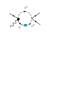
Figure 2: One–loop graph in the $K_{e4}$ decay amplitude that emerges due to the $\pi^{0}\eta$ mixing. There is no counterpart of this graph in the scalar form factor.

In summary, we propose the following framework to purify published phase shifts from mass effects.

• We assume that the published phase shifts correspond to the ones obtained in a world defined by the lagrangian (15),

  $$f_{k}^{+}=e^{2i\psi_{k}}f_{k}^{-}\,,\,k=0,1\,;\,s\geq 4M_{\pi}^{2}\,.$$ (16)

  We refer in the following to $\psi_{k}$ as “measured phase shifts”.

• In order to get into contact with the isospin symmetric phase shifts $\delta_{k}$, we note that

  $$\delta_{k} = \psi_{k}-(\psi_{k}-\delta_{k})\,,\,k=0,1\,.$$ (17)

  The differences $\psi_{k}-\delta_{k}$ on the right–hand side are small, and can be calculated in the effective field theory framework outlined above. After subtracting these from the measured phase shifts $\psi_{k}$, one gets $\delta_{k}$, which can then be confronted with predictions in the framework of ChPT.

While this procedure does not present a complete and full analysis of radiative corrections in $K_{e4}$ decays, it allows one to purify published phase shifts from mass effects and thus to hopefully retain the main effects of isospin breaking. [One may envisage a more ambitious procedure [22], by working out the relevant matrix elements in the framework of ChPT including photons and leptons [23], and then constructing a new event generator, to be used in a new analysis of $K_{e4}$ decays. Eventually, such an analysis might lead to an improved algorithm. However, we consider this to be a long term project.]

The framework proposed here allows one to investigate the strictures imposed on the form factors by unitarity and analyticity, even without relying on any specific details of the lagrangian Eq. (15). We find it instructive to discuss this fact in some detail in the following section – before performing the explicit evaluation of isospin breaking effects in $K_{e4}$ decays – because it illustrates that, qualitatively, the effects we are finding at the end in those decays do not rely on a specific lagrangian framework, but are present in any theory that breaks isospin symmetry and incorporates unitarity and analyticity. [On the other hand, to work out the effects in a quantitative manner, a specific underlying theory is needed.] Readers who are not interested in this general setting may wish to skip the following two sections and continue directly with section 6, where we take up the case of $K_{e4}$ decays again, and where we calculate the corrections $\psi_{0}-\delta_{0}$ and $\psi_{1}-\delta_{1}$, and investigate their effect on the $\pi\pi$ scattering lengths.

4 Watson’s theorem and all that

Here, we discuss Watson’s theorem and its modification in the isospin breaking case by using analyticity and unitarity arguments alone. As already mentioned, it is not quite straightforward to work out unitarity and analyticity constraints on the axial current matrix element Eq. (3) which is relevant here, because this matrix element describes the scattering process $K+\mbox{axial current}\to\pi+\pi$, which has a rather complicated structure. On the other hand, the physical effects generated by isospin breaking interactions are also present in simpler matrix elements like the (Lorentz) scalar form factor of the pion. We, therefore, illustrate the basic facts in this simpler setting. It will become obvious that the same line of reasoning could be carried over in the same general framework to the $K_{e4}$ form factors, although with much more labor.

To set the framework, we consider matrix elements of a hermitian Lorentz scalar current $j(x)$, which is taken to be isoscalar in the absence of isospin breaking interactions. To simplify the analysis further, we consider the case where the isospin symmetric theory corresponds to the standard $SU(2)_{R}\times SU(2)_{L}\to SU(2)$ scenario of spontaneously broken two-flavour QCD, with pions only. Emission of real photons is excluded, as a result of which all matrix elements are infrared finite.

As isospin symmetry is assumed to be broken, it is convenient to use state vectors that are labelled by the physical pion states. The two form factors are

$$\langle 0|j(0)|\pi^{+}(p_{1})\pi^{-}(p_{2});\mbox{in}\rangle = -F_{c}(s)\,,$$

$$\langle 0|j(0)|\pi^{0}(p_{1})\pi^{0}(p_{2});\mbox{in}\rangle = F_{0}(s)\,,\quad\quad s=(p_{1}+p_{2})^{2}\,.$$ (18)

In the isospin symmetry limit, one has $F_{c}=F_{0}$ in the Condon-Shortley phase convention used here. These form factors are boundary values of functions $F_{k}(z)$ which are assumed to be i) holomorphic in $\mathbb{C}_{R}(4M_{\pi^{0}}^{2})$, and ii) real on the real axis for $s<4M_{\pi^{0}}^{2}$. For further specifications of $F_{k}$ needed to arrive at the results described below, see Appendix B.

We also need the elastic $\pi\pi\to\pi\pi$ scattering matrix elements and consider the following three channels in $\pi^{a}\pi^{b}\to\pi^{c}\pi^{d}:(ab;cd)=(00;00),(+-;00),(+-;+-)$. We denote the scattering matrix elements by $T_{i}(s,t)$, where $i=0,x,c$ are the channel labels in the above order, and $s,t$ stand for the Mandelstam variables. The partial-wave expansion reads

$$T_{i}(s,t)=32\pi\left[h_{i}(s)+\sum_{l=1}^{\infty}P_{l}(\cos\vartheta)h^{l}_{i}(s)\right]\,,$$ (19)

Here, $\vartheta$ stands for the scattering angle, and $h_{i}(s)$ denote the pertinent S-waves, which are needed in the following. They are boundary values of functions $h_{i}(z)$ which are assumed to be i) holomorphic in $\mathbb{C}_{LR}(4M_{\pi^{0}}^{2})$, and ii) real on the real axis for $0<s<4M_{\pi^{0}}^{2}$. For further specifications of $h_{k}$ needed to arrive at the results described below, see Appendix B.

The unitarity conditions for the form factors and for the partial waves read on the upper rim of the cut

$${\rm Im}\,F(s) = T(s)\rho(s)F^{*}(s)\,,\,$$

$${\rm Im}\,T(s) = T(s)\rho(s)T^{*}(s)\,;\,\quad 4M_{\pi^{0}}^{2}\leq s\leq 16M_{\pi^{0}}^{2}\,.$$ (20)

We have used the matrix notation

$$F=\left(\!\!\begin{array}[]{c}F_{c}\\ F_{0}\end{array}\!\!\right)\,,\,\quad\quad T=\left(\!\!\begin{array}[]{rr}h_{c}&-h_{x}\\ -h_{x}&h_{0}\end{array}\!\!\right)\,,\,$$ (25)

$$\rho(s)=\left(\!\!\begin{array}[]{cc}2\sigma(s)\,\theta(s-4M_{\pi}^{2})&0\\ 0&\sigma_{0}(s)\,\theta(s-4M_{\pi^{0}}^{2})\end{array}\!\!\right)\,,\,$$ (28)

together with

$$\sigma(s)=\sqrt{1-\frac{4M_{\pi}^{2}}{s}}\quad,\quad\sigma_{0}(s)=\sqrt{1-\frac{4M_{\pi^{0}}^{2}}{s}}\,.$$ (29)

The quantity $\sigma(z)$ is holomorphic in $\mathbb{C}_{LR}(4M_{\pi}^{2})$. On the upper rim of the right–hand cut we take $\sigma(z)$ to be positive and real, and the analytic continuation thereof elsewhere in the complex $z$-plane. Analogous statements hold for $\sigma_{0}(z)$.

4.1 Isospin symmetry limit

In the isospin symmetry limit, one has

$$\left(h_{c}\,,\,h_{x}\,,\,h_{0}\right)=\frac{1}{6}\left(t_{2}+2t_{0}\,,\,2t_{2}-2t_{0}\,,\,4t_{2}+2t_{0}\right)\,.$$ (30)

The quantity $t_{I}$ denotes the partial wave amplitude with angular momentum zero and isospin $I$. With $F_{c}=F_{0}$, the unitarity relations Eq. (4) decouple,

$${\rm Im}F_{c} = t_{0}\sigma F^{*}_{c}\,,\,$$

$${\rm Im}\,t_{I} = \sigma|t_{I}|^{2}\,,\,I=0,2\,.$$ (31)

We analyse in Appendix B the singularity structure of the partial waves and of the form factor which follow from these relations [24]. The result is as follows:

• The form factor develops a square root singularity at the threshold $z=4M_{\pi}^{2}$,

  $$F_{c}(z)=A(z)+i\sigma B(z)\,,\,$$ (32)

  where $A,B$ are meromorphic in $\mathbb{C}_{LR}(16M_{\pi}^{2})$, and real on the real axis in the interval $0<s<16M_{\pi}^{2}$.

• Define the phase

  $${\theta(z)} = \arctan{\frac{\sigma(z)B(z)}{A(z)}}\,.$$ (33)

  In the elastic interval, $\theta$ coincides with the phase shift $\delta_{0}$ of the partial wave $t_{0}$ – this is Watson’s theorem. The above definition of $\theta$ holds also for complex values of $z$. As a result, $\theta$ is holomorphic in the shaded region shown in Fig. 3, cut along the positive real axis for $s>4M_{\pi}^{2}$. [Although $\theta(z)$ is complex in general, we keep calling this quantity phase for simplicity.]

• In analogy to Eq. (10), we define the phase–removed form factor

  $$\hat{F}_{c}(z) = e^{-i\theta(z)}F_{c}(z)=A\left(1+\frac{\sigma^{2}B^{2}}{A^{2}}\right)^{1/2}\,.$$ (34)

  $\hat{F}_{c}$ is holomorphic in the shaded region shown in figure 3, and real on the real axis in that region. It can therefore be Taylor expanded at threshold,

  $$\hat{F}_{c}=\sum_{i\geq 0}e_{i}(z-4M_{\pi}^{2})^{i}\,,\,$$ (35)

  with real coefficients $e_{i}$, cf. with Eq. (10).

Analogous facts were (implicitly and explicitly) used for the axial form factors $f_{k}$ in Eq. (7) in all previous analyses of $K_{e4}$ decays.

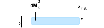
Figure 3: Region of analyticity in the complex $z$-plane, isospin symmetric case. The phase–removed form factor $\hat{F}_{c}(z)$ is holomorphic in the shaded region. The symbol $z_{inel.}$ denotes the inelastic threshold $z=16M_{\pi}^{2}$.

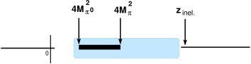
Figure 4: Region of analyticity, isospin broken case. The phase–removed form factors $\hat{F}_{k}$ are holomorphic in the (cut) shaded region. The symbol $z_{inel.}$ denotes the inelastic threshold $z=16M_{\pi^{0}}^{2}$.

4.2 Broken isospin symmetry

We now consider the case where the underlying theory contains isospin breaking interactions. To render the discussion simple, we assume that these terms are reasonably small, such that the isospin symmetric values of the form factors and of the scattering matrix are only slightly modified. This can always be arranged by adjusting the relevant parameters in the lagrangian, and allows us to discuss the changes induced in a simpler manner. We analyse the singularity structure of the form factors $F_{c,0}$ in Eq. (4) in the general case in Appendix B as well, and we find that the four statements i) to iv) made above are modified in the following manner:

• The form factors have the threshold behaviour

  $$F_{k}=A_{k}+i\sigma B_{k}+i\sigma_{0}C_{k}+\sigma\sigma_{0}D_{k}\,;\,k=c,0\,,\,$$ (36)

  with coefficients $A_{k},\ldots,D_{k}$ that are meromorphic in $\mathbb{C}_{LR}(16M_{\pi^{0}}^{2})$, and real on the real axis in the interval $0<s<16M_{\pi^{0}}^{2}$.

• Let

  $${\theta_{k}(z)} = \arctan{\frac{\sigma(z)B_{k}(z)+\sigma_{0}(z)C_{k}(z)}{A_{k}(z)+\sigma(z)\sigma_{0}(z)D_{k}(z)}}\,,$$ (37)

  and introduce the phase–removed form factors $\hat{F}_{k}$,

  $$\hat{F}_{k}(z) = e^{-i\theta_{k}(z)}F_{k}(z)\,.$$ (38)

  The quantities $\hat{F}_{k}$ are holomorphic in the (cut) shaded region shown in Fig. 4, and real on the real axis in the intervals $0<s<4M_{\pi^{0}}^{2}$ and $4M_{\pi}^{2}<s<16M_{\pi^{0}}^{2}$.

• In contrast to the isospin symmetric case one finds that

  • the $\pi\pi$ scattering amplitude does not fully determine the phases $\theta_{k}$ below the inelastic region,

  • $\theta_{c}$ does not vanish at the threshold $s=4M_{\pi}^{2}\,,\,$

    $$\theta_{c}\not\to 0\,,\,s\to 4M_{\pi}^{2}\,.$$ (39)

• Again in contrast to the isospin symmetric case, the form factor $\hat{F}_{c}$ develops a square root singularity at $z=4M_{\pi}^{2}$,

  $$\hat{F}_{c}(s)=\bar{e}_{0}+\bar{e}_{1}q+O(q^{2})\,,\,s\searrow 4M_{\pi}^{2}\,;\,$$ (40)

  with real coefficients $\bar{e}_{i}$ .

This result shows that the phase–removed form factor $\hat{F}_{c}$ cannot be expanded in a Taylor series at the threshold $s=4M_{\pi}^{2}$. [One may be tempted to get rid of the problem by defining a form factor where the pertinent Omnès factor is removed. In the present case, this is not what one wants to do, because the aim is to measure the phase shift, which is needed to evaluate the Omnès factor.]

5 Explicit examples

We find it useful to provide in this section examples of form factors that illustrate the analytic properties worked out above.

5.1 Scalar form factor in a non-relativistic effective theory

In order to describe the behaviour of the scalar form factor in the low–energy region $q^{2}=s/(4M_{\pi}^{2})-1\ll 1,~{}\Delta_{\pi}=M_{\pi}^{2}-M_{\pi^{0}}^{2}\ll M_{\pi}^{2}$, we use the framework of non-relativistic effective field theory (NREFT) as developed in Refs. [25, 26, 27, 28]. This formulation is especially convenient to study the singularity structure near threshold, because the locations of the low–energy singularities coincide with that in the relativistic QFT to all orders in the low–energy expansion. A similar non-relativistic framework has recently been used to study $K\to 3\pi$ decays in the vicinity of cusps [25, 26, 27]. The effects that we are addressing in this section have the same physical origin as the cusps in $K\to 3\pi$ decays. They emerge, because the final state interactions involve both, $\pi^{+}\pi^{-}$ and $\pi^{0}\pi^{0}$ pairs, with different masses $M_{\pi}\neq M_{\pi^{0}}$. We display the pertinent non-relativistic lagrangian in Appendix C.

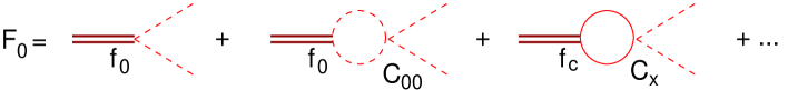
Figure 5: Bubble diagrams, contributing to the neutral scalar form factor in the non-relativistic effective theory. Solid and dashed lines correspond to charged and neutral pions, respectively.

The scalar form factors $F_{c}(s)$ and $F_{0}(s)$, defined in Eq. (C), are given by a sum of bubble diagrams, see Fig. 5. The infinite series of these bubble diagrams can be explicitly re-summed. The resulting expressions for $F_{c}(s)$, $F_{0}(s)$ are boundary values of meromorphic functions $F_{c}(z)$, $F_{0}(z)$ at $z\to s+i0$, with

$$F_{c}(z) = \frac{f_{c}(1-2i\sigma_{0}d_{0})-2i\sigma_{0}f_{0}d_{x}}{1-2i\sigma_{0}d_{0}-4i\sigma d_{c}-2\sigma\sigma_{0}\chi}\,,$$

$$F_{0}(z) = \frac{-4i\sigma f_{c}d_{x}+f_{0}(1-4i\sigma d_{c})}{1-2i\sigma_{0}d_{0}-4i\sigma d_{c}-2\sigma\sigma_{0}\chi}\,,$$ (41)

where $d_{i},~{}i=c,x,0$ and $f_{k},~{}k=c,0$ denote polynomials of first order in $z$, and $\chi=4(d_{c}d_{0}-d_{x}^{2})$. The coefficients of these polynomials are expressed through various non-relativistic couplings which, in turn, are determined by performing the matching to the underlying relativistic theory (see, e.g. [25, 26, 27, 28]). In particular, the polynomials $d_{i}$ contain 4-pion non-relativistic couplings and are expressed in terms of the effective-range expansion parameters for the $\pi\pi$ scattering through the matching of the $\pi\pi$ amplitudes at threshold. Similarly, the polynomials $f_{k}$ are determined from the matching to the relativistic form factors, expanded at threshold.

Further, the quantities $d_{i},f_{k}$ contain isospin-breaking corrections. We write $d_{i}=\bar{d}_{i}+d_{i}^{\prime}$ (and similarly for $f_{k}$), where $\bar{d}_{i}$ stands for $d_{i}$ calculated in the isospin limit. In analogy with Eq. (30), $\bar{d}_{i}$ can be expressed through two first-order polynomials $v_{0},v_{2}$, corresponding to total isospin $I=0,2\,,\,$

$$(\bar{d}_{c},\,\bar{d}_{x},\,\bar{d}_{0})=\frac{1}{12}\,(v_{2}+2v_{0},\,2v_{2}-2v_{0},\,4v_{2}+2v_{0})\,.$$ (42)

Here,

$$v_{I}(z)=a_{I}+\frac{z-4M_{\pi}^{2}}{4M_{\pi}^{2}}\,a_{I}r_{I}\,,\quad\quad I=0,2\,,$$ (43)

and $a_{I}$/$a_{I}r_{I}$ stand for the scattering length/effective range parameter in the isospin limit, see Ref. [25].

Providing similar explicit expressions for the isospin-breaking corrections in $d_{i}$ and $f_{k}$ is not possible in general. The form of these corrections is not universal and the calculations should be performed within a particular underlying relativistic theory. An example of calculations in ChPT at one loop is considered in the following subsection.

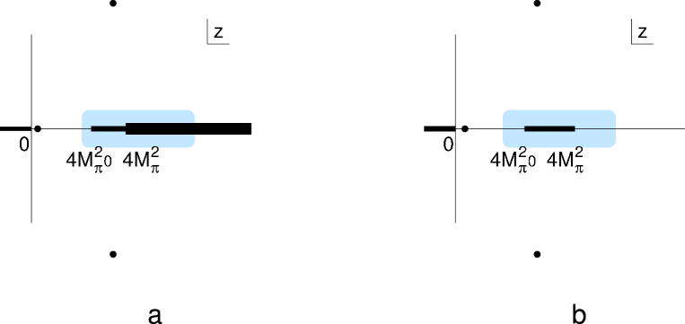
Figure 6: The analyticity domain of the form factor $F_{c}(z)$ (left panel) and the phase–removed form factor $\hat{F}_{c}(z)$ (right panel). The shaded area denotes the non-relativistic region and the filled circles indicate the positions of the poles on the first Riemann sheet. Both the left-hand cut and the poles lie outside the non-relativistic domain.

We add several comments concerning the structure of the two form factors.

• As already mentioned, the form factors $F_{c}(z)$, $F_{0}(z)$ are meromorphic functions in the cut plane displayed in Fig. 6a. The non-relativistic domain in the complex plane is defined as a strip surrounding the physical cut – it is indicated with the shaded region in the figure. It extends slightly below and above of the physical branch point, well below the first inelastic threshold. The maximal distance to the branch point in the non-relativistic region is set by the mass scale $M_{\pi}$. NREFT makes sense only in the non-relativistic region – the cut along the negative $z$-axis, as well as the distant poles on the first sheet should be regarded as artefacts of the non-relativistic treatment.

• The form factors have the representation (36). Constructing the $\pi\pi$ amplitudes in the same manner as the form factors, one finds that the unitarity relation given in Eq. (4) indeed is satisfied.

• In order to obtain the phase–removed form factor, we define the phase as in Eq. (37),

  $$\theta_{c}(z) = \arctan\frac{P-Q}{1+PQ}\,,$$

  $$P = \frac{2\sigma_{0}d_{0}+4\sigma d_{c}}{1-2\sigma\sigma_{0}\chi}\,,\quad\quad Q=2\sigma_{0}\biggl{(}d_{0}+\frac{f_{0}}{f_{c}}\,d_{x}\biggr{)}\,.$$ (44)

  The phase–removed form factor

  $$\hat{F}_{c}(z)=\frac{f_{c}}{1-2\sigma\sigma_{0}\chi}\,\biggl{(}\frac{1+Q^{2}}{1+P^{2}}\biggr{)}^{1/2}$$ (45)

  is holomorphic in the (cut) shaded region shown in Fig. 6b. This differs from the isospin symmetric case, where the cut from $4M_{\pi^{0}}^{2}$ to $4M_{\pi}^{2}$ is absent.

  In conformity with Eq. (40), the expansion of $\hat{F}_{c}(z)$ at threshold contains even and odd powers of the variable $q$,

  $$\hat{F}_{c}(z) = \hat{F}_{c}(4M_{\pi}^{2})(1+\bar{e}_{1}q+\bar{e}_{2}q^{2}+O(q^{3}))\,,\,s\!\!\searrow 4M_{\pi}^{2}\,,\,$$

  $$\bar{e}_{1} = -8d_{x}^{\,2}M_{\pi}^{-1}\Delta_{\pi}^{1/2}+O(\Delta_{\pi}^{3/2})\,,$$ (46)

  where $d_{x}$ is evaluated at the threshold $z=4M_{\pi}^{2}$. Using Eqs. (42) and (43), we get

  $$\bar{e}_{1}=-\frac{2\Delta_{\pi}^{1/2}}{9M_{\pi}}\,(a_{0}-a_{2})^{2}\,+O(\Delta_{\pi}^{3/2})\simeq-0.004\,.$$ (47)

  At lowest order, this term is generated by the two–loop diagram displayed in Fig. 7. Numerically, the effect is tiny.

  

  Figure 7: The two–loop diagram producing the linear term $\sim\sigma$ in the phase–removed form factor, see Eq. (iii)).

• Expanding the phase in powers of $\sigma,\sigma_{0}$ gives

  $$\theta_{c}(z)=4\sigma d_{c}-2\sigma_{0}d_{x}\frac{f_{0}}{f_{c}}+O(\{\sigma,\sigma_{0}\}^{3})\,.$$ (48)

  This expansion is very useful in the context of ChPT, since the generic expansion parameter here is $\{\sigma,\sigma_{0}\}\times d_{c,x,0}$, with $d_{c,x,0}=O(p^{2})$. Thus, the neglected terms in Eq. (48) are of order $p^{6}$ and higher. Furthermore, in order to calculate the phase at $O(p^{4})$ (two loops), the ratio $f_{0}/f_{c}$ should be evaluated at $O(p^{2})$ and the matching of the polynomials $d_{c},d_{x}$ should be performed at $O(p^{4})$ (at this order, $d_{i}(z)$ are polynomials of second order in $z$). To this end, it suffices to use the one–loop result both for the form factor and for the $\pi\pi$ scattering amplitudes.

• As mentioned earlier, the phase $\theta_{c}$ is not determined by the $\pi\pi$ scattering amplitude alone. Indeed, $\theta_{c}$ depends on the ratio $f_{0}/f_{c}$, which can take any value in the absence of isospin symmetry. In addition, this ratio contains low–energy constants (LECs) which do not occur in the $\pi\pi$ scattering amplitude, as will be illustrated in subsection 5.2.

  

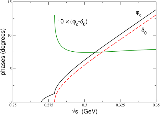
  Figure 8: The phases $\varphi_{c}$ and $\delta_{0}$, as well as their difference. The cusp in the phase $\varphi_{c}$ at the charged threshold $s=4M_{\pi}^{2}$ is clearly visible. The isospin-symmetric parts $\bar{d}_{i}$ have been determined from the matching condition, Eqs. (42) and (43), with the scattering lengths and effective radii taken from Ref. [2]. The isospin breaking corrections $d_{i}^{\prime}$ were evaluated in ChPT at $O(p^{2})$, see Eq. (5.2). The ratio $f_{0}/f_{c}$ was set to one.

• The standard way to define the phase of the form factor on the real axis in the interval $s\geq 4M_{\pi^{0}}^{2}$ is

  $$\varphi_{c}=\arctan\frac{\mbox{Im}\,F_{c}(s+i0)}{\mbox{Re}\,F_{c}(s+i0)}\,.$$ (49)

  The quantity $\varphi_{c}$ does not vanish at the charged threshold $s=4M_{\pi}^{2}$ and has a cusp there. This is illustrated in Fig. 8, where the phase $\varphi_{c}$ is plotted. For comparison, the isospin-symmetric phase $\delta_{0}$ and the difference $\varphi_{c}-\delta_{0}$ are displayed as well. The phases $\theta_{c}$ and $\varphi_{c}$ are identical on the real axis above the charged threshold,

  $$\varphi_{c}(s)=\theta_{c}(s)\,,\quad\quad s\geq 4M_{\pi}^{2}\,.$$ (50)

  On the other hand, they differ e.g. in the interval $s\in[4M_{\pi^{0}}^{2},4M_{\pi}^{2}]$, because $\theta_{c}(s)$ becomes complex there.

5.2 Form factor of pion: chiral expansion

We calculate the scalar form factor of the pion in the $SU(2)$ version of ChPT. The Lagrangian is given by [20]

$${\cal L}={\cal L}_{2}+{\cal L}_{4}\,,$$ (51)

where

$${\cal L}_{2}=\frac{F^{2}}{4}\langle\partial_{\mu}U\partial^{\mu}U^{\dagger}+2Bs(U+U^{\dagger})\rangle+C\langle QUQU^{\dagger}\rangle\,.$$ (52)

In the above expression we use standard notations. In particular, $F$ denotes the pion decay constant in the chiral limit, $U$ is the pion field matrix, the quantity $B$ is related to the quark condensate, $s={\cal M}+s^{\prime}$ is the scalar source, ${\cal M}$ and $Q$ stand for the quark mass and charge matrices in the $SU(2)$ case, respectively, and the coupling $C$ is proportional to $\Delta_{\pi}$ at lowest order in the chiral expansion. In accordance to the discussion in section 3, we do not include virtual photons.

We do not display the order $p^{4}$ Lagrangian ${\cal L}_{4}$ explicitly. It is given, e.g., in Refs. [20]. Note that, since we do not include virtual photons, the ultraviolet divergences of the “electromagnetic” LECs $k_{i}$ from Refs. [20] change in an obvious manner.

In the calculations, the scalar current $j(x)=(2B)^{-1}(\bar{u}(x)u(x)+\bar{d}(x)d(x))$ was used. The scalar form factors of the pion at one loop can be calculated in a standard manner and are given by the following expressions,

$$F_{c}(s) = 1+\frac{1}{2F^{2}}\,\biggl{\{}(s+4\,\Delta_{\pi})\bar{J}(s)+(s-M_{\pi^{0}}^{2})\bar{J}_{0}(s)\biggr{\}}$$

$$+ \frac{1}{32\pi^{2}F^{2}}\,\biggl{\{}-(s+4\,\Delta_{\pi})(L+1)-(s-M_{\pi^{0}}^{2})(L_{0}+1)+M_{\pi^{0}}^{2}L_{0}\biggr{\}}$$

$$+ \frac{4M_{\pi^{0}}^{2}}{F^{2}}\,l_{3}^{r}+\frac{s}{F^{2}}\,l_{4}^{r}+e^{2}{\cal K}_{c}^{r}+O(p^{4})\,,$$

$$F_{0}(s) = 1+\frac{1}{2F^{2}}\,\biggl{\{}2(s-M_{\pi^{0}}^{2})\bar{J}(s)+M_{\pi^{0}}^{2}\bar{J}_{0}(s)\biggr{\}}$$ (53)

$$+ \frac{1}{32\pi^{2}F^{2}}\,\biggl{\{}-2(s-M_{\pi^{0}}^{2})(L+1)-M_{\pi^{0}}^{2}(L_{0}+1)+2M_{\pi}^{2}L-M_{\pi^{0}}^{2}L_{0}\biggr{\}}$$

$$+ \frac{4M_{\pi^{0}}^{2}}{F^{2}}\,l_{3}^{r}+\frac{s}{F^{2}}\,l_{4}^{r}+e^{2}{\cal K}_{0}^{r}+O(p^{4})\,.$$

Here

$$L=\ln\frac{M_{\pi}^{2}}{\mu^{2}}\,,\quad\quad L_{0}=\ln\frac{M_{\pi^{0}}^{2}}{\mu^{2}}\,,$$ (54)

and the loop function $\bar{J}(s)$ is displayed in Eq. (2) [$\bar{J}_{0}$ is obtained from it by the replacement $\sigma\to\sigma_{0}$]. Further,

$${\cal K}_{c}^{r} = -\frac{20}{9}\,(k_{1}^{r}+k_{2}^{r})+\frac{4}{9}\,(5k_{5}^{r}+23k_{6}^{r}+k_{7}^{r})+8k_{8}^{r}\,,$$

$${\cal K}_{0}^{r} = -\frac{20}{9}\,(k_{1}^{r}+k_{2}^{r})-2(-2k_{3}^{r}+k_{4}^{r})+\frac{4}{9}\,(5k_{5}^{r}+5k_{6}^{r}+k_{7}^{r})\,.$$ (55)

In these expressions $l_{i}^{r}$ and $k_{i}^{r}$ denote scale-dependent renormalized LECs, the $k_{i}^{r}$ adapted to the framework considered here (no photon loops). The quantity $\mu$ is the scale of dimensional regularization in ChPT.

The scalar form factor of the pion in the presence of isospin breaking have been evaluated in Ref. [29]. Our expressions agree with those of Ref. [29] up to contributions of virtual photons and terms of order $e^{4}$, $e^{2}(m_{d}-m_{u})$ and $(m_{d}-m_{u})^{2}$.

The phase of the charged form factor at one loop, extracted from Eq. (53), is given by

$$\theta_{c}(s)=\frac{1}{32\pi F^{2}}\left\{(4\Delta_{\pi}+s)\sigma+(s-M_{\pi^{0}}^{2})\sigma_{0}\right\}\,.$$ (56)

It is seen that $\theta_{c}$ indeed does not vanish at the threshold $s=4M_{\pi}^{2}$.

Next we determine the non-relativistic couplings $d_{i},f_{k}$, performing the matching to ChPT at $O(p^{2})$. We start from $d_{i}$, which can be directly read off from the tree–level S-wave $\pi\pi$ scattering amplitudes:

$$d_{c}(s) = \frac{s+4\Delta_{\pi}}{128\pi F^{2}}+O(p^{4})\,,\,$$

$$d_{x}(s) = -\frac{s-M_{\pi^{0}}^{2}}{64\pi F^{2}}+O(p^{4})\,,\,$$

$$d_{0}(s) = \frac{M_{\pi^{0}}^{2}}{64\pi F^{2}}+O(p^{4})\,.$$ (57)

The quantities $f_{k}$ at $O(p^{2})$ can be determined by performing the matching to the one–loop expressions for the form factors, given in Eq. (53). For the ratio $f_{0}/f_{c}$ one gets

$$\frac{f_{0}}{f_{c}} = H_{0}+H_{1}(s-4M_{\pi}^{2})+O((s-4M_{\pi}^{2})^{2})\,,\quad\quad$$

$$H_{0} = 1+\frac{3\Delta_{\pi}L}{16\pi^{2}F^{2}}+e^{2}({\cal K}_{0}^{r}-{\cal K}_{c}^{r})+O(\Delta_{\pi}^{2},p^{4})\,,$$

$$H_{1} = \frac{\Delta_{\pi}}{12\pi^{2}F^{2}M_{\pi}^{2}}+O(\Delta_{\pi}^{2},p^{2})\,.$$ (58)

We note that in the case of isospin violation the ratio $f_{0}/f_{c}$ is not determined only by the LECs that enter the $\pi\pi$ amplitude. For example, even in the chiral limit the ratio $f_{0}/f_{c}$ contains the LEC $k_{8}$, which is absent from the $\pi\pi$ amplitudes in this limit. Consequently, in the case of broken isospin, the phase of the form factors is not determined by the $\pi\pi$ scattering amplitudes alone.

It is easy to check that the expression for the phase Eq. (56) can be directly obtained from Eq. (48) by using the result of the tree–level matching, given in Eq. (5.2). At this order, one may take $f_{0}/f_{c}=1+O(p^{2})$.

In order to check the convergence of the chiral expansion, we have evaluated the phase of the charged form factor at two loops. We do not display the final result here. As expected, the next-to-leading correction lies within approximately $30\%$ of the leading-order result, see section 7 for a more quantitative result.

6 $K_{e4}$ decays: isospin breaking

We now come back to the analysis of $K_{e4}$ decays. We simply need to repeat the above analysis, this time for the matrix element Eq. (3) of the axial current.

Working out the contributions from diagrams Figs. 1 and 2, one finds that the phase $\psi_{0}$ of the form factor $f_{0}$ [see Eq. (16)] becomes in the elastic region $4M_{\pi}^{2}<s<16M_{\pi^{0}}^{2}$

$$\psi_{0}=\frac{1}{32\pi F^{2}}\left\{(4\Delta_{\pi}+s)\sigma+(s-M_{\pi^{0}}^{2})\left(1+\frac{3}{2R}\right)\sigma_{0}\right\}+O(p^{4})\,,$$ (59)

with

$$R=\frac{m_{s}-\hat{m}}{m_{d}-m_{u}}\,,$$ (60)

and $F$ the pion decay constant in the $SU(2)$ chiral limit. The phase of the form factor $f_{1}$ does not contain at this order any isospin breaking effects [these are generated by $\pi^{0}\pi^{0}$ intermediate states, which cannot couple to P-waves], as a result of which one has

$$\psi_{1}=\delta_{1}$$ (61)

at this order in the low–energy expansion. The one–loop expressions for the form factors $F,G$ given in Refs. [16] contain the effects considered here, up to terms of order $e^{2}(m_{d}-m_{u})$.

Figure 9: The isospin breaking correction that must be subtracted from the phase shift $\delta$ measured in $K_{e4}$ decays. The width of the band reflects the uncertainty in the ratio $R=37\pm 5$.

We comment on this result. First, in comparison to the pion form factor discussed above, there is an additional term present, proportional to $m_{d}-m_{u}$. This is in agreement with the statement made before: the phase is not fixed by the $\pi\pi$ amplitude alone, which does not contain any $m_{d}-m_{u}$ terms at one–loop order. Second, the difference to the isospin symmetric phase now grows with $s$ even at one–loop order,

$$\psi_{0}-\delta_{0} = \frac{3s}{64\pi F^{2}}\frac{1}{R}+O(1)\,,\quad s/M_{\pi}^{2}\gg 1\,.$$ (62)

According to the discussion in section 3, one has to subtract the difference $\psi_{0}-\delta_{0}$ from the measured phase shift before a comparison with the chiral prediction can be performed. In figure 9 we display this difference in the relevant decay region, for $R=37\pm 5$. The width of the band reflects the uncertainty in $R$. It is seen that the isospin correction is quite substantial – well above the systematic and statistical uncertainties quoted for the measured phase shift [7].

In addition, similarly to the case of the scalar form factor, the phase–removed form factor for the $K_{e4}$ decays is not holomorphic at the charged threshold and, consequently, in the expansion of this form factor even and odd powers of the variable $q$ are present, in contrast to the isospin symmetric case, see Eq. (10). If the value of the form factor at $q=0$ is factored out, the coefficient of the term linear in $q$ is the same as in the case of the scalar form factor at leading order in ChPT. On the other hand, this is a two–loop effect and therefore suppressed in magnitude. To obtain a reliable estimate of its size is beyond the scope of this work.

7 $\pi\pi$ scattering lengths from $K_{e4}$ decays

The first large-statistics experiment to measure the phase $\psi_{0}-\psi_{1}$ in $K_{e4}$ decays has been performed by the Geneva-Saclay collaboration about thirty years ago. In this experiment about 30’000 $K_{e4}$ decays have been collected and analysed [4]. More recently the E865 experiment at Brookhaven [4] and the NA48/2 experiment at CERN [5] have each collected more than ten times the statistics and have made possible a precise extraction of the scattering length $a_{0}^{0}$. So precise in fact, that a proper treatment of the isospin breaking corrections as discussed in this paper becomes essential.

In this section we discuss how the isospin breaking corrections influence the extraction of the scattering length, and will do this for all three data sets. We perform two kinds of analyses: we will either leave both S-wave scattering lengths free and fit them to the data, or use a low–energy theorem which relates both of them to the scalar radius of the pion and end up with a one–parameter fit [30].

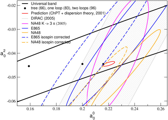
Figure 10: S-wave scattering lengths plane. Contours shown correspond to one sigma. The ellipses do not take into account any theoretical uncertainty.

For the two–parameter fits we have used the parametrization of the $\pi\pi$ phase shifts corresponding to solutions of the Roy equations as functions of the two S-wave scattering lengths which was provided in [31]. To evaluate numerically the isospin breaking correction (59) we have used $R=37\pm 5$ and $F=86.2\pm 0.5$ MeV [32] – moreover we use the fact that $\psi_{1}=\delta_{1}$ at one–loop order. The results of these fits are shown in Fig. 10 as one–sigma contours (68% probability, i.e. $\chi^{2}=\chi^{2}_{\mathrm{min}}+2.31$) for the two most recent data sets, with and without taking into account isospin-breaking corrections. The ellipses corresponding to the Geneva-Saclay data are too large in comparison and for this reason we have not shown them in the same figure. The figure shows that while the ellipse corresponding to the uncorrected NA48 data does not overlap with the theoretical prediction, after applying the isospin breaking correction, the two overlap completely. For the ellipses corresponding to the E865 data the situation is reversed: before applying isospin breaking corrections there is a perfect overlap, whereas after applying them the experimental one–sigma contour and the theory prediction barely touch. The figure also clearly shows that the two sets of very high statistics data are not in very good mutual agreement: the two one–sigma ellipses (with or without isospin breaking corrections) do not have any significant overlap. It has been recently pointed out by Brigitte Bloch-Devaux that the origin of this tension lies in the data point in the last bin of the E865 data set [7], for which the evaluation of the barycenter may need to be revised [33]: we have verified that indeed it is enough to remove this point from the fit to obtain an almost perfect overlap between the two ellipses.

We take into account the constraint of the pion scalar radius as follows: we use the numerical estimate $\langle r^{2}\rangle_{s}=0.61\pm 0.04$ fm² [2], which implies the relation

$$a_{0}^{2} = f(\Delta a_{0}^{0})\pm 0.0008\,,\,\qquad\Delta a_{0}^{0}\equiv a_{0}^{0}-0.22\,,\,$$

$$f(x) = -0.0444+0.236\,x-0.61\,x^{2}-9.9\,x^{3}\,,\,$$ (63)

where the error accounts for the various sources of uncertainty in the input used in the Roy equation solutions. In our fits we minimize the following $\chi^{2}$:

$$\chi^{2}_{\mathrm{tot}}=\left(\frac{a_{0}^{2}-f(\Delta a_{0}^{0})}{0.0008}\right)^{2}+\chi^{2}_{K_{e4}}\;\;.$$ (64)

Since the $K_{e4}$ data are very little sensitive to $a_{0}^{2}$, the minimum of the $\chi^{2}$ lies then always on the $f(\Delta a_{0}^{0})$ line, but in this way we also take into account the uncertainty in the scalar radius relation. The results of the fits are:
without applying isospin breaking corrections

$$a_{0}^{0}=\left\{\begin{array}[]{lllll}0.243\pm 0.037&&\chi^{2}=2.2&\mbox{Geneva-Saclay}&\mbox{[ $\,$5 data pts.]}\\ 0.218\pm 0.013&&\chi^{2}=5.8&\mbox{E865}&\mbox{[ $\,$6 data pts.]}\\ 0.245\pm 0.007&&\chi^{2}=9.6&\mbox{NA48}&\mbox{[10 data pts.]}\,,\\ \end{array}\right.$$ (65)

and after applying isospin breaking corrections

$$a_{0}^{0}=\left\{\begin{array}[]{llll}0.222\pm 0.040&&\chi^{2}=2.1&\mbox{Geneva-Saclay}\\ 0.195\pm 0.013&&\chi^{2}=6.6&\mbox{E865}\\ 0.223\pm 0.007&&\chi^{2}=11.5&\mbox{NA48}\,.\\ \end{array}\right.$$ (66)

Averaging the latter three independent determinations yields $a_{0}^{0}=0.217\pm 0.008$ where the error has been inflated by an $S=1.3$ factor according to the PDG prescription (the $\chi^{2}$ of the average of the three fits is equal to 6.3). Repeating the same procedure after having removed the last data point in the E865 set yields $a_{0}^{0}=0.221\pm 0.007$ with $\chi^{2}\simeq 0.7$, so confirming the observation of Brigitte Bloch-Devaux [7]. We also briefly comment on the vertex corrections at order $\alpha_{QED}$ mentioned in section 3. They lower the value of $a_{0}^{0}$ by $\simeq 0.013$. For reasons already mentioned, we do not take these corrections into account in the present work.

The extraction of the scattering length $a_{0}^{0}$ from the phase shift $\psi_{0}-\psi_{1}$ measured in $K_{e4}$ data requires theory input in two steps: the first is the subject of this article, the evaluation of the isospin breaking corrections which lead from $\psi_{0}-\psi_{1}$ to $\delta_{0}-\delta_{1}$, and the second is the step from the phase $\delta_{0}-\delta_{1}$ to the scattering length. Both steps can be made quite accurately, but both are subject to a theory uncertainty which, though small, has to be properly accounted for at the level of precision currently reached by experiments. As far as step one is concerned, the evaluation of the isospin breaking correction given in Eq. (59) relies on an estimate of $F$ and $R$ as discussed above. A one–sigma change in $F$ has no visible effect in the fitted value of $a_{0}^{0}$, whereas a change of $R$ by five units shifts $a_{0}^{0}$ by $0.001$. Our one–loop estimate of these effects is subject to higher–order corrections. We have evaluated these in the case of the scalar form factor of the pion discussed in previous sections. If we use the latter as our estimate of higher–order isospin breaking effects and repeat the fits, we get a value of $a_{0}^{0}$ shifted by $0.004$. An alternative quick way to estimate two–loop effects is to substitute $F$ with the physical $F_{\pi}$ – doing this the fitted value of the scattering length changes by 0.003. We conclude that $0.004$ is a reasonable estimate of the uncertainty due to higher–order isospin breaking corrections. As for step two, the main source of uncertainty in the calculation of how the Roy equation solution depend on $a_{0}^{0}$ is represented by the value of the $\delta_{0}$ phase at 0.8 GeV [31], which had been estimated to be $(82.3\pm 3.4)^{\circ}$. Changing the latter by one sigma and repeating the fits leads to a shift of $a_{0}^{0}$ by 0.004. If we sum in squares these four different sources of uncertainty (namely: value of $F$, value of $R$, higher–order isospin breaking corrections and value of $\delta_{0}(0.8\mbox{GeV})$ we end up with

$$a_{0}^{0}=0.217\pm 0.008_{\mathrm{exp}}\pm 0.006_{\mathrm{th}}\;\;,$$ (67)

which represents the current best experimental determination of the isospin zero S-wave scattering length coming from $K_{e4}$ decays. NA48 is currently analysing more statistics [7], and we expect that when the updated analysis will become available, the experimental error will reach or even become smaller than the theoretical one. Other competitive determinations coming from the cusp in $K\to 3\pi$ decays [10] and from pionium lifetime [9] are also expected to be improved in the near future.

8 Comparison with other work

The isospin-breaking corrections to the $K_{e4}$ decays have been evaluated in the past by using various theoretical settings. We briefly review some recent articles where the problem has been addressed.

In Ref. [16], a full set of isospin-breaking corrections to the $K_{e4}$ decays of charged kaons has been calculated at one loop in ChPT. Our result for the elastic phase shift given in Eq. (59) agrees with the result of Refs. [16] in the absence of virtual photon contributions. As already mentioned in section 3, these calculations might provide a basis for an algorithm which removes isospin-breaking corrections from the raw experimental data.

In Refs. [13, 14], isospin-breaking corrections to $K_{e4}$ decays have been treated in an approach which may be considered a merger between $K$-matrix theory and a conventional quantum-mechanical framework used to study Coulomb interactions in the final state. Although some of the expressions in Refs. [13, 14] closely resemble the pertinent formulae of the present work, the framework used is incomplete and, as far as we can see, incorrect. To mention two examples, we note that a relation between the amplitude considered there and the $K_{e4}$ decay matrix element is not provided, and the effect caused by the quark mass difference $m_{d}-m_{u}$ is not discussed at all. Moreover, according to the explicit formulae given in Refs. [14], the effect of isospin breaking – in the absence of Coulomb interactions – can be expressed through the S-wave $\pi\pi$ scattering phases (in the isospin limit) and the pion mass difference. As we show in the present article, this is not correct. The authors of Refs. [13, 14] also provide a set of electromagnetic corrections which include both, vertex corrections and rescattering of the virtual pions through the exchange of Coulomb photons (the latter is a two–loop effect in our terminology). As already mentioned, it is not clear which part of these corrections was already taken into account in present analyses. We conclude that one should not use the results of Refs. [13, 14] in data analyses of $K_{e4}$ decays.

9 Summary and conclusions

Data on $K_{e4}$ decays allow one to measure the difference of the S- and P-wave phases $\psi_{0}-\psi_{1}$ of a particular form factor in the matrix element of the strangeness-changing axial current. If isospin symmetry were exact, $\psi_{0}-\psi_{1}$ would coincide with the difference of the S- and P-wave $\pi\pi$ scattering phase shifts $\delta_{0}-\delta_{1}$ (Watson’s theorem). We have shown that the situation changes if isospin symmetry is broken. In particular,

• The phases $\psi_{0}$ and $\delta_{0}$ are not equal. Moreover, $\psi_{0}$ is not determined by the $\pi\pi$ scattering amplitudes alone (e.g., the former contains the LECs which are absent in the latter).

• The phase $\psi_{0}$ does not vanish at the threshold $s=4M_{\pi}^{2}$.

• At threshold, the expansion in Eq. (10), which is valid in the isospin symmetry limit, becomes $e^{-i\psi_{0}}f_{0}(s,s_{\ell})=\bar{c}_{0}+\bar{c}_{1}q+\bar{c}_{2}q^{2}+O(q^{3})\,,\,$ where the coefficients $\bar{c}_{i}$ depend on the variable $s_{\ell}$, and similarly for the P-wave form factor $f_{1}$ (although at higher order in the chiral expansion).

Finally, in order to determine the isospin symmetric phases from data, one uses Eq. (17) and calculates the difference $\psi_{k}-\delta_{k}$, which must then be subtracted from the measured phases $\psi_{k}$. We have performed this calculation at one loop in ChPT for $K_{e4}$ decays and have shown that the correction is substantial, well above the statistical and systematic errors in present NA48/2 data. Once this is taken into account, the determination of the isospin zero S-wave scattering length from $K_{e4}$ data yields

$$a_{0}^{0}=0.217\pm 0.008_{\mathrm{exp}}\pm 0.006_{\mathrm{th}}\;\;,$$

in excellent agreement with the chiral prediction.

Acknowledgments

We are grateful to the late F.J. Ynduráin for useful comments at an early stage of this work. We thank all participants of the $K_{e4}$ workshop in Bern (March 2007) for interesting discussions, which have inspired the present investigations. We thank B. Ananthanarayan, B. Bloch–Devaux, I. Caprini, S. Gevorkyan, Ch. Hanhart, Ulf-G. Meißner, B. Kubis, H. Leutwyler, J. Peláez, and Z. Was for most enjoyable discussions, and A.V. Tarasov for communications concerning topics considered here. We are grateful to B. Bloch-Devaux for useful comments concerning the manuscript, and for performing extensive fits which cross-checked our results for the scattering lengths. The Center for Research and Education in Fundamental Physics is supported by the “Innovations- und Kooperationsprojekt C-13” of the “Schweizerische Universitätskonferenz SUK/CRUS”. Partial financial support under the EU Integrated Infrastructure Initiative Hadron Physics Project (contract number RII3–CT–2004–506078) and DFG (SFB/TR 16, “Subnuclear Structure of Matter”) is gratefully acknowledged. This work was supported by the Swiss National Science Foundation, and by EU MRTN–CT–2006–035482 (FLAVIAnet).

Appendix A Notation

In the main text, we use the following notation for cut complex planes:

$$\mathbb{C}_{LR}(a) = \left\{z|z\in\mathbb{C},z\not\in(-\infty,0],z\not\in[a,\infty)\right\}\,,\,$$

$$\mathbb{C}_{R}(a) = \left\{z|z\in\mathbb{C},z\not\in[a,\infty)\right\}\,.$$ (A.1)

• The region $\mathbb{C}_{LR}(a)$ denotes the complex plane, cut along the negative real axis, as well as along the positive real axis for $z\geq a$.

• The region $\mathbb{C}_{R}(a)$ denotes the complex plane, cut along the positive real axis for $z\geq a$.

Appendix B Threshold behaviour of phases and form factors

We prove some of the statements made in section 4 and start with the isospin symmetric case considered in subsection 4.1. The issue was discussed in the literature long ago [24] – we keep the presentation therefore short.

B.1 Isospin symmetric case

The partial waves are denoted by $t_{k}$. We assume that these i) are holomorphic in the cut plane $C_{I}$ shown in Fig. B.1, ii) are real on the real axis $0<s<4M_{\pi}^{2}$, and iii) converge to continuous boundary values $t_{k}(s)$ as $z\to s$. The form factors are boundary values of functions $F_{k}(z)$ which are assumed to be i) holomorphic in the complex $z$-plane, cut at $z=s$ for $s\geq 4M_{\pi}^{2}\,,\,$ ii) real on the real axis for $s<4M_{\pi}^{2}\,,\,$ iii) nonzero for finite $|z|$. Furthermore, we assume that $F_{k}(z)$ converge to continuous boundary values $F_{k}(s)$ as $z\to s$.

cut plane $C_{I}$                                                             
                                                                          cut plane $C_{II}$

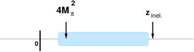
region $C_{III}$

Figure B.1: Regions of analyticity in the complex $z$–plane, isospin symmetric case. We assume that $t_{k}$ are holomorphic in the cut plane $C_{I}$. The two-particle irreducible amplitude $t$ is then meromorphic in the cut plane $C_{II}$, and the phase–removed form factor $\hat{F}_{c}$ is holomorphic in the shaded region $C_{III}$. The symbol $z_{inel}$ denotes the inelastic threshold $z=16M_{\pi}^{2}$.

We introduce the two–particle irreducible amplitude

$$t(z)=\frac{t_{0}(z)}{1+i\sigma(z)t_{0}(z)}\,.$$ (B.2)

It is meromorphic in $C_{I}$. The poles are due to possible zeros in the denominator. In the elastic region, the discontinuity of $t$ vanishes. ¿From the Edge-of-the-Wedge theorem (EWT) it then follows that $t$ is meromorphic in the cut plane $C_{II}$ displayed in Fig. B.1. Solving for $t_{0}$ gives

$$t_{0}(z) = F(z)+i\sigma G(z)\,\,$$

$$F = \frac{t}{1+\sigma^{2}t^{2}}\,,\,G=tF\,.$$ (B.3)

The quantities $F,G$ are meromorphic in $C_{II}$. From this representation, it follows that the analytic continuation of $t_{0}$ to the second Riemann sheet is [24]

$$t_{0}^{(2)}=\frac{t_{0}}{1+2i\sigma t_{0}}\,,\,$$ (B.4)

which shows that the zeros of the $S$-matrix on the first Riemann sheet correspond to poles of the partial waves on the second Riemann sheet, at the same value of $z$.

Now consider the form factor $F_{c}$, and define the ratio

$$R(z)=\frac{F_{c}(z)}{t_{0}(z)}\,,\,$$ (B.5)

which is meromorphic in $C_{I}$. Unitarity and EWT show that the elastic cut is absent. Therefore, one has the decomposition

$$F_{c}(z)=A(z)+i\sigma B(z)\,,\,$$ (B.6)

with $A,B$ meromorphic in $C_{II}$. Furthermore, the form factor generates a pole on the second Riemann sheet as well, at the same place where $t_{0}$ does. Finally, the phase defined in Eq. (33) coincides with the isospin zero S–wave $\pi\pi$ phase shift in the elastic interval, because $R$ is real there. The phase–removed form factor in Eq. (34) is holomorphic in the shaded region $C_{III}$ displayed in Fig. (B.1).

B.2 Isospin broken case

The threshold structure of the form factor displayed in Eq. (36) can be obtained in a manner quite analogously to the previous subsection. One first works out the threshold behaviour of the scattering amplitudes. We assume that the $h_{k}$ i) are holomorphic in the region $D_{I}$ displayed in Fig. B.2, ii) are real on the real axis in the interval $0<s<4M_{\pi^{0}}^{2}$, and ii) converge to continuous boundary values $h_{k}(s)$ as $z\to s$. The form factors $F_{k}$ are assumed to satisfy the same conditions as above, with $M_{\pi}^{2}\to M_{\pi^{0}}^{2}$.

cut plane $D_{I}$                                                             
                                                                          cut plane $D_{II}$

region $D_{III}$

Figure B.2: Regions of analyticity in the complex $z$-plane, isopin broken case. We assume that $t_{k}$ are holomorphic in the cut plane $D_{I}$. The two-particle irreducible amplitude $\hat{T}$ is meromorphic in the cut plane $D_{II}$, and the phase–removed form factor $\hat{F}_{c}$ is holomorphic in the shaded region $D_{III}$, with the cut indicated. The symbol $z_{inel}$ denotes the inelastic threshold $z=16M_{\pi^{0}}^{2}$.

We introduce the matrix

$$\bar{\rho}(z)=\left(\!\!\begin{array}[]{cc}2\sigma(z)&0\\ 0&\sigma_{0}(z)\end{array}\!\!\right)\,,\,$$ (B.9)

compare the comments after Eq. (29). Consider the two–particle irreducible amplitudes

$$\hat{T}=\left(1+iT\bar{\rho}\right)^{-1}T\,,\,$$ (B.10)

where the matrix $T$ is defined in Eq. (25). Unitarity and EWT show that the cut $4M_{\pi^{0}}^{2}<s<16M_{\pi^{0}}^{2}$ is absent for $\hat{T}$, from where we conclude that the matrix $T$ has the threshold structure

$$T=A^{\prime}+i\sigma B^{\prime}+i\sigma_{0}C^{\prime}+\sigma\sigma_{0}D^{\prime}$$ (B.11)

with matrices $A^{\prime},B^{\prime},C^{\prime},D^{\prime}$ whose entries are meromorphic in $D_{II}$. Next, one forms

$$\left(\!\!\begin{array}[]{c}R_{c}\\ R_{0}\end{array}\!\!\right)=T^{-1}F\,,\,$$ (B.14)

where $F$ is the matrix in Eq. (25), and uses again unitarity and EWT to show that $R_{c,0}$ are meromorphic in $D_{II}$. Solving for $F$ gives

$$F_{k}=A_{k}+i\sigma B_{k}+i\sigma_{0}C_{k}+\sigma\sigma_{0}D_{k}\,;\,k=c,0\,,\,$$ (B.15)

with $A_{k},\cdots,D_{k}$ meromorphic in $D_{II}$. Evaluating the phases $\theta_{k}$ according to Eq. (37) shows that these depend on the ratio $R_{0}/R_{c}$. On the other hand, this ratio depends on $F_{c}/F_{0}$, which is unity in the isospin limit, and different otherwise. In subsection 5.2 we show that, in case of ChPT, $F_{c}/F_{0}$ contains LECs that do not occur in the $\pi\pi$ scattering amplitude. Hence the phases $\theta_{k}$ are not determined by the $\pi\pi$ amplitude alone in the case of broken isospin. From (37), it is seen that the phase $\theta_{c}$ does not vanish at the threshold $s=4M_{\pi}^{2}$, because $\sigma_{0}(4M_{\pi}^{2})\neq 0$. Finally, from Eq. (B.15), one finds for the phase–removed form factor the result

$$\hat{F}_{c}=(A_{c}+\sigma\sigma_{0}D_{c})\left[1+\left(\frac{\sigma B_{c}+\sigma_{0}C_{c}}{A_{c}+\sigma\sigma_{0}D_{c}}\right)^{2}\right]^{\frac{1}{2}}\,.$$ (B.16)

It is holomorphic in the cut region $D_{III}$ displayed in Fig. B.2. The cut is due to the factor $\sigma\sigma_{0}$.

Appendix C Non-relativistic effective Lagrangian framework

The non-relativistic Lagrangian ${\cal L}={\cal L}_{\pi\pi}+{\cal L}_{\cal O}$, which is used for calculation of the scalar form factor, consists of a part describing quartic pion-pion interactions, and a part corresponding to the interaction of the pion pair with the external current ${\cal O}(x)$. The framework is described in detail in our recent works [25, 26, 27] and will not be repeated here. For example, the Lagrangian ${\cal L}_{\pi\pi}$ is given in Eq. (4) of Ref. [25]. The polynomials $d_{i}(z)$, introduced in section 5.1, are given by

$$32\pi d_{c} = C_{+-}+(z-4M_{\pi}^{2})D_{+-}\,,$$

$$32\pi d_{x} = C_{x}+(z-4M_{\pi}^{2})D_{x}\,,$$

$$32\pi d_{0} = C_{00}+(z-4M_{\pi^{0}}^{2})D_{00}\,.$$ (C.17)

Here we use the same notations for the 4-pion couplings $C,D$ as in Refs. [25, 26, 27]. The matching of these couplings to the effective-range expansion parameters in the $\pi\pi$ scattering amplitudes is described in these references as well.

The part of the Lagrangian which is responsible for the interaction with the external source takes the form

$${\cal L}_{\cal O} = {\cal O}\,\biggl{(}-f_{1}\Phi_{+}^{\dagger}\Phi_{-}^{\dagger}+f_{2}(W_{\pm}\Phi_{+}^{\dagger}W_{\pm}\Phi_{-}^{\dagger}+\nabla\Phi_{+}^{\dagger}\nabla\Phi_{-}^{\dagger}-M_{\pi}^{2}\Phi_{+}^{\dagger}\Phi_{-}^{\dagger})$$ (C.18)

$$+ \frac{f_{3}}{2}\,\Phi_{0}^{\dagger}\Phi_{0}^{\dagger}-\frac{f_{4}}{2}\,(W_{0}\Phi_{0}^{\dagger}W_{0}\Phi_{0}^{\dagger}+\nabla\Phi_{0}^{\dagger}\nabla\Phi_{0}^{\dagger}-M_{\pi^{0}}^{2}\Phi_{0}^{\dagger}\Phi_{0}^{\dagger})\biggr{)}+\mbox{h.c.}\,.$$

where $\Phi_{\pm},\Phi_{0}$ denote the non-relativistic charged and neutral pion fields, $W_{\pm}=\sqrt{M_{\pi}^{2}-\triangle}$ and $W_{0}=\sqrt{M_{\pi^{0}}^{2}-\triangle}$ are the pertinent differential operators, and $f_{1},\cdots f_{4}$ stand for the various non-relativistic couplings. The polynomials $f_{c},f_{0}$ which are used in the main text are defined as

$$f_{c}=f_{1}-\frac{1}{2}\,(z-4M_{\pi}^{2})f_{2}\,,\quad\quad f_{0}=f_{3}-\frac{1}{2}\,(z-4M_{\pi^{0}}^{2})f_{4}\,.$$ (C.19)

In order to calculate the scalar form factors within the non-relativistic framework, one evaluates the transition amplitude between the non-relativistic two–pion states and the vacuum in the presence of the external source ${\cal O}(x)$. The form factors are defined by

$$\langle\pi^{+}(p_{1})\pi^{-}(p_{2});\mbox{out}|0;\mbox{in}\rangle_{\cal O}^{NR} = i\int d^{4}x{\rm e}^{i(p_{1}+p_{2})x}{\cal O}(x)\,F_{c}(s)+O({\cal O}^{2})\,,$$

$$\langle\pi^{0}(p_{1})\pi^{0}(p_{2});\mbox{out}|0;\mbox{in}\rangle_{\cal O}^{NR} = i\int d^{4}x{\rm e}^{i(p_{1}+p_{2})x}{\cal O}(x)\,F_{0}(s)+O({\cal O}^{2})\,,$$

where $s=(p_{1}+p_{2})^{2}$.

The behaviour of both the relativistic and non-relativistic form factors at small momenta is the same and is displayed in Eq. (36). The polynomials $f_{k}$ can be determined by performing a matching of the regular part $A_{k}$ of the form factors, evaluated in both theories.

References

- [1] S. Weinberg, Physica A 96 (1979) 327.
- [2] G. Colangelo, J. Gasser and H. Leutwyler, Nucl. Phys. B 603 (2001) 125 [arXiv:hep-ph/0103088].
- [3] G. Colangelo, “Theoretical progress on pi pi scattering lengths and phases,” Talk given at Kaon International Conference (KAON’07), Frascati, Italy, 21-25 May 2007, PoS KAON (2008) 038 [arXiv:0710.3050 [hep-ph]].
- [4] L. Rosselet et al., Phys. Rev. D 15 (1977) 574; S. Pislak et al. [BNL-E865 Collaboration], Phys. Rev. Lett. 87 (2001) 221801 [arXiv:hep-ex/0106071]; S. Pislak et al. [BNL-E865 Collaboration], Phys. Rev. D 67 (2003) 072004 [arXiv:hep-ex/0301040].
- [5] J. R. Batley et al. [NA48/2 Collaboration], Eur. Phys. J. C 54 (2008) 411.
- [6] B. Bloch-Devaux, Recent results from NA48/2 on K(e4) decays and interpretation in term of scattering lengths, PoS KAON (2008) 035.
- [7] B. Bloch-Devaux, Results from NA48/2 decays: Form Factors and scattering lengths, talk given at: FlaviaNet Kaon Workshop, Anacapri, Italy, June 12-14, 2008.
-
[8]
For talks provided by members of the NA48/2 collaboration, see
http://na48.web.cern.ch/NA48/Welcome/images/talks.html - [9] B. Adeva et al. [DIRAC Collaboration], J. Phys. G 30 (2004) 1929 [arXiv:hep-ex/0409053]; B. Adeva et al. [DIRAC Collaboration], Phys. Lett. B 619 (2005) 50 [arXiv:hep-ex/0504044].
- [10] J. R. Batley et al. [NA48/2 Collaboration], Phys. Lett. B 633 (2006) 173 [arXiv:hep-ex/0511056]; E. Abouzaid et al. [The KTeV Collaboration], arXiv:0806.3535 [hep-ex].
- [11] E. Barberio, B. van Eijk and Z. Was, Comput. Phys. Commun. 66 (1991) 115; E. Barberio and Z. Was, Comput. Phys. Commun. 79 (1994) 291; G. Nanava and Z. Was, Eur. Phys. J. C 51 (2007) 569 [arXiv:hep-ph/0607019].
- [12] J. Gasser and A. Rusetsky, Isospin violations in decays, Internal note to the NA48/2 collaboration, March 2007; J. Gasser, PoS KAON (2008) 033 [arXiv:0710.3048 [hep-ph]]; G. Colangelo, Ref. [3].
- [13] S. R. Gevorkyan, A. N. Sissakian, A. V. Tarasov, H. T. Torosyan and O. O. Voskresenskaya, arXiv:0704.2675 [hep-ph].
- [14] S. R. Gevorkyan, A. N. Sissakian, A. V. Tarasov, H. T. Torosyan and O. O. Voskresenskaya, arXiv:0711.4618 [hep-ph].
- [15] S. Descotes-Genon, scattering: isospin breaking corrections, talk given at: FlaviaNet Kaon Workshop, Anacapri, Italy, June 12-14, 2008.
- [16] V. Cuplov and A. Nehme, arXiv:hep-ph/0311274; A. Nehme, Phys. Rev. D 69 (2004) 094012 [arXiv:hep-ph/0402007]; A. Nehme, Eur. Phys. J. C 40 (2005) 367 [arXiv:hep-ph/0408104].
- [17] N. Cabibbo and A. Maksymovicz, Phys. Rev. 137 (1965) B438; erratum Phys. Rev. 168 (1968) 1926.
- [18] F. A. Berends, A. Donnachie and G. C. Oades, Phys. Lett. 26B (1967) 109; Phys. Rev. 171 (1968) 1457.
- [19] J. Bijnens, Nucl. Phys. B 337 (1990) 635 ; C. Riggenbach, J. Gasser, J. F. Donoghue and B. R. Holstein, Phys. Rev. D 43 (1991) 127.
- [20] R. Urech, Nucl. Phys. B 433 (1995) 234 [arXiv:hep-ph/9405341]; H. Neufeld and H. Rupertsberger, Z. Phys. C 71 (1996) 131 [arXiv:hep-ph/9506448]; U.-G. Meißner, G. Muller and S. Steininger, Phys. Lett. B 406 (1997) 154 [Erratum-ibid. B 407 (1997) 454] [arXiv:hep-ph/9704377]; M. Knecht and R. Urech, Nucl. Phys. B 519 (1998) 329 [arXiv:hep-ph/9709348].
- [21] J. Gasser and H. Leutwyler, Annals Phys. 158 (1984) 142; J. Gasser and H. Leutwyler, Nucl. Phys. B 250, 465 (1985).
- [22] M. Knecht, Isospin breaking in the phases of two–pion states, Internal note to the NA48/2 collaboration, June 2007.
- [23] M. Knecht, H. Neufeld, H. Rupertsberger and P. Talavera, Eur. Phys. J. C 12 (2000) 469 [arXiv:hep-ph/9909284].
- [24] W. Zimmermann, Nuov. Cim. 21 (1961) 249, and references cited therein.
- [25] G. Colangelo, J. Gasser, B. Kubis and A. Rusetsky, Phys. Lett. B 638 (2006) 187 [arXiv:hep-ph/0604084].
- [26] M. Bissegger, A. Fuhrer, J. Gasser, B. Kubis and A. Rusetsky, Phys. Lett. B 659 (2008) 576 [arXiv:0710.4456 [hep-ph]].
-
[27]
M. Bissegger, A. Fuhrer, J. Gasser, B. Kubis and A. Rusetsky,
arXiv:0807.0515 [hep-ph]. - [28] J. Gasser, V. E. Lyubovitskij and A. Rusetsky, Phys. Rept. 456 (2008) 167 [arXiv:0711.3522 [hep-ph]].
- [29] B. Kubis and U.-G. Meißner, Nucl. Phys. A 671 (2000) 332 [Erratum-ibid. A 692 (2001) 647] [arXiv:hep-ph/9908261].
- [30] G. Colangelo, J. Gasser and H. Leutwyler, Phys. Rev. Lett. 86 (2001) 5008 [arXiv:hep-ph/0103063].
- [31] B. Ananthanarayan, G. Colangelo, J. Gasser and H. Leutwyler, Phys. Rept. 353 (2001) 207 [arXiv:hep-ph/0005297].
- [32] G. Colangelo and S. Durr, Eur. Phys. J. C 33 (2004) 543 [arXiv:hep-lat/0311023].
- [33] B. Bloch-Devaux and P. Truöl, private communication.