Non–Equilibrium Scaling Analysis of the Kondo Model with Voltage Bias
Abstract
The quintessential description of Kondo physics in equilibrium is obtained within a scaling picture that shows the buildup of Kondo screening at low temperature. For the non-equilibrium Kondo model with a voltage bias the key new feature are decoherence effects due to the current across the impurity. In the present paper we show how one can develop a consistent framework for studying the non-equilibrium Kondo model within a scaling picture of infinitesimal unitary transformations (flow equations). Decoherence effects appear naturally in third order of the -function and dominate the Hamiltonian flow for sufficiently large voltage bias. We work out the spin dynamics in non-equilibrium and compare it with finite temperature equilibrium results. In particular, we report on the behavior of the static spin susceptibility including leading logarithmic corrections and compare it with the celebrated equilibrium result as a function of temperature.
I Introduction
I.1 Motivation
Scaling concepts provide an invaluable tool in modern Theoretical Physics and are fundamentally important for understanding universal behavior and phase diagrams of quantum many–body systems. To date, most of these applications have been to equilibrium problems, where the basic idea of scaling to focus on the low–energy excitations of the system is most naturally applicable. Non–equilibrium problems, like systems prepared in an initial non–equilibrium state, or systems in a steady state far from equilibrium (like transport processes between reservoirs), are already conceptually problematic for a scaling analysis since the focus cannot be on the low–energy excitations from the equilibrium ground state alone. A lot of theoretical work has recently been devoted to developing extension of scaling ideas to non–equilibrium problems, namely the frequency–dependent renormalization group Rosch03 ; Rosch05 , the real time renormalization group Schoeller00 ; Schoeller07 , the Coulomb gas representation Mitra ; Millis and the flow equation approach Kehrein04 ; HacklKehrein .
This paper provides a detailed account of the flow equation approach applied to a non–equilibrium steady state of a quantum impurity model. Concretely, we study the Kondo model with a dc–voltage bias that produces a stationary current. This non–equilibrium Kondo model is a natural candidate for our analysis since it i) can be realized experimentally in quantum dot experiments and ii) its equilibrium version is the paradigm model for strong–coupling impurity physics in condensed matter theory. The current paper is a substantial extension of work previously presented in Ref. Kehrein04 In particular, we study in detail the spin dynamics and the behavior of the static spin susceptibility in non-equilibrium. We extend previous results in the literature, which, for example, allows us to compare the leading logarithmic corrections in non-equilibrium with the equilibrium result for .
The experimental motivation for our study is the observation of the Kondo effect in the Coulomb blockade regime of quantum dots, first realized in 1998 GoldhaberGordon98 ; Cronenwett98 ; Schmid98 . If a quantum dot that is weakly coupled to two leads is tuned into the Coulomb blockade regime such that it carries a net spin, resonant tunneling through the dot leads to a Kondoesque increase of the conductance up to the unitarity limit upon lowering temperature Wiel00 . This was first predicted theoretically in Refs. Glazman88 ; Ng88 . The case of small voltage bias between the two leads, , where is the equilibrium Kondo temperature, can be analyzed using linear–response theory from the well–understood equilibrium ground state Glazman88 ; Ng88 .
The case of intermediate voltage bias, , that matches the linear–response to the large voltage bias regime, has until recently been out of reach for any controlled theoretical investigation. Very recently, new methods like the scattering state numerical renormalization group Anders08 , the time–dependent density renormalization group Schmitteckert , and the scattering state Bethe ansatz Andrei have been developed that can access this crossover regime, though much more work needs to be done before a complete picture will emerge.
In this paper we study the situation of large voltage bias, , where one expects to find weak–coupling physics and therefore the possibility to do a controlled renormalized perturbation expansion. Kaminski et al. first developed a scaling picture of the large voltage bias Kondo model based on the invariance of the current under the RG–flow Glazman99 . Subsequently, Rosch et al. developed a more sophisticated approach based on frequency–dependent vertices and Keldysh diagrammatics Rosch03 ; Rosch05 ; Rosch04a ; Rosch04b . In both approaches decoherence effects due to non–equilibrium spin relaxation processes generated by the stationary current play a key role: The resulting decoherence rate ,Rosch01 is essential for cutting off inter–lead scattering processes that are not immediately cut off by the voltage bias. The decoherence rate is therefore responsible for actually making the situation a weak–coupling problem. Such decoherence effects related to the noise produced in stationary non–equilibrium states are expected to be generically important in non–equilibrium problems.
The flow equation approach applied to the large voltage bias regime permits an analysis of this regime that is complimentary to the other approaches mentioned above: Here the important decoherence effects emerge in a Hamiltonian scaling framework. We will improve the accuracy of some quantities using this approach, for example regarding the non–equilibrium dynamical spin susceptibility and the behavior of the static spin susceptibility as a function of the voltage bias. In addition, the Hamiltonian scaling picture developed here offers insights into non–equilibrium scaling in general.
The basic idea of the flow equation approach Wegner94 ; Wilson93 ; Kehreinbook is to make a Hamiltonian increasingly more band–diagonal by a suitable sequence of infinitesimal unitary transformations. Band–diagonality is here measured in terms of the energy transfer of scattering processes, therefore in the flow equation framework the flowing Hamiltonian at the “scale” only contains interaction matrix elements with energy transfer . This should be compared with the conventional scaling approach where one integrates out Hilbert space states with an energy larger than some cutoff , and then successively lowers this cutoff. The essential idea behind both approaches is to organize a perturbative expansion in such a way as to first deal with large energy denominators and to avoid small energy denominators; this sequence allows for stable expansions even when dealing with nonperturbative energy scales like the Kondo temperature .

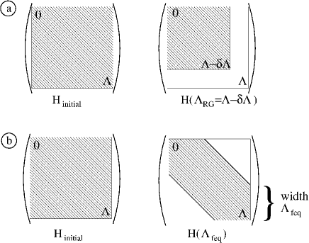
However, one important conceptual difference between these two approaches is that the flow equation approach retains all states in the Hilbert space but decouples them, while the conventional scaling approach actually eliminates high–energy states. If one only focuses on the low–energy physics in an equilibrium problem, this difference is unimportant and the flow equation approach is consistent with the conventional RG–flow with the identification (explicit examples for this observation can be found in Ref. Kehrein_SG ; Kehrein_KM ). In a non–equilibrium situation like the Kondo model with voltage bias the difference is, however, more fundamental. Fig. 1 schematically depicts the two schemes once the cutoff is reduced below the scale set by the voltage bias, . In the flow equation framework the Hamiltonian still describes the stationary current flowing across the dot, while scaling around the separate Fermi surfaces of the two leads does not allow for energy–diagonal transport processes across the dot anymore. Therefore a naive application of the conventional scaling approach purports to eliminate scattering processes with small energy–denominators across the dot, which violates the spirit of renormalized perturbation theory. We will later see that it is precisely this point which allows us to understand qualitatively and quantitatively non–equilibrium decoherence in a Hamiltonian framework.
I.2 Outline
This paper is organized as follows. In Sect. II we define the model and briefly review its conventional scaling analysis. In Sect. III.A we first introduce the flow equation method, and then in part III.B apply it to a general Kondo model Hamiltonian with an arbitrary number of leads with or without voltage bias. This is the core part of our calculation. The resulting equations are then analyzed in equilibrium in part III.C, where we reproduce the conventional two–loop –function. In part III.D and III.E we then specialize to the case of interest in this paper; the Kondo model with two leads and voltage bias . Using these flow equations, we work out and analyze the scaling picture of the Kondo model with voltage bias in Sect. IV. Sect. V discusses our results for the spin dynamics in non–equilibrium, which are compared with the well–known equilibrium behavior at nonzero temperature. In particular Sects. V.C and V.D contain the key new results of this work regarding the spin dynamics and the static spin susceptibility in non–equilibrium. A summary of results and conclusions is presented in Sect. VI. Appendix A contains important commutators and normal–ordering results that are frequently needed, and Appendix B contains details of the numerical solution of the flow equations.
II The Kondo Model with Voltage Bias
II.1 Model
We are investigating a quantum dot that can be modelled by a spin–1/2 degree of freedom coupled to conduction electrons in a left () and a right () lead with no external magnetic field
| (1) |
Here label the two leads, are momentum labels, and the chemical potentials are given by . The conduction band electron spin operators are defined by where are the Pauli matrices. The couplings describe the exchange interaction with the localized spin degree of freedom, with for hermiticiy. If the quantum dot can be described by an Anderson impurity model with tunneling rates from the left/right lead, the coupling constants of our effective Kondo model are related by and Glazman99 . We define as the asymmetry parameter of our model. We will derive the scaling equations without making any of the above assumptions so that also more general complex quantum dot structures can be investigated (e.g., in double dot systems the relation is not necessarily fulfilled). We assume a linear dispersion relation leading to a constant conduction band density of states and introduce the dimensionless coupling constants and ( for transport). The band cutoff is denoted by and we are only interested in the universal behavior on energy scales much smaller than .
II.2 Conventional Scaling Analysis
Below we will sum up the results of the conventional scaling analysis for the non–equilibrium Kondo model in the spirit of Fig. 1, that is reminiscent of Anderson’s “poor man’s scaling” in equilibrium Anderson70 . The derivation of the one–loop results is straightforward, see Refs. Glazman99 ; Coleman01 . Upon lowering the cutoff around the two Fermi surfaces, but while still holds, one finds the equilibrium scaling equations
| (2) | |||||
| (3) | |||||
| (4) |
plus third order terms in the coupling constants. Once the cutoff is reduced below the voltage bias, , the strong–coupling scaling of the coupling stops since there is no sharp Fermi surface for transport processes on this scale. Similarly, only the inter–lead scattering processes still contribute to the scaling equations of and
| (5) | |||||
| (6) | |||||
| (7) |
We now assume that the Kondo model can be derived from an underlying Anderson impurity model, and one easily solves the equation for down to the infrared limit Glazman99
| (8) |
where is the Kondo temperature of the equilibrium model (i.e., for ). The IR–coupling (8) determines the current across the dot and a conventional second order Keldysh calculation in the renormalized quantities yields Glazman99 . This leads to perturbative result for the differential conductance valid in the limit
| (9) |
where
| (10) | |||||
is the conductance in the unitarity limit.
Notice that there is no IR–cutoff mechanism for the inter–lead scattering processes in the scaling equations (5–6) for , which therefore yield strong–coupling divergences even for large voltage bias Coleman01 . However, Rosch et al. have pointed out the importance of spin relaxation processes due to the stationary current.Rosch01 Second order perturbation theory in the renormalized quantities yields the decoherence rate
| (11) |
which cuts off the inter–lead strong–coupling flow and eliminates the possibility of two–channel Kondo physics in Kondo dots that can be derived from an underlying Anderson impurity model. The observation that the non–equilibrium Kondo model becomes a weak–coupling problem for has then been exploited to derive a number of physically relevant quantities like the conduction electron -matrix, the non–equilibrium magnetization and the conductance both with and without an external magnetic field.Rosch03 ; Rosch05 ; Rosch04a ; Rosch04b
III Flow Equation Analysis
III.1 Flow Equation Method
The basic idea of the flow equation approach Wegner94 ; Wilson93 ; Kehreinbook is to make a many–particle Hamiltonian increasingly more diagonal through a sequence of infinitesimal unitary transformations. Such a flow can be generated by the differential equation
| (12) |
with some suitable antihermitean generator ; Eq. (12) then generates a one–parameter family of unitarily equivalent Hamiltonians . We set as the initial Hamiltonian and want to be the final diagonal Hamiltonian. In order to generate a stable expansion it is of fundamental importance to properly deal with energy–scale separation during the flow, similar to conventional scaling approaches. For small (initial phase of the flow) we will decouple modes with large energy differences, while later for large flow parameter we will deal with increasingly more energy–diagonal processes. This sequence of transformations is generically generated by the “canonical” generator suggested by Wegner Wegner94
| (13) |
where is the diagonal part of the Hamiltonian and its interaction part. The flow parameter then has the dimension (Energy)-2, and is the flow equation energy scale that expresses how energy–diagonal the Hamiltonian has become. Interaction matrix elements with energy transfer are eliminated in , while processes with are still retained. We will use the notation with or interchangeably.
The flow equation approach has been successfully applied to numerous equilibrium many–body problems, like dissipative quantum systems Kehrein96 ; Kleff , the two–dimensional Hubbard model Wegner_Hubbard , low–dimensional spin systems Uhrig , and strong–coupling models like the sine–Gordon model Kehrein_SG or the Kondo model Kehrein_KM ; Garst . Due to its intrinsic energy scale separation the flow equation method generates the same IR–scaling flow as conventional renormalization group methods, with the identification . Notice that in certain strong–coupling problems Kehrein_SG ; Kehrein_KM the flow equation approach even allows a controlled systematic expansion in the strong–coupling phase where conventional scaling leads to a strong–coupling divergence.
The main conceptual difference between flow equations and the conventional scaling approach is that in the flow equation approach the Hilbert space remains unchanged while modes become decoupled, whereas in the scaling approach high–energy modes are successively integrated out, compare Fig. 2. This allows one to evaluate correlation functions on all energy scales within the flow equation framework Kehrein96 ; Kehrein_KM , however, for non–equilibrium problems this conceptual difference will turn out to be even more fundamental as we will see later (compare also Fig. 1). Applications of the flow equation approach to non–equilibrium initial state problems have been discussed in Refs. LobaskinKehrein ; HacklKehrein ; MoeckelKehrein . In the sequel, we will explain in detail the flow equation analysis of the stationary non–equilibrium problem provided by the Kondo model with voltage bias.
III.2 Kondo Model
For an interacting many–body problem like the Kondo Hamiltonian (1) the flow equation approach generates higher and higher–order interaction terms in the commutators (12) and (13). Similar to a conventional scaling analysis, the flow therefore needs to be approximated by an expansion in a suitable expansion parameter that remains sufficiently small during the entire flow. In our problem we will use the running coupling constants as our expansion parameters Note_expparameters and perform a consistent systematic expansion in orders of . No further input except this systematic expansion is required to find both coherent and decoherence effects in our non–equilibrium problem in a systematic controlled expansion. Since we are performing unitary transformations (12) which do not explicitly depend on the ground state of the system (though implicitly as we will see below), it is actually advantageous to first derive the differential flow equations for a general Kondo Hamiltonian with couplings to some arbitrary number of leads (with arbitrary chemical potentials). We introduce a general index labelling the conduction band electrons and write
| (14) |
with for hermiticity. This will allow us to study both the equilibrium model without voltage bias and the non–equilibrium model on the same footing. In the equilibrium model there is only one lead, therefore with electron momentum , whereas in the Kondo model with voltage bias the label is a multi–index labelling both lead left/right and electron momentum, with .
III.2.1 and Generator
During the flow equation procedure new interaction terms are generated that are not present in the initial Hamiltonian (14). We will neglect the newly generated normal–ordered terms in and higher in , which can only affect our scaling equations for the couplings in order and higher (since the commutator (12) always increases the order by at least one). We will later see that this order of the flow equation calculation is the minimum order necessary to obtain a controlled expansion in the sense that the flowing coupling constants remain finite for . Higher order calculations beyond our present work can be understood as corrections to the results presented here.
Within our order of the calculation, the flowing Hamiltonian can be parametrized as
where will turn out to be the only newly generated term in . It obeys for hermiticity and initially . In (III.2.1) denotes normal–ordering with respect to the ground state of the system without Kondo impurity. We use the normal–ordering procedure as introduced in Ref. Wegner94 (for more details see the appendix). Notice that we do not need to explicitly normal–order the term proportional to in (III.2.1) since it automatically appears in its normal–ordered form.
The generator of the infinitesimal unitary transformations is given by (13) where the diagonal part of is the conduction band kinetic energy . This leads to
| (16) | |||||
where
| (17) | |||||
| (18) |
Here and in the sequel we will usually suppress the explicit –dependence of all parameters and coupling constants in our notation.
III.2.2 Terms in and
In order to work out the unitary flow of the Hamiltonian (12) we now need to calculate the commutator . This is the main calculational problem of the flow equation approach. For the current problem we will now proceed order by order in the coupling constant with this calculation.
Let us first evaluate . This is straightforward and leads to
Next we need to find . We first identify its contributions in order , which can only come from
| (20) |
The basic commutator is worked out in the appendix and given in (A). Inserting it in (20) yields
plus an uninteresting constant that does not contribute to the further flow. Here we have defined the expectation value with respect to the non–interacting ground state
| (22) |
which is just the occupation number. No summation over is implied in this definition.
Comparing coefficients in (III.2.1), (III.2.2) and (III.2.2) we find the following differential flow equations
From (III.2.2) one would conclude that a new term
| (25) |
is generated in the Hamiltonian that has not been included so far
| (26) |
However, we will see below that this contribution vanishes identically due to symmetry reasons (in fact, it only appears in ).
III.2.3 Terms in
Our goal is to derive the –function of the Kondo model up to two–loop order within the flow equation framework. This implies that we need to calculate the terms in order that contribute to the differential equation (III.2.2) for . Notice that our differential equation for generates this term (which is not present for ) in order . Also notice that we do not need to calculate its –contribution because this can only feed back into the differential equation for in . We are therefore left with identifying the terms with structure in the normal–ordered commutators
and
| (28) | |||||
We can combine these two contributions into
| (29) | |||||
The commutator is worked out in the appendix and given in (A). We only need the contribution with structure and inserting yields
We have now derived all the necessary terms to write down the flow equations to the desired order.
III.2.4 Flow Equations
We include the term (III.2.3) in the differential equation (III.2.2) and find the following set of flow equations that completely determine the flow of the Hamiltonian up to the resp. order in
In order to complete our analysis we finally need to show that the terms from (25) indeed vanish to the required order. This is straightforward by solving (III.2.4) in linear order
| (33) |
and inserting in (26)
Since we assume a linear dispersion relation and initial coupling constants that are constant (at least in the low–energy limit) we only need to know
| (35) |
which holds up to possible band edge effects that do no influence the universal low–energy physics for . Therefore
| (36) |
and the –terms do not influence the flow equations (III.2.4) and (III.2.4) in the orders that we are interested in. In fact, a more detailed analysis shows that even the –terms on the rhs of (36) vanish; the first nonvanishing contributions arise in order .
Eqs. (III.2.4) and (III.2.4) constitute the main computational results of this paper and will now be analyzed in various settings. Notice that they apply for a general spin–1/2 multi–lead Kondo model where we did not yet have to specify whether the system is equilibrium or not. The derivation of these equations followed from a straightforward application of the canonical flow equation framework as an expansion in powers of the flowing coupling constants. Also notice that the linear terms in (III.2.4) and (III.2.4) generate the canonical exponential decay of the coupling constants (33) that make the Hamiltonian increasingly diagonal in energy space (see Fig. 2) with the identification .
III.3 Equilibrium Model
As a consistency check and in order to gain some insight into the system of flow equations we now first analyze the equilibrium Kondo model at zero temperature . Here the index labelling the conduction band electrons in (14) only consists of the electron momentum and we have one exchange coupling . We use the following approximate parametrization of the running couplings as a function of
| (37) |
where is determined from the flow in the IR–limit (we choose ). This parametrization is asymptotically correct in the IR–limit and we can identify with the dimensionless running coupling constant of the conventional scaling approach.
Inserting the parametrization (37) into the flow equation (III.2.4) for
| (38) | |||||
where we have insert the zero temperature occupation numbers
| (39) |
Eq. (38) is integrated starting from where is the conduction band width (UV–cutoff). We also need to the flow of the –terms that are initially not present in the Hamiltonian but generated during the flow: from (III.2.4) we deduce
| (40) | |||||
Eq. (III.3) can be solved easily
| (42) |
From the scaling equation in second order for one obtains the well–known slow logarithmic increase during the flow, therefore the integral in (42) is dominated by large values of and one can write
| (43) |
Putting everything together in (38) and performing the remaining integrations we obtain
| (44) |
In terms of the scaling parameter with dimension energy one can alternatively write
| (45) |
with the correct equilibrium –function to two–loop order Hewson
| (46) |
As expected for the equilibrium model it therefore makes no difference whether one derives the IR–behavior with respect to the conventional scaling parameter or the flow equation scaling parameter (see Fig. 2). In the next section we will explore how these results change in the non–equilibrium situation.
III.4 Non–Equilibrium Model (general parameters)
For the non–equilibrium setting with voltage bias between the left and right lead the label in (14) is a multi–index labelling both left/right lead () and electron momentum . We choose the Fermi energy of the left lead to be and of the right lead to be , therefore we have a current flowing from left to right. For now we will only look at zero temperature .
III.5 Non–Equilibrium Model ()
Eqs. (III.4) and (III.4) can be simplified considerably if the Kondo model can be derived from an underlying Anderson single impurity model. As explained in Sect. II.1, the coupling constants then fulfill the relations and . Notice that the impurity physics is invariant under the exchange since this just amounts to an exchange of the two leads. One can verify easily that the impurity spin only couples to the following linear combination of left and right lead fermion operators
| (50) |
which obey the usual anticommuation relations . The flowing Hamiltonian then takes the form
with the conduction band spin operators defined for the -operators. Eqs. (III.4) and (III.4) simplify to the following form where the external leads do not appear explicitly:
Here we have the initial condition and the zero temperature Fermi distribution function for the -operators
| (54) | |||||
| (58) |
In the sequel we will restrict ourselves to the analysis of (III.5) and (III.5), that is we only investigate a Kondo model that can be realized from an underlying single Anderson impurity model.
IV Scaling Picture of the Kondo Model with Voltage Bias
IV.1 IR–parametrization
Eqs. (III.5) and (III.5) contain the full information about the Hamiltonian flow to the resp. order in the coupling constant. We will analyze these equations both numerically and analytically to understand the scaling behavior of the non–equilibrium Kondo model. In order to get some first insights, we first perform an analytical analysis that is based on some additional approximations. However, we will later see that these approximations are justified with very good accuracy by comparison with the exact numerical solution.
The flow equation differential equations are connected with conventional scaling equations by using an approximation of the following form
| (59) |
which parametrizes the couplings in terms of the dimensionless running coupling constants on an averaged energy scale . (In fact one can choose any energy in with excellent accuracy.) This ansatz solves the linear part of the flow equation (III.5) and allows us to perform the summations over in closed form. One finds
In the cubic term a whole range of values contributes to the integral where the product of the Fermi functions is nonzero. Again with very good accuracy we can replace the couplings under the integral by an average over the window that is responsible for transport,
| (61) |
The integrals over and can then be performed in closed form and one arrives at the following differential equation
We first use this to derive a closed equation for from (61) by averaging over
Of particular importance are also the running coupling constants at the left and right Fermi surfaces
| (64) |
which will turn out to be relevant for the behavior of the quasiparticle resonances (Kondo peaks) and which determine the phase diagram since they correspond to extremal values of as a function of (see Sect. IV.5). Their flow equations follow immediately from (IV.1):
The three differential equations (IV.1), (IV.1) and (IV.1) are one of the key results of this work and allow us to describe and understand the scaling behavior of the non–equilibrium Kondo model.footnote_us
IV.2 Scaling Analysis
We will first analyze (IV.1), (IV.1) and (IV.1) in the initial phase of the flow where . As expected, all three differential equations coincide and one finds for :
| (67) |
Here we have used the approximation , which holds plus correction terms in higher order due to the slow logarithmic flow of . The initial behavior of the running coupling constants is therefore determined by the equilibrium -function (46) as expected. With our initial condition this also agrees exactly with the scaling equations (4) from the analysis of Kaminski et al.Glazman99 (with the identification ).
Once the flow parameter is smaller than the voltage bias, , the scaling equations take a different structure. The effective transport coupling obeys
| (68) |
and the couplings at the left and right Fermi surfaces, resp.,
One notices that the strong-coupling growth of the average transport coupling stops when due to the energy difference of the left and right Fermi surfaces. On the other hand, the couplings at the left and right Fermi surfaces, and , still exhibit the typical Kondoesque strong-coupling behavior in quadratic order on the rhs of (IV.2) and (IV.2). This reflects the inter-lead scattering processes from the left lead back into the left lead, or likewise for the right lead: such processes still see a sharp Fermi surface for all . It is this obervation that has led to the prediction of 2-channel Kondo physics in the Kondo model with voltage bias based on a 1-loop calculation Coleman01 .
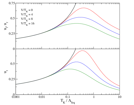
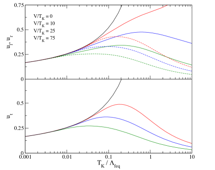
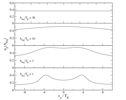
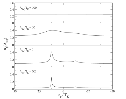
However, different from the experience in equilibrium models the third order terms in (IV.2) and (IV.2) can become more important than the second order terms even for small coupling constants: this is due to the more strongly growing terms as compared to the conventional behavior in quadratic order in the infrared limit . Since the third order term has a positive sign, it counteracts the second order term and can avoid the strong-coupling divergence. Figs. 3 and 4 show the numerical solution of (IV.1), (IV.1) and (IV.1) for symmetric () and asymmetric Kondo dots (). One can see that indeed all couplings remain finite for sufficiently large voltage bias which shows that there is no 2-channel strong-coupling divergence.
Before proceeding with analyzing the resulting phase diagram in more detail, we will first get some more analytical insights into the solution of the scaling equations. The solution of (68) is straightforward
| (71) |
Here
| (72) |
where is the running coupling constant on the scale (since we can safely neglect in the weak-coupling regime). From the solution of (67) we then find
| (73) |
with the Kondo temperature defined from the equilibrium model
| (74) |
In order to understand the implication of the flow of on and it is convenient to first rewrite (IV.2) and (IV.2) in the following equivalent form:
| (75) | |||||
| (76) |
Since
| (77) |
this implies
| (78) | |||||
| (79) |
These equations show a remarkable transmutation of the third order terms in the running coupling constant into linear terms once . This transmutation is possible due to the -terms in (IV.2) and (IV.2) (or, equivalently, due to the -terms in (IV.1) and (IV.1) as opposed to the equilibrium -terms). For these linear order terms are negligible and exhibit typical Kondoesque strong-coupling scaling. In the later phase of the flow the couplings become small again with if they are not already too large on the scale .
Let us analyze the meaning of this scale . We have already quoted the result from Kaminski et al.Glazman99 that for the current is to leading order given by (9)
| (80) |
From (72) we can see that with a propotionality factor independent of , and . It is therefore natural to associate with the spin decoherence rate generated by the shot noise proportional to the current. The third order terms in the scaling equations therefore describe spin decoherence due to the non–equilibrium current that cuts off the strong-coupling behavior of the inter-lead scattering processes. This observation in our Hamiltonian scaling framework is in agreement with the work by Rosch et al.Rosch04b that such non–equilibrium decoherence processes eliminate the 2-channel strong-coupling divergence in the non–equilibrium Kondo model with .
We will next use the flow equation analysis to study quantitatively the interplay between coherent (equilibrium) strong-coupling processes and decoherence generated by the non–equilibrium current in a systematic expansion in terms of renormalized parameters. Before proceeding along these lines, it is worthwile to point out that decoherence acts differently from temperature in the Kondo scaling equations: Decoherence and strong-coupling physics are in competition in (78) and (79), whereas nonzero temperature already eliminates the strong-coupling term itself, e.g.
| (81) |
for the equilibrium Kondo model (37) in both the conventional scaling and the flow equation approach. We would also like to mention the important question of how one can understand within the flow equation framework that the third order terms in the scaling equations are really associated with spin decoherence. We will postpone the answer to this question to the discussion of the dynamic spin correlation function later in Sect. V.3, where we will work out this correspondence in detail.
IV.3 Weak– and Strong–Coupling Regime
From the scaling equation for , and we can now determine the scaling behavior of the non–equilibrium Kondo model: that is we determine the regions in the parameter space where all coupling constants remain small (weak-coupling regime) or where at least one the coupling constants becomes large (strong-coupling regime). Since only and can continue to grow below according to (78) and (79) (as opposed to ), these regions are determined by the behavior of for , or by the behavior of for . Because of the trivial exchange symmetry , we can focus on below without loss of generality.
From (78) we can deduce an (approximate) condition for remaining small during the entire flow
| (82) |
In the notation of the original Kondo Hamiltonian (1) this is equivalent to the inter-lead scattering processes being not too large on the scale
| (83) |
We can approximately rewrite this condition in terms of renormalized quantities by explicitly integrating up the quadratic part of (IV.2). One finds
| (84) |
leading to
| (85) |
Comparison with the numerical solution below shows that (85) can be used as an approxiate condition for the weak-coupling regime for . Before proceeding with the numerical solution of the full differential equation for , one can deduce some important analytical insights from (85): the “critical” value of the voltage bias increases for increasing values of the asymmetry . For larger values of this is due to the fact that decoherence is proportional to the current, which is suppressed for asymmetric coupling to the leads: is maximum for . The third term on the lhs of (85) thus reflects the -dependence of the unitarity limit of the conductance in (10).
The above (approximate) analytical results are confirmed by the exact numerical solution of the full differential equations (IV.1), (IV.1) and (IV.1) for the running couplings and . The definition of “strong-coupling regime” versus “weak-coupling regime” is necessarily not unique since we expect a smooth crossover between these regimes. The definition used in our analysis is that in the weak-coupling regime the couplings and remain smaller than 0.75 during the entire flow, whereas in the strong-coupling regime at least one these coupling becomes larger than 0.75. Choosing a somehow different value than 0.75 (e.g. using 0.5 or 1.0 instead) does actually hardly change the crossover line. The actual value of 0.75 is motivated by the observation that then the -matrix reaches the unitarity limit at the resp. Fermi surface in renormalized second order perturbation theory. This indicates the breakdown of our perturbative expansion in the running coupling constant and therefore limits the region where our method is reliable. The numerical results for this crossover line between strong-coupling and weak-coupling regime are depicted in Fig. 5.
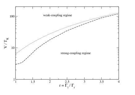
Fig. 5 shows that the strong-coupling regime extends to remarkably large values of the voltage bias for asymmetric Kondo dots (as we have already qualitatively deduced from (85)). By comparison with the flow diagrams in Figs. 3 and 4 we can see that while there is no 2-channel Kondo physics (in the sense of a 2-channel strong-coupling divergence), the crossover to the strong-coupling regime is essentially given by 1-channel Kondo physics for asymmetric Kondo dots: the couplings at the more strongly coupled Fermi surface dominate the Kondo impurity physics.
It should be emphasized again that one expects a smooth crossover between weak-coupling and strong-coupling regimes. While this issue cannot be definitely answered using the weak–coupling tools here, there is no physical reason to expect anything else than a smooth crossover. Notice that for the equilibrium Kondo model at finite temperature we do know that there is a smooth crossover between weak– and strong–coupling regimes. In this context the question arises what physical properties actually distinguish the strong-coupling regime from the weak-coupling regime. We will address this question in detail later when we discuss the behavior of observables: suitable observables behave quantitatively different in these regimes and make the weak-coupling vs. strong-coupling distinction both useful and relevant for the interpretation of experiments. For example in the strong-coupling regime the local density of states remains nearly pinned to its Friedel value at the more strongly coupled Fermi surface, and it only decays once the voltage bias is well into the weak-coupling regime.
IV.4 Expansion Schemes and Higher Orders
We have already mentioned the remarkable transmutation of a third order term in the running coupling constant into a linear term, compare e.g. (IV.2) and (78) for . Decoherence therefore essentially makes the running coupling irrelevant with a canonical scaling dimension for . This teaches an important lesson regarding the well-established notion that higher order terms in the running coupling constant cannot change the results of lower order calculations qualitatively if the running coupling constant remains sufficiently small during the flow (i.e., in the weak-coupling regime). It was exactly this observation which eliminated the possibility of 2-channel Kondo physics due to diverging inter-lead scattering processes.
The technical reason for the transmutation in our non–equilibrium model is the existence of the dimensionful parameter voltage bias , which allows terms like alongside the conventional -terms in the scaling equations (68), (IV.2) and (IV.2). Therefore the possibility of such a transmutation always arises whenever we have dimensionful parameter in a scaling problem, which should be of importance also for analyzing other problems and interpreting the results of lower order calculations. The unavoidable general conclusion is that the expansion order by order in the running coupling constant is not a systematic expansion anymore, unless we can show that no such “transmutation” occurs and changes the results. Notice that for example the equilibrium Kondo model at finite temperature contains the dimensionful parameter temperature , which in fact also leads to transmutation in its third order terms.footnote_finiteT However, already the second order term loses its strong-coupling behavior at sufficiently large temperature according to (81), and therefore no qualitative changes occur due to the third order terms.
It is worthwile to mention again the conceptual difference between the flow equation framework and the conventional scaling analysis around the two Fermi surfaces, compare Fig. 1. For the scaled Hamiltonian has no “knowledge” of the energy scale voltage bias anymore and therefore cannot generate the -terms in third order (2-loop order). On the other hand, the flow equation Hamiltonian still contains all sufficiently energy diagonal scattering processes for (compare Fig. 2), and therefore “knows” about the energy voltage bias because this is the energy window where scattering processes contributing to the current are possible between the left and the right lead. It is exactly this observation which leads to the -terms in the flow equation scaling equations.
In this context one should also address the effect of higher order terms in the flow equation scaling equations. One can verify that the most IR-singular behavior in fourth order is , which is therefore smaller than the third order terms in (68-IV.2) in the weak-coupling regime. In fifth order it seems possible to have contributions that modify the -proportionality factor in our result for the relaxation rate (72), however, they cannot change the structure of (78) or (79). More quantitative results would be a formidable task equivalent to a 4-loop calculation. These observations indicate that the third order calculation presented here should give reliable quantitative results in the entire non–equilibrium weak-coupling regime.
IV.5 Numerical Solution
In the previous sections we have obtained analytical insights into the competition of decoherence and strong-coupling behavior in the non–equilibrium Kondo model. In order to do this we have used various approximations starting from the full set of flow equations (III.5) and (III.5). More accurate results, which also allow us to check the accuracy of the approximations leading to (68-IV.2), can be obtained by solving the full systems of differential equations. These solutions will also be important for obtaining quantitative results for the behavior of dynamical quantities later in Sect. V. The numerical effort for solving (III.5) and (III.5) scales with , where is the number of band states taken into account for the numerical solution: details of the implementation of the numerics are contained in Appendix B.
Figs. 6 and 7 depict the flow of the coupling constants for a symmetric and an asymmetric Kondo dot in the weak-coupling regime. One observes the buildup of strong-coupling behavior at the left and right Fermi surface, followed by decoherence effects that lead to a decay of the coupling constants. In Fig. 7 one can also notice the asymmetry in the buildup of the resonances at the two Fermi surfaces due to the stronger effect of decoherence at the more weakly coupled lead.
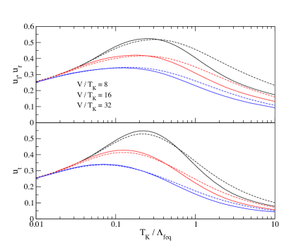
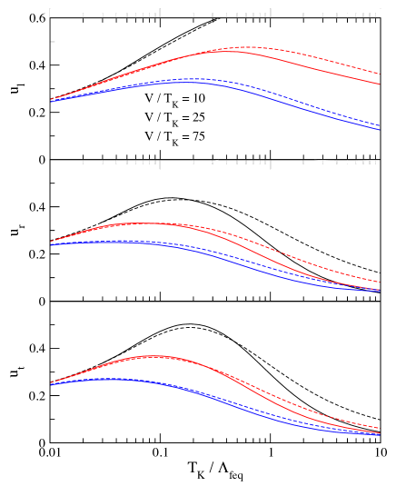
Figs. 8 and 9 shows a comparison of the flow of the coupling constants and from the full numerical solution with the solution of (IV.1), (IV.1) and (IV.1). One can see that our approximations in going from differential equations to just 3 differential equations were very accurate: the resp. solutions agree very well. This agreement is somehow obvious in the initial phase of the flow where the voltage bias plays no role. Therefore one can safely start the full numerical solution at and not waste computer time with larger values of the initial cutoff. The curves agree very well until one reaches the decoherence scale (maximum of the coupling constants), which was important for determining the phase diagram. The small absolute differences at the decoherence scale between the full numerical solution and the analytical approximation get somehow amplified if one looks at the relative error in the later phase of the flow. This will, however, anyway turn out to be unimportant for the evaluation of observables (which are essentially determined by the absolute values of the coupling constants at the decoherence scale). In general one can notice from Figs. 8 and 9 that the accuracy of our analytical approximations (IV.1), (IV.1) and (IV.1) becomes increasingly better if the coupling constants remain small during the flow, that is for larger values of the voltage bias . These obsersations therefore justify a posteriori our previous analytical analysis based on (IV.1), (IV.1) and (IV.1).
V Observables
V.1 Observables in the Flow Equation Framework
The evaluation of dynamical quantities like correlation functions within the flow equation framework is rather different from conventional many-body techniques. The key observation is that while the time evolution becomes trivial in the diagonal basis for , the structure of observables can be very complicated in this basis.Kehreinbook In order to use the time evolution with respect to the diagonal Hamiltonian , one first needs to transform an observable with the same unitary transformations as the Hamiltonian itself (12)
| (86) |
where is the operator in the original basis. Once has found , it becomes easy to work out its equilibrium correlation functions: We are for example interested in
| (87) | |||||
where is the interacting ground state of the system. We denote the unitary transformation that connects the initial with the final basis with , therefore
where we have introduced the notation that designates an operator in the transformed basis. One can (at least formally) construct from (12) in the following way:
| (88) |
Here denotes -ordering in the same way as the usual time-ordering: the generator with the largest is commuted all the way to the left, next comes the second largest, etc. Next one inserts identities everywhere in (87) and arrives at
| (89) |
A key observation is that is just the ground state of the diagonal Hamiltonian , which is therefore trivial to write down (depending on the system for example just the vacuum, the noninteracting Fermi sea, etc.)
| (90) |
The evaluation of equilibrium correlation functions therefore reduces to
| (91) |
Since it is usually straighforward to solve the Heisenberg equations of motion for an operator with respect to the diagonal Hamiltonian , this equation has been used as the starting point for the evaluation of correlation functions in various models like the spin-boson modelKehrein96 ; Kleff , the Kondo modelKehrein_KM , etc. Before proceeding along the same lines we first need to reconsider the changes in this derivation for a non–equilibrium model like the Kondo model with voltage bias.
The fundamental difference from the equilibrium situation is that now we are not interested in evaluating observables in the ground state. Rather, the relevant question is the behavior of observables in the steady state that evolves after switching on the coupling between the left and right lead and then waiting long enough. This is also the key idea of the Keldysh approach and in this manner one circumvents the generally unanswered fundamental question on how to construct a non–equilibrium steady state. We follow the same idea here by replacing (87) with its non–equilibrium generalization
| (92) |
where
Here we assume that the thermodynamic limit is always taken before sending the waiting time for the measurement to infinity in (92). Notice that in general could depend on the initial state and in the sequel we will use an initial state that is directly related to the experimental situation: is the ground state of the system when the two leads are not coupled via the Kondo impurity, that is the noninteracting Fermi sea in both the left and right lead separately.
We now use the same unitary transformations as going from (87) to (89)
The additional unitary transformation of the time-evolved operator in the diagonal basis just maps back to the original basis, where the initial state is specified. This forward-backward scheme has also been employed in other models HacklKehrein where one is interested in real time evolution from some given initial state. The backward transformation part of this scheme can be implemented by solving (86) from to : the initial condition at is just the time-evolved operator in the diagonal basis. In order to evaluate (92) from this expression we next need to say something about the explicit transformation behavior of the spin operator in the next subsection.
V.2 Transformation of the Spin Operator
The transformation of the spin operator under the flow equation transformation has already been worked out in Ref.Kehreinbook and we only give the key steps here. One makes the following ansatz for the flowing observable (86):
| (95) |
and derives the flow equations for the coefficients from (86):
| (96) | |||||
Initially , and under the flow one always finds (see Refs.Kehrein96 ; Kehreinbook ). One easily identifies this scale where rapidly drops to 0 by noticing that is initially only generated in order , therefore initially remains nearly constant since its differential equation only generates terms in order . This picture breaks down on the scale where starts to decay algebraically :
-
i)
Nonequilibrium (voltage bias ):
(97) -
ii)
Equilibrium (nonzero temperature):
(98)
Notice that these energy scales are identical with the flow scale (72) where the transmutation of the third order terms in the coupling constant into linear terms occurs. At this point it is easy to understand this observation: When becomes small, the spin operator (95) completely decays into its entangled form . In the flow of the Hamiltonian this amounts to transforming the marginally relevant interaction term into the irrelevant -term, . This implies that the flow equations for (77–79) become weak-coupling for as discussed before. In the next section we will identify the energy scale where the decoherence effects become important in the Hamiltonian flow with the width of the zero frequency peak of the correlation function, that is the physical relaxation rate.
V.3 Dynamical Spin Response and Correlation Functions
In the following we will use the shorthand for . From (91) one derives the following expression for the symmetrized spin–spin correlation function in equilibrium at nonzero temperature:
| (99) | |||||
Here is the noninteracting Fermi sea and the finite temperature Fermi-Dirac distribution.
For the symmetrized spin–spin correlation function in the non–equilibrium steady state (92) we need to perform the backtransformation (V.1) of for large . Due to the phases that the matrix elements acquire, one can easily see that integrating (96) back from to only leads to higher order contributions in the flow equations. For large times we can therefore say
| (100) |
This implies for the spin–spin correlation function in the steady state (92)
| (101) | |||||
plus higher order corrections in the running coupling constant. Here we now have to insert the occupation numbers (58) for the problem with voltage bias.
Both the nonzero temperature equilibrium result (99) and the steady state non–equilibrium result (101) have the same structure and can therefore be analyzed together: Fourier transformation yields
| (102) | |||||
where the notation stands for the state with energy . Due to the perturbative nature of the transformation the sum rule
| (103) |
is not fulfilled exactly. For high voltage bias or high temperature this violation is typically only of order one percent, which becomes up to ten percent for voltage bias or temperature of order .
The same calculation for the spin susceptibility
| (104) |
yields the imaginary part of its Fourier transform
| (105) | |||||
The real part follows via a Kramers–Kronig relation, in particular the static spin susceptibility is given by
| (106) |
Notice that the fluctuation–dissipation theoremFlucDiss
| (107) |
is fulfilled exactly in equilibrium. In non-equilibrium the fluctuation-dissipation relation is fulfilled approximately in the zero frequency limit if one inserts an effective temperature motivated by the comparison of (97) and (98):
| (108) |
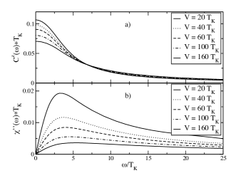
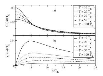
Typical curves for the spin-spin correlation function and the imaginary part of the dynamical spin susceptibility are shown in Fig. 10 for non-equilibrium (for varying voltage bias) and in Fig. 11 for equilibrium (for varying temperature). The spin-spin correlation function is a symmetric function of with a zero frequency peak of width . The imaginary part of the dynamical spin susceptibility is an antisymmetric function of and has its maximum at . An approximate analytical solution of (96) yieldsKehreinbook (see also Ref. Rosch04b ):
| (109) |
| (110) |
Notice that the zero frequency peak of the correlation function is directly related to the flow scale where in the transformation of the spin operator starts to deviate noticeably from 1 since essentially all the spectral weight is contained in the energy interval according to (109). This provides the desired physical interpretation of defined in (72): The energy scale where the Kondo coupling becomes irrelevant can be identified with the spin relaxation rate.
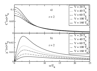
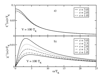
In Fig. 12 we show the spin-spin correlation function and the imaginary part of the dynamical spin susceptibility for asymmetric coupling to the leads with . In Fig. 13 we depict the dependence on the asymmetry paramter at fixed voltage bias. Increasing the asymmetry parameter leads to a smaller decoherence rate since the effective temperature (108) becomes smaller. In agreement with (109) and (110) one therefore notices that mainly the low frequency properties are affected with the maxima of the curves increasing for larger asymmetry.
V.4 Static Spin Susceptibility
One of the most celebrated results of Kondo physics is the behavior of the static spin susceptibility as a function of temperature. This behavior encompasses the screening of the impurity spin via the formation of a Kondo bound state upon lowering temperature. While it is easy to deduce the reduction of the magnetic moment with scaling techniques,
| (111) |
the correct result of a finite nonzero spin susceptiblity at zero temperature, , was first obtained in the seminal application of the numerical renormalization group by Wilson Wilson_NRG . Later the Bethe ansatz BA_thermo ; BA_scales gave the complete analytical solution leading to the high temperature expansion
Likewise, the behavior of the static spin susceptibility as a function of voltage bias is of fundamental importance for understanding non-equilibrium Kondo physics. In the sequel we will focus on the case of zero temperature, zero magnetic field and nonzero voltage bias. The case of nonzero magnetic field will be discussed in a separate publication. The leading order result for for large temperature or large voltage bias was worked out by Parcollet and Hooley Parcollet02 :
| (113) |
This naturally raises the question about the logarithmic corrections to this behavior, similar to the key result (111) of equilibrium Kondo physics. This question has to date only been answered for the leading -corrections, which, however, vanish if the Kondo model can be derived from an underlying Anderson impurity model (see Sect. II.A). The logarithmic terms proportional to have not yet been calculated completely, which means that the current status of the non–equilibrium calculation would miss the finite temperature logarithmic correction in equilibrium (111). More details about these calculations and results can be found in Refs. Rosch03 ; Rosch04a ; Rosch05 based on perturbative RG and Keldysh techniques.
Within the flow equation framework it is straightforward to derive the leading term (113) analytically, but the corrections to it can only be worked out from the full numerical solution of the system of differential equations derived in the previous chapters. Numerical results for the static spin susceptibility obtained in this way via (106) are shown in Figs. 14 and 15.
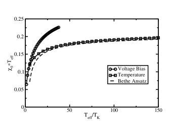
The comparison (Fig. 14) of the Bethe ansatz result (V.4) with the flow equation data points in equilibrium as a function of temperature shows very good agreement for large . This demonstrates that the flow equation calculation presented here contains the leading logarithmic corrections and can address this issue also in non–equilibrium.
Flow equation results for this non–equilibrium spin susceptibility are plotted in Fig. 14 for symmetric coupling to the leads () as a function of the effective temperature , Eq. (108). In this way a direct comparison between equilibrium nonzero temperature and non–equilibrium nonzero voltage bias is possible: Naively, one might expect that not only the zeroth order result (113) can be described by the effective temperature (108), but that this also holds for the logarithmic correction in (111). This is clearly not the case and the logarihmic corrections to contain some genuine non–equilibrium physics.footnote_efftemp Due to numerical limitations it has unfortunately not been possible to go to larger values of the voltage bias to study the full crossover to the analytically known asymptotic behavior .
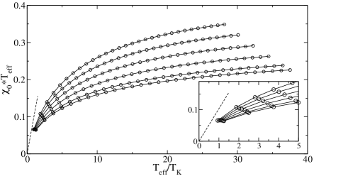
Fig. 15 contains the non–equilibrium static spin susceptibility plotted in the same way for various values of the asymmetry parameter . One can see that the logarithmic corrections get even larger for increasing asymmetry. The values of clearly start to overshoot the asymptotic value for larger asymmetries. As opposed to the equilibrium case, the effective magnetic moment in non–equilibrium first increases upon lowering the voltage bias. This is related to the strong energy-dependence of the running coupling constant in non–equilibrium, see also Figs. 6 and 7. The behavior here is consistent with what one would conjecture based on the analytically known –corrections for a Kondo model that cannot be derived from an underlying Anderson impurity model. In that case the energy–dependence of the couplings becomes even larger than here, eventually reaching two–channel Kondo physics behavior. Likewise, the leading logarithmic corrections to the static spin susceptibility are positive,Rosch03 ; Rosch04a ; Rosch05 which is reminiscent of our results depicted in Fig. 15.
The behavior of the curves for smaller values of the voltage bias in Fig. 15 has to be interpreted with care, since the running coupling constants become larger and therefore the flow equation calculation less reliable. Still, the fact that the curves for different asymmetries converge for smaller voltage bias has a simple physical interpretation: We know that with the Wilson number known exactly from the Bethe ansatz. This result is trivially independent of . This translates into a constant slope in Fig. 15 (dashed line), which all the other curves have to approach in the limit independent of . Notice that our results for the non–equilibrium static spin susceptibility show clear indications of this behavior.
VI Conclusions
This paper has served a twofold purpose. First, we have worked out how the flow equation method can be applied to steady state non–equilibrium impurity models. This was illustrated in detail for the Kondo model with voltage bias. Thereby we have shown how Hamiltonian scaling ideas can be used in non–equilibrium, and how they help to understand the physics qualitatively and also quantitatively. A point of particular importance is the transmutation of marginal terms in the Hamiltonian into irrelevant terms on the energy scale set by the spin relaxation rate, which is generated by the steady state current. This is precisely the effect of decoherence within our Hamiltonian scaling framework.
In addition to these methodological considerations, we have also derived a number of new results for the non–equilibrium spin dynamics in the Kondo model with voltage bias. In this paper we have focussed on the spin dynamics since it contains frequency resolved information about the non–equilibrium steady state (as opposed to the steady state current (9)). For the equilibrium model the spin dynamics is the key to understanding Kondo physics, and therefore the spin dynamics is a very suitable tool to illustrate the differences between equilibrium and non–equilibrium. In particular, we have calculated the static spin susceptibility in non–equilibrium including its logarithmic corrections for a wide range of voltage bias. Although we had to resort to a numerical solution of the flow equations for this purpose, this is an important step since to date an analytical calculation of this leading correction has not been possible (at least for the experimentally most relevant case of a Kondo model that is derived from an underlying Anderson impurity model).
Scaling ideas are one of the key concepts for understanding equilibrium many–body systems. Likewise, we believe that Hamiltonian scaling ideas like the one presented here can play an equally important role for steady state non–equilibrium problems.
Acknowledgements.
We acknowledge valuable discussions with N. Andrei, J. von Delft, A. Mitra, J. Paaske and A. Rosch. This work was supported through SFB/TR 12 of the Deutsche Forschungsgemeinschaft (DFG), the Center for Nanoscience (CeNS) Munich, and the German Excellence Initiative via the Nanosystems Initiative Munich (NIM).Appendix A Commutators and Normal–Ordering
In this Appendix we work out in detail some key commutators that are used throughout our calculations.
1. Commutator
We use the following fundamental property of the spin–1/2 algebra
| (114) |
and insert it into the commutator:
Next we need to normal–order the fermion terms. We introduce the following expectation values with respect to the non–interacting ground state
| (116) | |||||
which are related by because of . No summation over is implied in (116), and the expectation values are obviously independent of due to spin symmetry (no magnetic field). Then
| (117) | |||||
and . For normal–ordering of higher–order fermion terms we follow the prescription of Wegner Wegner94 that not only subtracts the ground state expectation values, but also expectation values with respect to lower–order excited states:
Inserting everything into (A) yields after some straightforward algebra
Normal–ordering in the first term on the rhs of this equation acts on the fermions only
| (120) |
2. Commutator
For notational clarity we use labels instead of
in this section. For the purposes of this paper
we also only need to identify terms with the structure
in the above normal–ordered
commutator. This will simplify our calculation considerably.
Using (114) it is easy to show
The first term does not contain the impurity spin and can therefore not contribute to the terms that we need to extract from the commutator. We can focus on the anticommutator in the second term
In order to yield terms with the structure we need to extract the terms with two contractions (i.e., two –terms) in (A). Similar to (A) one shows
From this expression it is straightforward to show
Combining all the like terms in (A) yields
This gives our desired result by inserting into (A)
Appendix B Numerical Solution
This Appendix contains some details of the numerical solution of the full set of flow equations (III.5) and (III.5). The latter are solved using a standard Runge–Kutta algorithmNR .
One numerical issue arises from the fact that the –couplings in (III.4) depend on four momenta which leads to a large number of differential equations to keep track of. While this is no fundamental problem, it would limit the possible resolution on a standard workstation considerably. However, one can use the following approximation which reduces the complexity to quadratic in the number of momenta and provides an excellent approximation to the full system.
The formal solution of (III.5) is given by
Using this result the flow equations for the running coupling (III.5) in diagonal parametrization
| (127) |
are easily rewritten to the form
| (128) | |||||
where
| (129) |
In the remaining flow equations, for example the transformation of the spin operator, the running coupling is simply replaced by the rhs of (127). The equations above can be easily generalized to the case of general parameters (III.4) and (III.4).
Using diagonal parametrization in the numerical solution effectively reduces the number of differential equations to quadratic in the number of momenta . The runtime is proportional to instead of in the full set. Additionally the stiffness of the differential equations is reduced by removing the exponential decay from the flow of the running coupling. On a standard workstation can be choosen of .
References
- (1) A. Rosch, J. Paaske, and P. Wölfle, Phys. Rev. Lett. 90, 076804 (2003).
- (2) A. Rosch, J. Paaske, J. Kroha, and P. Wölfle, J. Phys. Soc. Jpn. 74, 118 (2005).
- (3) H. Schoeller, Lect. Notes Phys. 544, 137 (2000).
- (4) S. G. Jakobs, V. Meden, and H. Schoeller, Phys. Rev. Lett. 99, 150603 (2007).
- (5) A. Mitra and A. J. Millis, Phys. Rev. B 76, 085342 (2007).
- (6) D. Segal, D. R. Reichman, and A. J. Millis, Phys. Rev. B 76, 195316 (2007).
- (7) S. Kehrein, Phys. Rev. Lett. 95, 056602 (2005).
- (8) A. Hackl and S. Kehrein, Phys. Rev. B 78, 092303 (2008); arXiv:0809.3524
- (9) D. Goldhaber-Gordon, et al., Nature 391, 156 (1998).
- (10) S. M. Cronenwett, T. H. Oosterkamp, and L. P. Kouwenhoven, Science 281, 540 (1998).
- (11) J. Schmid, J. Weis, K. Eberl, and K. von Klitzing, Physica B258, 182 (1998).
- (12) W. G. van der Wiel et al., Science 289, 2105 (2000).
- (13) L. Glazman and M. Raikh, JETP Letters 47, 452 (1988).
- (14) T. Ng and P. A. Lett, Phys. Rev. Lett. 61, 1768 (1988).
- (15) A. Kaminski, Yu. V. Nazarov and L. I. Glazman, Phys. Rev. Lett. 83, 384 (1999); Phys. Rev. B 62, 8154 (2000).
- (16) A. Rosch, J. Kroha, and P. Wölfle, Phys. Rev. Lett. 87, 156802 (2001).
- (17) J. Paaske, A. Rosch, and P. Wölfle, Phys. Rev. B 69, 155330 (2004).
- (18) J. Paaske, A. Rosch, J. Kroha, and P. Wölfle, Phys. Rev. B 70, 155301 (2004).
- (19) F. B. Anders, Phys. Rev. Lett. 101, 066804 (2008).
- (20) E. Boulat, H. Saleur, and P. Schmitteckert, Phys. Rev. Lett. 101, 140601 (2008).
- (21) P. Mehta and N. Andrei, Phys. Rev. Lett. 96, 216802 (2006); P. Mehta, Sung po Chao, and N. Andrei, arXiv:cond-mat/0703426
- (22) M. Moeckel and S. Kehrein, Phys. Rev. Lett. 100, 175702 (2008).
- (23) O. Parcollet and C. Hooley, Phys. Rev. B 66, 085315 (2002).
- (24) For an overview see, e.g., A. C. Hewson, The Kondo Problem to Heavy Fermions (Cambridge Univ. Press, 1993).
- (25) K. G. Wilson, Rev. Mod. Phys. 47, 773 (1975).
- (26) F. Wegner, Ann. Physik (Leipzig) 506, 77 (1994).
- (27) S. Głazek and K. G. Wilson, Phys. Rev. D 48, 5863 (1993); ibid. 49, 4214 (1994).
- (28) S. Kehrein, The Flow Equation Approach to Many-Particle Systems (Springer, Berlin, 2006).
- (29) P. W. Anderson, J. Phys. C 3, 2436 (1970).
- (30) S. Kehrein and A. Mielke, Ann. Physik (Leipzig) 6, 90 (1997).
- (31) S. Kleff, S. Kehrein, and J. von Delft, Phys. Rev. B 70, 014516 (2004).
- (32) I. Grote, E. Körding, and F. Wegner, J. Low Temp. Phys. 126, 1385 (2002); V. Hankevych, I. Grote, and F. Wegner, Phys. Rev. B 66, 094516 (2002).
- (33) C. Knetter, K. P. Schmidt, M. Grüninger, and G. S. Uhrig, Phys. Rev. Lett. 87, 167204 (2001); C. Knetter, K. P. Schmidt, and G. S. Uhrig, Eur. Phys. J. B 36, 525 (2004).
- (34) S. Kehrein, Phys. Rev. Lett. 83, 4914 (1999); Nucl. Phys. B[FS] 592, 512 (2001).
- (35) W. Hofstetter and S. Kehrein, Phys. Rev. B 63, 140402(R) (2001).
- (36) M. Garst et al., Phys. Rev. B 69, 214413 (2004).
- (37) D. Lobaskin and S. Kehrein, Phys. Rev. B 71, 193303 (2005).
- (38) P. Coleman, C. Hooley, and P. Parcollet, Phys. Rev. Lett. 86, 4088 (2001).
- (39) Notice that it is possible to have flow equation expansion parameters different (i.e., more well–behaved) from the running coupling constants, which is the reason why flow equations can yield a controlled expansion even in certain strong–coupling problems Kehrein_SG ; Kehrein_KM .
- (40) The differential equations for correspond to Eqs. (5) and (6) in Ref. Kehrein04, .
- (41) One can work this out easily from (III.2.4) and (III.2.4) with finite temperature Fermi functions .
- (42) V. M. Filyov, A. M. Tzvelik, and P. B. Wiegmann, Physics Letters A 81, 175 (1981).
- (43) N. Andrei and J. H. Lowenstein, Phys. Rev. Lett. 46, 356 (1981).
- (44) See e.g. W. H. Press et al., Numerical Recipes, Third Edition (Cambridge Univ. Press, 2007).
- (45) H. B. Callen and T. A. Welton, Phys. Rev. 83, 34 (1951).
- (46) Another way of saying this is to argue that the effective temperature acquires logarithmic corrections in non–equilibrium. However, one would need to check other observables to verify whether this notion is useful.