Folding Kinetics of Proteins and Cold Denaturation.

Abstract

Folding kinetics of a lattice model of protein is studied. It uses the Random Energy Model for the intrachain couplings and a temperature dependent free energy of solvation derived from a realistic hydration model of apolar solutes. The folding times are computed using Monte Carlo simulations in the region of the phase diagram where the chain occurs in the native structure. These folding times are roughly equals for the temperatures of cold and warm denaturation for a large range of solvent quality. Between these temperatures, the folding times reach maxima and thus, at low temperatures, the kinetics of the chain always speeds up as the temperature is decreased. The study of the conformational space as function of the temperature permits to elucidate this phenomenon. At low temperature, it shows that the activation barriers of the system decrease faster than the temperature as the temperature is decreased. At high temperature, the rate of the barriers over the temperature decreases as the temperature is increased because the height of the barrier is almost constant.

Proteins are very long molecular chains built with given sequences of amino-acids. Under biological solvent conditions, a protein occurs in a unique, native, compact form Anfinsen et al. (1961) and an important goal of theoretical physics is to understand how a chain finds its native structure in a reasonable biological time.

Lattice models, in which the amino acids of the chain are located on the vertices of a two or three-dimensional lattice, are widely used to study protein folding. In the Random Energy Model (REM)Bryngelson and Wolynes (1987); Shakhnovich and Gutin (1990); Dinner et al. (1994); Shakhnovich (1994); Gutin et al. (1995), the couplings between monomers are chosen at random in a Gaussian distribution centered on a negative value. It leads to an energy spectrum where a few (all compact) conformations lye in the bottom discrete part of the spectrum while the large majority of the conformations belongs to a quasi-continuous top part. This spectrum may well mimics that of proteins. However, although REM explains some features of the proteins, it is independent on the temperature and it fails to reproduce a general feature specific to proteins: the cold denaturationKumar et al. (2006); Pastore et al. (2007); Hadi-Alijanvand et al. (2007); Whitten et al. (2007).

The cold denaturation has been first observed by Privalov Privalov and Makhatadze (1989) for Myoglobin which is in its native form between a temperature of warm denaturation $T_{w}$, and a temperature of cold denaturation $T_{c}$. Above $T_{w}$ or below $T_{c}$, the protein is in a denatured state where a lot of conformations are relevant. These temperatures are very sensitive to the pH of the solvent.

Under physiological conditions, the proteins strongly interact with the solvent Kauzmann (1959); Warshel and Lifson (1970); Dill (1990); Premilat and Collet (1997); Collet and Premilat (1996); Frauenfelder et al. (2006) and then any simulation of protein folding must consider a realistic solvent effect on the chain conformations. Recently Collet (2001, 2005), the temperature dependence of the hydrophobic effect has been introduced in the couplings of REM using realistic solvent model based on a qualitative study of the energy spectra of the pure solvent and of the solvent around a monomer Silverstein et al. (1999). As a result, the first phase diagram of protein, where both warm and cold denaturations occur has been calculatedCollet (2001) showing a very good accordance with experimental data. On the other hand, several works has been published on the subject providing alternative models which were able to exhibits theoretically the cold denaturation Hansen et al. (1999); De Los Rios and Caldarelli (2000); Roccatano et al. (2004); Lopez et al. (2008); Patel et al. (2008); Dias et al. (2008)

In this paper, this protein model is first reminded. The different contributions to the effective couplings between monomers are shown as functions of the temperature. This result gives an insight of the modification of conformational space as the temperature is varied. Thus, the kinetic properties of this model are studied in the native region. Folding times are computed versus a solvation parameter and the temperature, using Monte Carlo simulations Metropolis et al. (1953); Chan and Dill (1994). Moreover, the native conformation, the kinetic trap and the transition state are determined by a study of the phase space. Last, the unusual behavior of the folding times at low temperature is elucidated by taking into account the temperature dependence of the free energy of the activation barrier.

I Protein Model

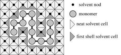
The chain is represented by a string of $N$ beads, (here $N=16$), located on a square two-dimensional lattice. For a given chain conformation, each empty lattice vertice is considered to be a solvent site. It is filled up with four solvent cells pointing towards the four directions (see fig.1). Thus, a solvent cell interacts either with a monomer or with another solvent cell and its thermodynamic properties are determined by the type of this interaction. In such a model, the number of solvent sites and then the number of solvent cells are constant because the chain length is fixed. Hence, the volume of the solvent does not depend on the chain conformation. Moreover, here, a unique parameter $B_{s}$ gives an insight of the solvent quality.

Figure 1: A 12 monomers chain conformation chosen at random.

II Effective Hamiltonian

The system is composed by the chain and a very large number of solvent cells. It is at equilibrium with a bath at temperature $T$ and the probability of occurrence of a chain conformation $m$ in interaction with the solvent is :

$$P_{\rm eq}^{(m)}(B_{s},T)\propto\exp[-{\cal H}_{\rm eff}^{(m)}(B_{s},T)/T]$$

The effective Hamiltonian of conformation $m$ takes into account of all the lattice links and has the following form :

$${\cal H}_{\rm eff}^{(m)}=\underbrace{\sum_{i>j+1}^{N}B_{ij}\ \Delta_{ij}^{(m)}}_{\mbox{intrachain}}+\underbrace{\sum_{i=1}^{N}n_{i}^{(m)}f_{i}(T)}_{\mbox{solvation}}+\underbrace{2n_{s}^{(m)}f_{s}(B_{s},T)}_{\mbox{water-water}}$$

where $B_{ij}$ is the coupling parameter between the monomers $i$ and $j$, chosen at random in a Gaussian distribution centered on 0 with a standard deviation equal to 2 and $\Delta_{ij}^{(m)}$ equals 1 if the monomers $i$ and $j$ are first neighbors on the lattice and 0 otherwise. $f_{i}(T)$ is the free energy of a solvent cell in interaction with monomer $i$ and $f_{s}(B_{s},T)$ is the free energy of a pure solvent cell, $n_{i}^{(m)}$ is the number of links between monomer $i$ and solvent nods and $n_{s}^{(m)}$ is the number of solvent vertices bonds.

The expression of the constant number of total lattice links (equals to $K_{1}$) and the fact that each monomer always creates 4 links leads to write the two conservation equations of the model :

$$\sum_{i}\sum_{j}\frac{1}{2}\Delta_{ij}^{(m)}+\sum_{i}n_{i}^{(m)}+n_{s}^{(m)}=K_{1}$$

$$\sum_{j}\Delta_{ij}^{(m)}+n_{i}^{(m)}=4,\ \ \ ({\rm with}\ \ \ \Delta_{i,i+1}^{(m)}=1)$$

One deduces easily :

$$\left\{\begin{array}[]{l}n_{i}^{(m)}=4-\sum_{j}\Delta_{ij}^{(m)}\\ n_{s}^{(m)}=\sum_{i}\sum_{j}\frac{1}{2}\Delta_{ij}^{(m)}+K_{1}-4N\end{array}\right.$$

Owing to these relations, and after removing the constant terms, the effective Hamiltonian is rewritten as :

$$\begin{array}[]{ll}{\cal H}_{\rm eff}^{(m)}&=\displaystyle\sum_{i}\sum_{j}\left(\frac{1}{2}B_{ij}-f_{i}+f_{s}\right)\Delta_{ij}^{(m)}\\ &=\displaystyle\sum_{i}\sum_{j}\left(\frac{1}{2}B_{ij}-\frac{1}{2}(f_{i}+f_{j})+f_{s}\right)\Delta_{ij}^{(m)}\\ &=\displaystyle\sum_{i}\sum_{j>i}B_{ij}^{\rm eff}(B_{s},T)\Delta_{ij}^{(m)}\end{array}$$

It takes the form of the usual Hamiltonian without solvent effect with effective coupling parameters which now depend on the solvent properties ($B_{s}$) and the temperature :

$$B_{ij}^{\rm eff}(B_{s},T)=B_{ij}-f_{i}(T)-f_{j}(T)+2f_{s}(B_{s},T)\\$$

The model used in this work is that introduced in ref.19. The main difference with that used in ref.18 comes from the factor 2 associated to the free energy of a pure solvent cell in the form of the effective couplings. This function guarantees that the total number of solvent cells (i.e. the volume of the solvent) is a constant whatever the chain conformation. In other words, the creation of an link between monomers and j involves the removing of an interaction between residues i in one hand and j in an another hand with a solvent cell each. These two solvent cells becomes pure solvent.

Obviously, the final form of the effective couplings depends on the solvent model used to calculated $f_{s}$ and $f_{i}$.

III Solvation model

The solvation free energy calculation are based on results of a study of the hydrophobic effect undertaken by Dill and coworkersSilverstein et al. (1999). They used the Mercedes Benz model of water Ben-Naïm (1970) and a simple adaptation of the two-states model of MullerMuller (1990) extended by Lee and GrazianoLee and Graziano (1996) to give a physical picture of the hydrophobic effect in terms of two energy spectra. The first one is associated to the pure solvent and the other one to water molecules in interaction with an apolar solute.

Figure 2: .(a) Energy spectrum of a cell of pure solvent with a unique $N_{s}^{\alpha}$ fold degenerated level of energy $B_{s}$. (b) Energy spectrum of a cell of solvent in interaction with a monomer. $N_{s}$ energy values are draw at random in a Gaussian distribution centered on 0. $B_{i}^{\rm min}$ is specific to each monomer.

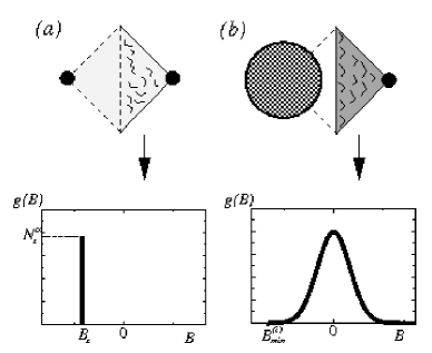
In the spectrum associated to pure solvent, the energy gap between the ground and the low lying exited states is small. Here, these two close energy states are gathered in a unique one of energy $B_{s}$, $N_{s}^{\alpha}$-folds degenerate (see fig. 2(a)). It comes :

$$f_{s}(B_{s},T)=B_{s}-\alpha T\ln N_{s}\qquad{\rm with}\qquad\alpha<1$$

In the other spectrum, the energy gap is larger and the exited state is more degenerate. This picture is reduced further in the spirit of the REM and the spectrum is spread out (see fig.2(b)). For each monomer $i$, $N_{s}$ values of the solvation energies are draw at random in a Gaussian distribution centered on 0 with standard deviation equals 2 and the minimum value of each set of solvation energies, specific to each monomer is determined and noted $B_{i}^{\rm min}$. The free energy of solvent cell in interaction with the monomer $i$ is then :

$$f_{i}(T)=-T\ln\int_{B_{i}^{\rm min}}^{\infty}g(B)\exp(-B/T){\rm d}B$$

where $g(B)$ is the density of energy states, i.e., a Gaussian truncated at $B_{i}^{\rm min}$. Thus, one has :

$$\begin{array}[]{ll}f_{i}(T)&=\displaystyle-T\ln\int_{B_{i}^{\rm min}}^{\infty}\frac{2}{\sqrt{2\pi}}\frac{\exp(-B^{2}/\sigma\sqrt{2})}{{\rm erfc}(B_{i}^{\rm min}/\sigma\sqrt{2})}\ \exp\left(-\frac{B}{T}\right){\rm d}B\\ &=\displaystyle-\frac{\sigma^{2}}{2T}-T\ln\left(N_{s}\frac{{\rm erfc}\left(\frac{B_{i}^{\rm min}}{\sigma\sqrt{2}}+\frac{\sigma\sqrt{2}}{2T}\right)}{{\rm erfc}\left(\frac{B_{i}^{\rm min}}{\sigma\sqrt{2}}\right)}\right)\end{array}$$

.

IV Hydration Results

The solvation parameters used in this work are $\alpha=0.5$, $\sigma=2$ and $N_{s}=10^{5}$.

As it has already pointed out in a another workCollet (2005), by choosing such solvent parameters, one has :

$$B_{ij}=B_{ij}^{\rm eff}-f_{i}-f_{j}+2(B_{s}-\frac{1}{2}T\ln N_{s})$$

Then, using $\alpha=0.5$ in the free energy of the pure solvent is equivalent to the previous workCollet (2001) where the solvent parameter has only been divided by 2.

To well understand the kinetic of folding of the chain present later, we first focus on the different contributions to the effective couplings.

Figure 3: Curves of the different contributions to the effective coupling between the monomers i=1 and j=4 as function of the temperature for several values of the solvent quality. The two temperatures for which the coupling vanishes are shown for $B_{s}=-6.0$.

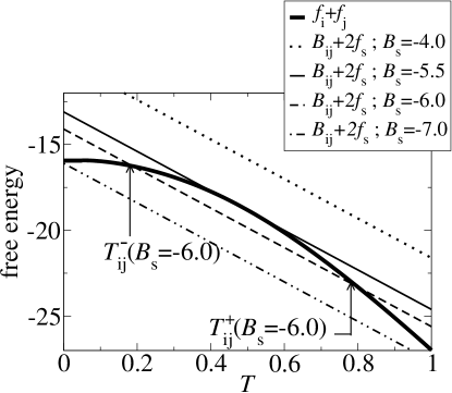
Figure 3 shows that for large values of $B_{s}$, the effective couplings are repulsive, whatever the temperature, because $B_{ij}+2f_{s}>f_{i}+f_{j}$. Thus, this condition corresponds to a good solvent in the sense that the monomers are preferably exposed to the solvent. For small values of $B_{s}$, the couplings are attractive at low temperature, modelling bad solvent condition, and then repulsive at high temperature. Last, for intermediate values of $B_{s}$, the curves of $B_{ij}+2f_{s}$ intersect those of $f_{i}+f_{j}$ twice at two temperatures noted $T_{ij}^{-}$ and $T_{ij}^{+}$. The effective couplings are repulsive for $T<T_{ij}^{-}$ or $T>T_{ij}^{+}$ and attractive for $T_{ij}^{-}<T<T_{ij}^{+}$.

These results show that the free energies of transfer of the residues into water (here $\delta f_{i}=f_{i}-f_{s}$) present maxima for temperatures, depending on $B_{s}$, between $T_{ij}^{-}$ and $T_{ij}^{+}$. This is in good agreement with studies of the temperature dependence of the hydrophobic interaction in protein folding. As an example, first, BaldwinBaldwin (1986) showed from calorimetric data, that the transfer of hydrocarbons in water always exhibits a temperature (denoted as $T_{s}$) for which the entropy of transfer reaches zero ($\Delta S(T_{s})=0$). Using the fundamental thermodynamical relation $\Delta S=-\partial\Delta F/\partial T$, it is clear that the free energy of transfer, $\Delta F$ of the hydrocarbons reaches a maximum at $T_{s}$.

V Protein Thermodynamics

It must be noted that, for given solvent quality and temperature, each intrachain couplings, $B_{ij}$, are different from each other. The functions $f_{i}(T)$ are also specific to each residue because the $B_{i}^{\rm min}$ depend on the monomers. Thus, some couplings are more attractive than other ones. As a results, the ground state of the effective Hamiltonian spectra are non degenerated when the chain is in interaction with a bad quality solvent ($B_{s}\ll 0$) . It corresponds to the native, more maximally compact, conformation of the sequence. The native structure (Nat) is determined by a full enumeration of the conformational space of the chain in interaction with a bad solvent. For several values of $B_{s}$ and $T$, the probability of occurrence of Nat is calculated. If $P_{\rm eq}^{\rm Nat}>1/2$, the chain is in the native phase.

Figure 4: Logarithm of the folding time of the chain versus $B_{s}$ and $T$ in the native region for $-7.0<B_{s}<-5.75$ and $T_{c}(B_{s})<T<T_{w}(B_{s})$.

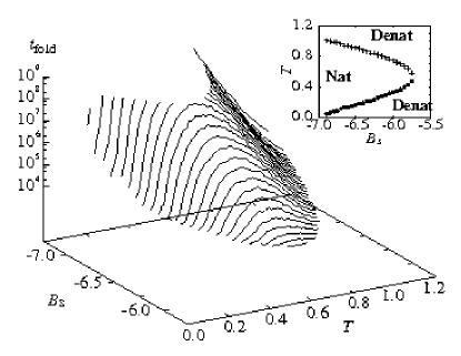
The inset of fig.4 shows the phase diagram of this sequence. For $B_{s}>-5.75$, the chain is always in the denatured phase due to the repulsive couplings and then a lot of different structures are relevant. For $-7.0<B_{s}<-5.75$, the chain occurs in the native state between $T_{c}$ and $T_{w}$ depending on $B_{s}$. Below $T_{c}$ and above $T_{w}$, the chain is denatured. Obviously the cold denaturation, due to the change in the sign of the effective couplings of Nat, occurs for $T_{c}\approx T_{ij}^{-}$. Moreover, with the parameters used in this work, one also has $T_{w}\approx T_{ij}^{+}$. For temperature smaller than $T_{c}$, the couplings are mainly repulsive and then only the numerous chain structures without contact are relevant. Thus, in the cold phase, the probability of occurrence of the Native structure becomes very small. This phase is well denatured because, if it is a glassy phase, the equilibrium probability of occurrence of the native structure would be rather large (and kinetics would be very slow). In the cold denatured phase, the set of the extended structures becomes the relevent sampling of conformations. Hence, kinetics would not converge towards the Native structure but would diffuse freely among the extended structures subset.

At $B_{s}=-7.0$, the couplings are always attractive at low temperature. The cold denaturation disappears and for $B_{s}<-7.0$, only the warm transition remains. A critical point occurs for $B_{s}^{(c)}=-5.75$ and $T^{(c)}=0.53$. At this point, one has $T_{ij}^{-}\approx T_{ij}^{+}$.

VI Protein Kinetics

The folding time, $t_{\rm fold}$, only defined in the native phase, is the mean Monte Carlo steps needed to reach Nat for the first time, averaged over 1000 trajectoriesŠali et al. (1994) . Each trajectory starts with a random conformation and Monte Carlo simulations using the corner flip, the tail and the crankshaft moves used in Chan and Dill (1994); Collet (2003), are performed. The folding times are plotted versus $B_{s}$ and $T$ in fig.4.

For $-5.75>B_{s}>-6.4$, one has $t_{\rm fold}(T_{c})\approx t_{\rm fold}(T_{w})$. That is to say, the folding times are always the same at the temperatures of denaturation in this case (see fig.5).

Figure 5: . Folding times at the temperatures of denaturation as a function of the solvent quality. The filled circle are for the temperature of cold denaturation and the + are for the warm denaturation.

This property may be understood as follow. By definition, the equilibrium probability of occurrence of the native structure equals 1/2 at $T_{c}$ and $T_{w}$. Moreover, it may be seen on the example of fig.6, that, for $Bs=-6.25$, the temperatures of transition are $T_{w}=0.83$ and $T_{c}=0.24$ and the effective Hamiltonian of the native structure for these temperatures are ${\cal H}_{\rm eff}^{\rm Nat}(T_{c})=-4.2$ and ${\cal H}_{\rm eff}^{\rm Nat}(T_{w})=-14.2$ leading to

$${\cal H}_{\rm eff}^{\rm Nat}(T_{c})/T_{c}\approx{\cal H}_{\rm eff}^{\rm Nat}(T_{w})/T_{w}$$

As,

$$\frac{\exp[-{\cal H}_{\rm eff}^{\rm Nat}(T_{c})/T_{c}]}{Z(T_{c})}=\frac{\exp[-{\cal H}_{\rm eff}^{\rm Nat}(T_{w})/T_{w}]}{Z(T_{w})}$$

one deduces the equality of the partition functions, $Z(T_{c})=Z(T_{w})$. Thus, the probability of occurrence of each extended structure, having a zero effective Hamiltonian, is simply one over the partition function and is the same at $T_{c}$ and $T_{w}$. Rationally, to satisfy to the equality of the partition functions, one supposes that the conformational effective Hamiltonians satisfy to ${\cal H}_{\rm eff}^{(m)}(T_{c})/T_{c}\approx{\cal H}_{\rm eff}^{(m)}(T_{w})/T_{w}$ whatever the structure $m$. The configurational spaces where the effective Hamiltonians are roughly linearly scaled by the temperatures may thus be expected for these temperatures. This result holds whatever the solvent quality. To be more precise, the equilibrium probabilities of each structure remains almost constant at the temperatures of denaturation when the solvent quality is varied. As a consequence, the transition rates between two conformations $m$ and $n$, $w(m\rightarrow n,T)=\exp[({\cal H}_{\rm eff}^{(n)}(T)-{\cal H}_{\rm eff}^{(m)}(T))/2T]$, are almost constant at the denaturations temperatures for all $B_{s}>-6.4$, leading to this (quasi) equality of the folding times at $T_{c}$ and $T_{w}$

For $B_{s}\approx-7.0$, the temperature of cold denaturation tends toward 0. The conformational landscape still exhibits a well pronounced effective Hamiltonian minimum for the native structure, but as the temperature becomes very small the transition rates becomes either quasi null or huge. It takes huge amount of time to overcome some local energetic barriers. Thus the folding time tends to infinity at $T_{c}$ because the kinetics is then frozen.

Then, folding time at $T_{c}$ increases rapidly as $B_{s}$ decreases from -6.4 to -7.0.

For each value of $B_{s}$, the folding time goes through a maximum value at a temperature noted $T^{*}(B_{s})$. The region of the curves where $T>T^{*}$, simply confirms that the time needed for a random conformation to reach the native structure increases as the temperature is decreased. However, the behavior of the curves for $T<T^{*}$ is less usual. It corresponds to an increasing of the speed of the kinetics with respect to a decrease of the temperature. This result is not in accordance with standard Monte Carlo simulations and its explanation is given below.

For each temperature, the kinetic trapCieplak et al. (1998) (shown in fig.6) is found using Monte Carlo algorithm by noting the most occurrent conformation during the 1000 trajectories performed to calculated the folding time.

Figure 6: Inset: schematic free energy landscape of a folding pathway from the trap (Tp) to the native (Nat) structure through the transition state (TS) with the activation barrier (arrows) $\Delta F^{\ddagger}(T)={\cal H}_{\rm eff}^{(\rm TS)}-{\cal H}_{\rm eff}^{(\rm Trap)}$. Main: free energy of the native (square), the trap (filled circle) conformations and the transition state (+) versus temperature for $B_{s}=-6.25$. The arrows show some free energy barriers $\Delta F^{\ddagger}(T)$.

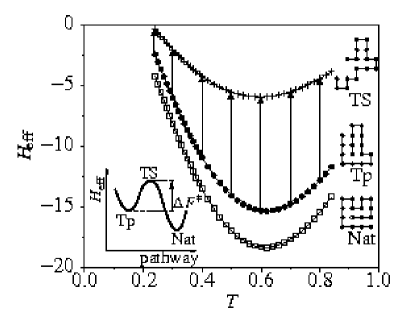
It is observed that the trap do not depend on the temperature. The trap present a great similarity with the native structure. Six contacts among the nine contacts of Nat are observed in trap. Thus, its effective Hamiltonian is very close from that of Nat showing that this structure could be a good candidate for the trap of the system. Second, there is no physical pathway from trap to Nat keeping unbroken the whole set of contacts. That is to say, in a typical trajectory from the trap to Nat, each contact of the trap has to be broken and some of them created again in an other global arrangement. Obviously, they are not simultaneously broken. If it were the case, the trajectories would contain some extended structures without contacts which would have a very great difference of effective Hamiltonian with the trap. Consequently, even step by step, the transition rate for such sub-pathway would be quasi-null. Thus, in more favorable pathways, some contacts are broken while some others are created and the chain walks through local rearrangements toward Nat without reaching any extended conformation. A particular structure of the sequence is the transition state. It is determined by performing a new simulation of 1000 trajectories where the trap is always the first conformation. For each trajectory, the conformation of highest value of the effective Hamiltonian is considered as a possible transition state. The transition state (TS) is the structure with the lowest value of effective Hamiltonian among the sampling of possible transition states collected over the 1000 trajectories (see inset of fig.6). Among all the possible pathways from trap to Nat, those passing through TS are the less energetically costly. One must note that this is not the usual definition of the transition state adopted in the theory of protein folding where the TS is not a unique structure but an ensemble of configurations of highest free energy along the path or paths between unfolded macrostates and the native structure Onuchic et al. (1996). Here, the defintion of the TS is that used in the theory of the simple gaz chemical reactions. Moreover, as explained above, it can be seen that TS has a weak similarity with Nat or with the trap.

The key role of the trap in the folding process is explained as follow. Some trajectories, starting by a random conformations, fall in the trap valley. To leave this structure the chain has to overcome the largest barrier of the system. On the other hand, the trajectories which do not reach the trap valley, walk down the native structure, passing quickly over smaller barriers. Thus, only the trap activation barrier is considered in the folding analysis.

For $B_{s}=-6.25$, the values of the effective Hamiltonian for Nat, the trap and TS are reported on fig.6. The activation barrier between the trap and Nat structures, $\Delta F^{\ddagger}={\cal H}_{\rm eff}^{(\rm TS)}-{\cal H}_{\rm eff}^{(\rm Trap)}$, shown on fig.6, obviously depends on the temperature. For $T>0.60$, $\Delta F^{\ddagger}$ is almost constant whereas it decreases very quickly with the temperature for $T<0.45$. Moreover, the kinetic theory indicates that the time needed to escape from the trap valley is in proportion to $\exp(\Delta F^{\ddagger}/T)$. Figure 7 showed the very sharp decreasing of $\Delta F^{\ddagger}/T$ with respect to a decrease of the temperature for $T>0.45$. One must noted the quasi equality of this last quantity at the temperatures of denaturation.

Figure 7: Logarithm of the folding time (filled square) and $\Delta F^{\ddagger}(T)/T$ (filled circle) versus the temperature for $B_{s}=-6.25$.

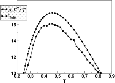
The values of $\Delta F^{\ddagger}/T$ and that of the folding time starting from a random structure, reported in fig.7, present maxima at the temperature, $T_{1}\approx 0.45$. For $T<T_{1}$, the rate $\Delta F^{\ddagger}/T$ decreases as the temperature is decreased because $\Delta F^{\ddagger}$ decreases faster than $T$. For $T>T_{1}$, the rate $\Delta F^{\ddagger}/T$ decreases as the temperature is increased because $\Delta F^{\ddagger}$ is almost constant and, obviously, $1/T$ decreases. As, the folding time is in proportion to $\exp(\Delta F^{\ddagger}(T)/T)$, this result permits to elucidate why the lower the temperature, the faster is the kinetics at low temperature and the higher the temperature, the faster also is the kinetics at high temperature.

VII Conclusion

Our model predicts and explains unusual behavior of the folding times due to the flatness of the conformation space as the temperature decreases towards $T_{c}$. In the native region, far from the denaturation temperatures, $P_{\rm eq}^{\rm Nat}$ tends to 1, leading to a very rough conformational landscape. On the opposite, around $T_{c}$, effective Hamiltonian of all conformations are quasi equal and the free energy landscape is quasi flat. For low temperatures, the difference of effective Hamiltonian between two conformations decreases faster than the temperature. This leveling of the conformational space close to the cold transition leads to a drastic decrease of the free energy barriers of the configurational space leading to an acceleration of the kinetics as the temperature decreases. Last and unfortunately, at the present time, they are no experimental results available for the folding kinetics of proteins at temperatures close to that of cold denaturation. which should be compared to this theoretical prediction.

References

- Anfinsen et al. (1961) C. B. Anfinsen, E. Haber, M. Sela, and W. F.H., Proc. Natl. Acad. Sci. 47, 1309 (1961).
- Bryngelson and Wolynes (1987) J. D. Bryngelson and P. G. Wolynes, Proc. Natl. Acad. Sci. USA 84, 7524 (1987).
- Shakhnovich and Gutin (1990) E. I. Shakhnovich and A. M. Gutin, Nature 346, 773 (1990).
- Dinner et al. (1994) A. Dinner, A. Šali, M. Karplus, and E. Shakhnovich, J. Chem. Phys. 101, 1444 (1994).
- Shakhnovich (1994) E. I. Shakhnovich, Phys. Rev. Lett. 72, 3907 (1994).
- Gutin et al. (1995) A. M. Gutin, V. I. Abkevich, and E. I. Shakhnovich, Proc. Natl. Acad. Sci. USA 92, 1282 (1995).
- Kumar et al. (2006) R. Kumar, A. Prabhu, D. Rao, and A. Bhuyan, J. Mol. Biol. 364, 483 (2006).
- Pastore et al. (2007) A. Pastore, S. Martin, A. Politou, T. Kondapalli, K.C. Stemmler, and P. Temussi, J. Am. Chem. Soc. 129, 5374 (2007).
- Hadi-Alijanvand et al. (2007) H. Hadi-Alijanvand, F. Ahmad, and A. Moosavi-Movahedi, Protein Journal 26, 395 (2007).
- Whitten et al. (2007) S. Whitten, A. Kurtz, M. Pometun, A. Wand, and V. Hilser, Biochemistry 45, 10163 (2007).
- Privalov and Makhatadze (1989) P. L. Privalov and G. I. Makhatadze, J. Mol. Biol. 205, 737 (1989).
- Kauzmann (1959) W. Kauzmann, Adv. Protein Chem. 14, 1 (1959).
- Warshel and Lifson (1970) A. Warshel and S. Lifson, J. Chem. Phys. 53, 582 (1970).
- Dill (1990) K. Dill, Biochemistry 29, 7133 (1990).
- Premilat and Collet (1997) S. Premilat and O. Collet, Europhysics Letters 39, 575 (1997).
- Collet and Premilat (1996) O. Collet and S. Premilat, Journal of Molecular Structure. Theochem 363, 151 (1996).
- Frauenfelder et al. (2006) H. Frauenfelder, P. Fenimore, G. Chen, and B. McMahon, Proc., Natl., Acad., Sci., USA 103, 15469 (2006).
- Collet (2001) O. Collet, Europhys. Letters 53, 93 (2001).
- Collet (2005) O. Collet, Europhys. Letters 72, 301 (2005).
- Silverstein et al. (1999) K. A. T. Silverstein, A. D. J. Haymet, and K. A. Dill, J. Chem. Phys. 111, 8000 (1999).
- Hansen et al. (1999) A. Hansen, M. H. Jensen, K. Sneppen, and G. Zocchi, cond-mat/9905357 (1999).
- De Los Rios and Caldarelli (2000) P. De Los Rios and G. Caldarelli, Phys. Rev. E 62, 8449 (2000).
- Roccatano et al. (2004) D. Roccatano, A. Di Nola, and A. Amadei, J. Phys. Chem. B. 108(18), 5756 (2004).
- Lopez et al. (2008) C. F. Lopez, R. K. Darst, and P. J. Rossky, J. Phys. Chem. B. 112(19), 5961 (2008).
- Patel et al. (2008) B. A. Patel, P. G. Debenedetti, F. H. Stillinger, and P. J. Rossky, J. Chem. Phys. 128, 175102 (2008).
- Dias et al. (2008) C. L. Dias, T. Ala-Nissila, M. Karttunen, I. Vattulainen, and M. Grant, Phys. Rev. Lett. 100, 118101 (2008).
- Metropolis et al. (1953) N. Metropolis, A. W. Rosenbluth, M. N. Rosenbluth, A. H. Teller, and E. Teller, J. Chem. Phys. 21, 1087 (1953).
- Chan and Dill (1994) H. S. Chan and K. A. Dill, J. Chem. Phys. 100, 9238 (1994).
- Ben-Naïm (1970) A. Ben-Naïm, J. Chem. Phys. 54, 3682 (1970).
- Muller (1990) N. Muller, Acc. Chem. Res. 23, 23 (1990).
- Lee and Graziano (1996) B. Lee and G. Graziano, J. Am. Chem. Soc. 118, 5163 (1996).
- Baldwin (1986) R. Baldwin, Proc., Natl., Acad., Sci., USA 83, 8069 (1986).
- Šali et al. (1994) A. Šali, E. Shakhnovich, and M. Karplus, J. Mol. Biol. 235, 1614 (1994).
- Collet (2003) O. Collet, Phys. Rev. E 67, 061912 (2003).
- Cieplak et al. (1998) M. Cieplak, M. Henkel, J. Karbowski, and J. Banavar, Phys. Rev. Lett. 80, 3654 (1998).
- Onuchic et al. (1996) J. Onuchic, D. Socci, Z. Luthey-Schulten, and P. Wolynes, Folding & Design 1, 441 (1996).