Effect of gas flow on electronic transport in a DNA-decorated carbon nanotube

Abstract

We calculate the two-time current correlation function using the experimental data of the current-time characteristics of the Gas-DNA-decorated carbon nanotube field effect transistor. The pattern of the correlation function is a measure of the sensitivity and selectivity of the sensors and suggest that these gas flow sensors may also be used as DNA sequence detectors. The system is modelled by a one-dimensional tight-binding Hamiltonian and we present analytical calculations of quantum electronic transport for the system using the time-dependent nonequilibrium Green’s function formalism and the adiabatic expansion. The zeroth and first order contributions to the current $I^{(0)}(\bar{t})$ and $I^{(1)}(\bar{t})$ are calculated, where $I^{(0)}(\bar{t})$ is the Landauer formula. The formula for the time-dependent current is then used to compare the theoretical results with the experiment.

1 Introduction

Carbon nanotubes (CNTs) [1] have inspired many researchers to investigate and develop CNT-based devices for electronic sensing of various gases and chemical odours [2, 3, 4, 5, 6, 7]. The chemical sensing capabilities of CNT-based devices appear very promising because of their unique structural and electrical properties [1]. However, these devices have a limitation that they can detect only those molecules which bind to them, as some chemical species do not interact with the bare CNTs. Research emphasis to overcome this limitation of CNT-based sensors has led to the development of novel sensing materials and technologies. The sensing capability of CNTs can be improved by their functionalization with certain molecules or polymers [8, 9, 10, 11, 12]. Functionalization of CNT, especially with DNA (DNA-CNT hybrid), has attracted the attention of many experimental [12, 13, 14, 15, 16] and theoretical [17, 18, 19, 20] groups in the past few years. The fascinating DNA-CNT hybrid has led to a vast range of improved and novel applications in nanotube dispersion and sorting [13, 14, 16], and chemical [12] and biological sensing [15]. To realize such applications, a detailed understanding of the fundamental molecular interactions, physical and electronic properties of DNA-CNT hybrids is required. In this connection, theoretical studies have been done on DNA-CNT hybrids [21] to explain their stability [17], DNA sequencing [18], and the interaction of the bases with the CNT [19, 20].

The study of electronic transport properties of DNA functionalized CNT sensors is one of the most active areas of today’s research due to the spectacular combination of molecular and mesoscopic scale phenomena. Electronic transport in these systems is divided into stationary and time-dependent phenomena. Stationary transport for nonequilibrium systems has been studied by many authors [22, 23]. Meir and Wingreen [24] reformulated the ideas given in [22] (and references therein) using the Keldysh approach to study interacting mesoscopic systems, leading to a Landauer formula. Later, Wingreen et al [25] introduced a general formulation for time-dependent transport through mesoscopic structures. Using this formalism a theoretical understanding of experiments [25, 26] has been presented for time-dependent voltages. In this work, we present an analytical treatment of the electronic transport in gas flow over a single-stranded DNA (ss-DNA)-decorated single wall carbon nanotube (SWNT) connected to source (S) and drain (D) contacts maintained at zero gate voltage $V_{g}=0$ V and a fixed bias voltage $V_{b}=100$ mV using a tight-binding model in conjunction with the time-dependent nonequilibrium Green’s function formalism (NEGF) [22]. To our knowledge, there has not been much theoretical work done to study the quantum transport in such a gas sensor and this manuscript is an important contribution in this direction. The choice of this model system is motivated by the experiment [12] that found the current-time characteristics of ss-DNA-decorated SWNT-FET sensors upon odour and air exposures. The SWNTs used in the experiment [12] were all selected to be p-type semiconducting SWNTs with diameters ranging from 1 to 2 nm, but not all the same chirality . For this system, time-dependence arises as a different number of gas molecules flows over and interacts with the DNA-decorated SWNT at each time $\bar{t}$ s for an exposure time of 50 s. This results in the hopping integral and on-site energy being functions of time, and leads to a time-dependent Hamiltonian for the SWNT. Experimentally, the length of the nanotubes varies between 5 and 10 $\rm\mu m$ and electrodes are deposited on the nanotube with a separation of about 1.5 $\rm\mu m$. So only a fraction of the nanotube length is involved in transport. The bare devices do not respond to odours such as dimethyl methylphosphonate (DMMP), 2, 6 dinitrotoluene (DNT), propionic acid (PA), and methanol while for trimethylamine (TMA) the response is weak [12]. The sensor response is observed only when the device is coated with DNA. Since the length of the DNA sequence is of the order of a few nanometers, then the effective length of the SWNT $(L_{eff})$ which contributes to a change in the conductance is of the same order. Therefore, the effective length of the nanotube is assumed to be less than the phase coherence length. Thus, to study quantum transport in gas flow over such nano-structures the time-dependent NEGF formalism is well suited. The characteristic curves show fluctuations in the current response. We calculate these fluctuations in terms of the two-time current correlation function.

2 two-time current correlation function

We begin with the calculation of the two-time current correlation function using the experimental data [12]. The two-time current correlation function $C(\bar{t})$ is defined as

$$C(\bar{t})={\frac{1}{n}\sum_{i=1}^{n}I_{i}(\bar{t})I_{i}(\bar{t}+\delta\bar{t})-\frac{1}{n}\sum_{i=1}^{n}I_{i}(\bar{t})}\times{\frac{1}{n}\sum_{i=1}^{n}I_{i}(\bar{t}+\delta\bar{t})},$$ (1)

where $I_{i}(\bar{t})=I_{i}(\bar{t})/{I_{0}}$ is the normalized source-drain current at time $\bar{t}$ in the $i^{th}$ gas exposure cycle. Let us consider $\delta\bar{t}=1$ s and $n$ is the total number of exposure cycles.

The correlation function calculated here is different from that shown in our previous work [27] equation (2) and for other mesoscopic systems [28] equation (5.57) and [29]. The second terms in equation (2) of [27] and equation (5.57) of [28] are $<I_{i}(t)>^{2}$ and $<g>^{2}$ respectively, where $<\cdots>$ denotes the ensemble average. Instead of $<I_{i}(t)>^{2}$, here we use $\left(\frac{1}{n}\sum_{i=1}^{n}I_{i}(\bar{t})\right)\times\left(\frac{1}{n}\sum_{i=1}^{n}I_{i}(\bar{t}+\delta\bar{t})\right)$, as the average $\frac{1}{n}\sum_{i=1}^{n}I_{i}(\bar{t})$ is different from the average $\frac{1}{n}\sum_{i=1}^{n}I_{i}(\bar{t}+\delta\bar{t})$, because for each $\delta\bar{t}$ there is contribution to the current from another base. In the system (Gas+DNA+SWNT complex), at $\delta\bar{t}=\bar{t}_{1}$ s the gas molecule interacts with a base (say, cytosine) attached to the carbon atom and for the next $\delta\bar{t}$ the gas molecule interacts with another base thymine (say), so for each $\delta\bar{t}$ the current changes as the Gas-DNA-base complex changes upon gas exposure. This is not the case for the usual disordered mesoscopic systems considered in experiments, where both the averages $\frac{1}{n}\sum_{i=1}^{n}I_{i}(\bar{t})$ and $\frac{1}{n}\sum_{i=1}^{n}I_{i}(\bar{t}+\delta\bar{t})$ are the same ([28] equation(5.57) and [29]).

We observe distinct patterns for the different odours and sequences, figure 1. This indicates selective recognition of each odour by the sensors. In particular, the pattern of the correlation function for methanol with sequence 1, figure 1(c), is different from methanol with sequence 2, figure 1(d). This shows that the correlation function is sensitive to different gases and DNA sequences. Hence, the two-time current correlation function is a measure of the sensitivity and selectivity of the DNA-decorated SWNT sensors. The correlation function suggests that these gas flow sensors may also be used as DNA sequence detectors, where the pattern of correlation functions may be used as a benchmark for the particular chemical signal encoded in a DNA sequence. Such an analysis to study the sensor response for gas sensors has never been done before. Figure 1 shows highly fluctuating data, these fluctuations are due to the structure of the DNA sequences as shown in [27].

3 Tight-binding model and nonequilibrium Green’s function

The experiment [12] with gas exposure indicates that the sensor response ($\Delta I/{I_{0}}$) is zero for pristine SWNT, and as DNA is applied on SWNT the sensor response changes. When SWNTs are coated with DNA the bases bind to SWNTs through vdW forces and by forces due to their mutual polarization, which results in a charge transfer from DNA to the SWNT [13, 18, 19, 20]. The gas molecules get adsorbed on SWNTs through vdW forces and/or mutual polarization between the gas molecules and the DNA-SWNT complex [27]. The interaction of gas molecules with DNA-decorated SWNT causes charge redistribution leading to a fractional charge transfer from the Gas-DNA-base complex to the SWNT [27]. This is responsible for the change in sensor current. It is assumed that the charge transfer from the Gas-DNA-base complex to the SWNT is larger than the charge transfer from DNA base to the SWNT, as the net charge transfer from DNA base to the SWNT is found to be small [18]. Since the ss-DNA sequence is a linear chain, and only those nearest-neighbour carbon atoms contribute to the changes in current which interact with the DNA bases, so we model the ss-DNA-decorated SWNT using a one-dimensional tight-binding Hamiltonian for the SWNT, where the electron hops between carbon atoms with different hopping integrals and on-site energies at different times. In our formalism, the effect of gas flow and DNA functionalization in the channel can be modelled by a time-dependent potential. Here, we model the effect by the time-dependent hopping integrals and on-site energy in a self-consistence manner [30].

Now we investigate electronic transport through the model system using the time-dependent NEGF formalism. For this, a tight-binding model of the SWNT and Gas-DNA complex is set up. In this microscopic tight-binding model, there are two approximations: the first approximation is the tight-binding between the carbon atoms of SWNT and the second is the interaction between the carbon atoms of SWNT and Gas-DNA-base complex, where we assume that the carbon atom interacts with the nearest-neighbour DNA base.

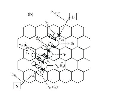
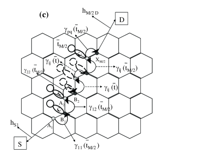
Figure 2: Portion of an unwrapped SWNT. ${\gamma_{ij}(\bar{t})}$ are the hopping integrals indicating hopping between different carbon atoms $A_{i}$ and $B_{i}$ at time $\bar{t}$. Here, $\bar{t}=\bar{t}_{1},\bar{t}_{2},\cdots,\bar{t}_{M/2}$. $\gamma_{0}$ represents the hopping integral in the absence of the gas. $h_{\rm S1}$ represents the coupling between the source contact and the first carbon atom $A_{1}$ while $h_{M/2\rm~{}D}$ is the coupling between the last carbon atom $X_{M/2}$ and the drain contact. The ovals represent the bases cytosine, thymine etc. of DNA sequence 2 while the circles indicate the gas molecules.

Figure 2 shows the schematic diagram of the chosen model system, i.e., Gas-DNA-SWNT sandwiched between S and D contacts. Here, we present a simplified picture of the complex model and its operation. $X_{i}=A_{1}$, $B_{1}$, $A_{2}$, $B_{2}$, $\cdots$ represents the carbon atoms, where $X$ can be A or B, the index $i=1,2,\cdots,(M+1)/2\rm~{}or~{}M/2$ is the number of the carbon atom and $M$ is the total number of carbon atoms. The first and the last carbon atoms, $A_{1}$ and $X_{M/2}$ ($X_{(M+1)/2}$) are connected to S and D. The bases cytosine, thymine etc. of an ss-DNA sequence 2 [12] (shown by ovals) are attached to different carbon atoms and the circle represents the gas molecule. The arrow indicates the path of transmission.

The operational principle of the model is based on the changes in its electrical properties due to DNA bases and gas molecules adsorbed on the SWNT surface. Initially, the DNA sequence is applied on the SWNT, e.g., the cytosine base attaches to the carbon atom $B_{1}$ and thymine base attaches to $A_{2}$ and so on. When the gas is exposed to the sensor for a duration of 50 s, then at time $\bar{t}_{1}$ s the gas molecule interacts with the cytosine base through vdW forces and/or mutual polarization [27]. As a result, the electron hops from the $\pi$ orbital of one carbon atom $A_{1}$ to the neighboring carbon atom $B_{1}$ and the tunnelling of the electron from $A_{1}$ to $B_{1}$ is an elastic process with the corresponding integral referred to as the hopping integral $\gamma_{11}(\bar{t}_{1})$. Then, the electron hops from $B_{1}$ to $A_{2}$ with the hopping integral $\gamma_{12}(\bar{t}_{1})$, and from $A_{2}$ to $B_{2}$ with $\gamma_{22}(\bar{t}_{1})=\gamma_{0}$, where $\gamma_{0}$ is the hopping integral without the gas. Hence, the hopping integrals between other carbon atoms $\gamma_{ij}(\bar{t}_{1})$ are also $\gamma_{0}$, figure 2(a). The indices $i(j)$ =1,2,$\cdots p(q)$ where $p=q=M/2$ for even $M$ and $p={(M-1)}/2$ and $q={(M+1)}/2$ for odd $M$. The timescale of electron transport through the SWNT is far less than the experimental timescale of the gas flow, therefore the electron sees a steady state at $\bar{t}_{1}$ s. Similarly, at $\bar{t}_{2}$ s another gas molecule interacts with the thymine base attached to the carbon atom $A_{2}$, resulting in the hopping integrals $\gamma_{11}(\bar{t}_{2})$, $\gamma_{12}(\bar{t}_{2})$, $\gamma_{22}(\bar{t}_{2})$, and other $\gamma_{ij}(\bar{t}_{2})$=$\gamma_{0}$, figure 2(b). In this case, the electron sees a steady state at $\bar{t}_{2}$ with $\gamma_{ij}(\bar{t}_{2})$ different from $\gamma_{ij}(\bar{t}_{1})$ when the bases interacting with the gas molecules are different. In a similar way at time $\bar{t}_{M/2}$ for even $M$, the time when the gas molecule interacts with the last base of the DNA sequence 2 attached to the carbon atom, the hopping integrals are $\gamma_{11}(\bar{t}_{M/2})$, $\gamma_{12}(\bar{t}_{M/2})$, $\cdots$, $\gamma_{pq}(\bar{t}_{M/2})$, figure 2(c). Hence, we find the hopping integrals as well as the on-site energy change with the time $\bar{t}$ at which the gas molecules trigger the different bases of the DNA sequence attached to the SWNT and depend on the DNA bases, gases, and geometry of attachment of the bases and gases to the SWNT. Because of the time-dependent hopping integral and on-site energy the relevant Green’s functions for the SWNT $(G_{\rm C})$ are also time-dependent.

As the experimental timescale of the gas flow is larger than the time of electron transport inside the SWNT ($\sim 10^{-15}-10^{-17}$s) one can express the leading transport properties of the metal-SWNT-metal system in terms of the Green’s function given by $G(\epsilon,\bar{t})={[\epsilon-H(\bar{t})]}^{-1}$, where $\epsilon=\varepsilon\pm\rmi\eta$ with $\rmi\eta$ an infinitesimal imaginary term and $H(\bar{t})$ is the Hamiltonian at time $\bar{t}$, using the time-dependent NEGF formalism, an adiabatic expansion in the slow time variable $\bar{t}=\frac{t+t{{}^{\prime}}}{2}$ and Fourier transforming with respect to the fast variable $(t-t^{\prime})$ [22, 31]. The time-dependent nonequilibrium retarded and advanced Green’s functions for the SWNT can be derived as $G^{r,a}_{\rm C}(\epsilon,\bar{t})={[{\epsilon}-H_{\rm C}(\bar{t})-{\Sigma}_{\rm S}(\epsilon,\bar{t})-{\Sigma}_{\rm D}(\epsilon,\bar{t})]}^{-1}$, where $\Sigma_{\rm S}(\epsilon,\bar{t})$ = ${h^{\dagger}_{\rm{SC}}}g_{\rm S}(\epsilon,\bar{t}){h_{\rm{SC}}}$ and $\Sigma_{\rm D}(\epsilon,\bar{t})$=${h_{\rm{CD}}}g_{\rm D}(\epsilon,\bar{t}){h^{\dagger}_{\rm{CD}}}$ are the self-energy terms due to metallic contacts, with $g_{\{\rm S,\rm D\}}(\epsilon,\bar{t})=[{\epsilon}-H_{\{\rm S,\rm D\}}(\bar{t})]^{-1}$ the Green’s functions of the contacts. This is done by expanding the Green’s functions up to linear order in the slow variable $\bar{t}$ using the adiabatic expansion [22, 31]: $G^{r,a}(t-t^{\prime},\bar{t})=G^{(0)r,a}(t-t^{\prime},\bar{t})+G^{(1)r,a}(t-t^{\prime},\bar{t})$, where $G^{(0)r,a}(t-t^{\prime},\bar{t})=G^{r,a}(t-t^{\prime},\bar{t})|_{\bar{t}=t}$ and $G^{(1)r,a}(t-t^{\prime},\bar{t})=(\frac{t^{\prime}-t}{2})\frac{\partial G^{r,a}}{\partial\bar{t}}(t-t^{\prime},\bar{t})|_{\bar{t}=t}$ are the zeroth and first order Green’s functions. Taking the Fourier transform with respect to the fast variable $(t-t^{\prime})$, the Green’s functions become $G^{r,a}(\varepsilon,\bar{t})=G^{(0)r,a}(\varepsilon,\bar{t})+G^{(1)r,a}(\varepsilon,\bar{t})$. We assume that the coupling to the contacts effectively gives rise to a finite imaginary term in the self-energies which is larger than $\rmi\eta$ [32] at all times. Therefore, we drop the term $\rmi\eta$ in the Green’s function matrix for the SWNT. The coupling functions are considered to be energy independent $\Gamma_{\rm S/\rm D}(t,t^{\prime})=\tau(t,t^{\prime})\times\rm exp[{i\int^{t}_{t^{\prime}}dt_{1}\Delta_{\rm S/\rm D}(t_{1})}]$ with $\tau(t,t^{\prime})=2\pi\sum_{\alpha\epsilon\rm S,\rm D}\rho_{\alpha}V_{\alpha,n}(t)V^{*}_{\alpha,n}(t^{\prime})$ [25]. These functions can also be expanded using the adiabatic expansion as $\Gamma(t-t^{\prime},\bar{t})=\Gamma^{(0)}(t-t^{\prime},\bar{t})+\Gamma^{(1)}(t-t^{\prime},\bar{t})$ with $\Gamma^{(0)}(t-t^{\prime},\bar{t})$=$\Gamma(t-t^{\prime},\bar{t})|_{\bar{t}=t}=\Gamma^{(0)}(\bar{t})$=$2\pi\sum_{\alpha\epsilon\rm S,\rm D}\rho_{\alpha}V_{\alpha,n}(\bar{t})V^{*}_{\alpha,n}(\bar{t})$ and $\Gamma^{(1)}(\bar{t})=(t^{\prime}-t)\overline{\Delta}(\bar{t})=(t^{\prime}-t)\left[\frac{1}{2}\frac{\partial\tau(t-t^{\prime},\bar{t})}{\partial{\bar{t}}}|_{\bar{t}=t}-\rmi\tau(\bar{t})\Delta(0)\right]$ as the zeroth and first order coupling functions . Using these nonequilibrium Green’s functions and coupling functions we can identify the zeroth and first order contribution to the current: $I(\bar{t})=I^{(0)}(\bar{t})+I^{(1)}(\bar{t})$.

We explicitly calculate the Green’s function $(G_{\rm C})$ for the Hamiltonian corresponding to figure 2. In the matrix form, the Hamiltonian of the system can be divided into three blocks [33] corresponding to the semiconducting SWNT and the two metallic contacts S and D

$$H(\bar{t})=\left(\begin{array}[]{ccc}H_{\rm S}&h_{\rm{SC}}&0\\ h^{\dagger}_{\rm{SC}}&H_{\rm C}&h_{\rm{CD}}\\ 0&h^{\dagger}_{\rm{CD}}&H_{\rm D}\\ \end{array}\right),$$ (2)

where $H_{\{\rm S,\rm D\}}$ are the contact Hamiltonians and $H_{\rm C}$ is the time-dependent tight-binding Hamiltonian for the SWNT with matrix elements: $H_{A_{i}A_{i}}$=${\varepsilon_{Ai}(\bar{t})}$,$H_{B_{i}B_{i}}$=${\varepsilon_{Bi}(\bar{t})}$, the on-site energy and $H_{A_{i}B_{i}}$=$H_{B_{i}A_{i}}$=${\gamma_{ii}(\bar{t})}$ [1, 34], $H_{B_{i}A_{i+1}}$=$H_{A_{i+1}B_{i}}$=${\gamma_{i,i+1}(\bar{t})}$, the hopping integrals and the rest of the off diagonal elements are zero. $h_{\rm{SC}}$ and $h_{\rm{CD}}$ are the coupling matrices between S and D contacts and the SWNT. Assuming the tight-binding model and using the above Hamiltonian $H_{\rm C}(\bar{t})$ the zeroth order time-dependent retarded Green’s function $G^{(0)r}_{\rm C}$ can be written in an $M\times M$ matrix form as

$$G^{(0)r}_{\rm C}(\varepsilon,\bar{t})=$$

$$\left(\begin{array}[]{cccccc}\varepsilon-\varepsilon_{A_{1}}(\bar{t})-\Sigma_{\rm S}(\bar{t})&{\gamma_{11}(\bar{t})}&&&&\\ {\gamma_{11}(\bar{t})}&\varepsilon-{\varepsilon_{B_{1}}(\bar{t})}&{\gamma_{12}(\bar{t})}&&&\\ &{\gamma_{12}(\bar{t})}&\varepsilon-{\varepsilon_{A_{2}}(\bar{t})}&\ddots&&\\ &&\ddots&\ddots&\ddots&\\ &&&\ddots&\varepsilon-\varepsilon_{X_{i}}(\bar{t})&\gamma_{pq}(\bar{t})\\ &&&&\gamma_{pq}(\bar{t})&\varepsilon-\varepsilon_{X_{i}}(\bar{t})-\Sigma_{\rm D}(\bar{t})\end{array}\right)^{-1}.$$ (9)

4 Results and discussion

The zeroth order Green’s functions $(G^{(0){<,r,a}})$ lead to the zeroth order current $I^{(0)}$, which is the Landauer formula [22, 24, 30] in terms of the slow time variable $\bar{t}$. The Landauer formula is derived by applying the adiabatic expansion and taking the Fourier transform of the Green’s functions and the coupling functions in the expression of the time-dependent current equation (6) of [25] and considering only the zeroth order contribution. Hence, the time-dependent Landauer formula is found to be

$$I^{(0)}(\bar{t})=\frac{e}{\hbar}\int{\frac{\rmd\varepsilon}{2\pi}}~{}\Tr({\Gamma^{(0)}_{\rm S}}(\bar{t}){G^{(0){r}}_{\rm C}(\varepsilon,\bar{t})}{\Gamma^{(0)}_{\rm D}}(\bar{t}){G^{(0){a}}_{\rm C}(\varepsilon,\bar{t})})[f_{\rm S}(\varepsilon)-f_{\rm D}(\varepsilon)].$$ (10)

This is a significant result of this paper.

The transmission function of the system is identified as $T(\varepsilon,\bar{t})=\Tr({\Gamma^{(0)}_{\rm S}}(\bar{t}){G_{\rm C}^{(0){r}}(\varepsilon,\bar{t})}{\Gamma^{(0)}_{\rm D}}(\bar{t}){G_{\rm C}^{(0){a}}(\varepsilon,\bar{t})})$, where $G_{\rm C}^{(0){r,a}}(\varepsilon,\bar{t})$ are the zeroth order retarded and advanced Green’s functions of the SWNT at $\bar{t}$ and $f_{\{\rm S,\rm D\}}(\varepsilon)$ are the Fermi distribution functions in the source and drain contacts. The coupling functions are related to the self-energies by the relationship $\Gamma_{\rm\{S,D\}}(\bar{t})=\rm i[\Sigma_{\{S,D\}}(\bar{t})-\Sigma^{\dagger}_{\{S,D\}}(\bar{t})]$, where we have considered self-energies to be energy independent. $\rm\Sigma_{\{S,D\}}(\bar{t})$ contains both real and imaginary parts.

To calculate the transmission function, we have assumed that only the first element of the $\Gamma^{(0)}_{\rm S}(\bar{t})(\Sigma_{\rm S}(\bar{t}))$ matrix and the last element of the $\Gamma^{(0)}_{\rm D}(\bar{t})(\Sigma_{\rm D}(\bar{t}))$ matrix are present. The rest of the elements of matrices are considered to be zero. Then, the transmission function depends only on one off diagonal element of $G_{\rm C}$: $T(\varepsilon,\bar{t})={\Gamma^{(0)}_{\rm S,11}(\bar{t})}{G^{(0)}_{\rm C1M}(\varepsilon,\bar{t})}{\Gamma^{(0)}_{\rm D,MM}(\bar{t})}{G^{(0){*}}_{\rm C1M}(\varepsilon,\bar{t})}$.

To get an explicit expression for the current, we consider linear response [32, 33]. In linear response, equation (4) becomes $I^{(0)}(\bar{t})=\frac{e}{\hbar}\int{\frac{\rmd{\varepsilon}}{2\pi}}T({\varepsilon},\bar{t})\delta[f(\varepsilon-\mu_{\rm S})-f(\varepsilon-\mu_{\rm D})]$, where $\mu_{\{\rm S,\rm D\}}$ are the chemical potentials associated with the source and drain contacts. This equation then can be written as $I^{(0)}(\bar{t})=\frac{e}{\hbar}T({\varepsilon_{f}},\bar{t})[\mu_{\rm S}-\mu_{\rm D}]$ as $\delta[f(\varepsilon-\mu_{\rm S})-f(\varepsilon-\mu_{\rm D})]=(\mu_{\rm S}-\mu_{\rm D})(-\frac{\partial f}{\partial\varepsilon})$ and $(-\frac{\partial f}{\partial\varepsilon})=\delta(\varepsilon_{f}-\varepsilon)$ [32] where $\varepsilon_{f}$ is the Fermi energy.

In the experiment [12], there are two DNA sequences: sequence 1 with 21 bases and sequence 2 with 24 bases. Hence, we have two matrices, one is a $23\times 23$ matrix and the other is a $26\times 26$ matrix . For the above Hamiltonian matrix and using $\Gamma^{(0)}_{\rm S,11}(\bar{t})=-2Im(\Sigma_{\rm S,11}(\bar{t}))=-2Im\Sigma_{\rm S}(\bar{t})$ and $\Gamma^{(0)}_{\rm D,MM}(\bar{t})=-2Im(\Sigma_{\rm D,MM}(\bar{t}))=-2Im\Sigma_{\rm D}(\bar{t})$, the general expression for the transmission function of a SWNT decorated with DNA sequence 1 (2) and gas is given by

$$T(\varepsilon_{f},\bar{t})=\frac{4~{}Im{\Sigma_{\rm S}(\bar{t})}~{}Im{\Sigma_{\rm D}(\bar{t})}~{}{\gamma^{2}_{11}(\bar{t})}{\gamma^{2}_{12}(\bar{t})}\cdots{\gamma^{2}_{{pq}}}(\bar{t})}{|{G_{\rm C}}^{(0)r}(\varepsilon_{f},\bar{t})|^{2}_{M\times M}}.$$ (11)

Equation (5) gives an explicit formula for the transmission function in terms of $\gamma_{ij}$ and $\varepsilon_{X_{i}}$ indicating the dependence of the transmission function and hence the current on the hopping integrals and the on-site energies, which are functions of time $\bar{t}$.

We also derive the first order contribution to the time-dependent current using equation (6) of [25]:

$$I^{(1)}_{\rm S/\rm D}(\bar{t}) = -\frac{e}{\hbar}Im\Tr\Bigg{[}\Gamma^{(0)}(\bar{t})\bigg{\{}\sum_{\rm S,\rm D}\int\frac{\rmd\varepsilon}{2\pi}f(\varepsilon)\bigg{\{}\bigg{(}\frac{\partial}{\partial\varepsilon}\{G^{(0)r}G^{(0)a}\}\bigg{)}\overline{\Delta}(\bar{t})$$ (12)

$$+ \rmi\bigg{(}G^{(0)r}G^{(1)a}+G^{(1)r}G^{(0)a}\bigg{)}\Gamma^{(0)}(\bar{t})\bigg{\}}\bigg{\}}\Bigg{]}$$

$$- \frac{e}{\hbar}ImTr\Bigg{[}\int\frac{\rmd\varepsilon}{2\pi}f(\varepsilon)\bigg{\{}\Gamma^{(0)}(\bar{t})G^{(1)r}-\rmi\overline{\Delta}(\bar{t})\frac{\partial G^{(0)r}}{\partial\varepsilon}\bigg{\}}\Bigg{]},$$

where we have used $\frac{1}{\rmi}\frac{\partial}{\partial\varepsilon}G^{(0)r,a}(\varepsilon,\bar{t})=\int^{\infty}_{{-}\infty}\rmd(t-t^{\prime})e^{\rmi\varepsilon(t-t^{\prime})}(t-t^{\prime})G^{(0)r,a}(t-t^{\prime},\bar{t})$ and the dependence of $G^{(0)r,a}$ and $G^{(1)r,a}$ on $\varepsilon$ and $\bar{t}$ has been suppressed. An expression for $G^{(1)r,a}(\varepsilon,\bar{t})$ can be explicitly calculated from $G^{r,a}(t-t^{\prime},\bar{t})$ and equation (3) using the formula: $G^{(1)r,a}(\varepsilon,\bar{t})={-}(\frac{t^{\prime}-t}{2})G^{(0)r,a}(\varepsilon,\bar{t})\frac{\partial}{\partial\bar{t}}G^{-1r,a}(t-t^{\prime},\bar{t})|_{\bar{t}=t}G^{(0)r,a}(\varepsilon,\bar{t})$. This result is a contribution in addition to the Landauer formula for the current, equation (4), and has been presented for the first time for such gas sensors.

The interaction of different gas molecules with DNA-decorated SWNT causes a redistribution of the charge in the system, leading to a partial charge transfer from the Gas-DNA-base complex to the SWNT. This deforms the SWNT and changes the nearest-neighbour carbon-carbon distance $\rm a_{cc}$, thus affecting the hopping integral, i.e., hopping of electrons between the adjacent carbon atoms and the on-site energy and therefore changes the sensor response. To analyse the sensor response in terms of the hopping integral and on-site energy let us consider the model parameters $\gamma_{ij}$ and $\varepsilon_{X_{i}}$ to have the form $\gamma_{ij}(\rm\Delta a_{cc}(\bar{t}))=\gamma_{0}\rm exp(-\Delta a_{cc}(\bar{t})/{a_{0}})$ and $\varepsilon_{X_{i}}(\rm\Delta a_{cc}(\bar{t}))=\varepsilon_{0}\rm exp(-\Delta a_{cc}(\bar{t})/{a_{0}})$ [35]. Here $\gamma_{0}$ and $\varepsilon_{0}$ are the hopping integral and on-site energy without the gas, with $\rm a_{0}=0.33$ Å. $\gamma_{ij}(\rm\Delta a_{cc}(\bar{t}))$ and $\varepsilon_{X_{i}}(\rm\Delta a_{cc}(\bar{t}))$ are the modified parameters when the nearest-neighbour carbon-carbon distance $\rm a_{cc}$ changes by $\rm\Delta a_{cc}$ as a function of time $\bar{t}$ due to the interaction at time $\bar{t}$ of gas molecules with the DNA-decorated SWNT.

The experimental observations [12] show that the current decreases when the device is exposed to different gases, apart from PA, and it increases when exposed to air. To demonstrate that the theory and experiment are in agreement we explicitly calculate the values for $\Delta I^{(0)}(\bar{t})/{I_{0}}$ for a 7 $\times$ 7 matrix (for simplicity of the calculation) using equations for the current (4), the transmission function (5) and the form for $\gamma_{ij}$ in terms of $\rm\Delta a_{cc}(\bar{t})$ (given in the above paragraph) for methanol with DNA sequence 2 and air. Here, $I_{0}$ is the current without the odour. To reproduce the sensor response we fix the parameters $\rm\Delta a_{cc}(\bar{t})$ and $\varepsilon_{f}(\bar{t})$. Table 1 shows the values of these parameters at each time $\bar{t}$ considered in the calculation, where we find $\rm\Delta a_{cc}(\bar{t})$ and $\varepsilon_{f}(\bar{t})$ are sensitive to the bases of the DNA sequence. We observe that when the value of $\rm\Delta a_{cc}(\bar{t})$ decreases (negative value) and $\varepsilon_{f}(\bar{t})$ increases the corresponding sensor current decreases. The presence of gas molecules and DNA causes a charge transfer from each Gas-DNA-base complex to the SWNT, which decreases $\rm a_{cc}$ from its pristine values (when there is no gas) and increases $\varepsilon_{f}(\bar{t})$ at each time. This enhances the hopping integral $(\gamma_{ij}=\gamma_{0}\rm exp(\Delta a_{cc}(\bar{t})/{a_{0}}))$ and hence the transmission function, equation (5). As a result, the electron current increases reducing the hole current of the p-type SWNT. An increase in $\varepsilon_{f}(\bar{t})$ indicates that the Fermi level shifts away from the valence band (here we have assumed only the contribution of $\gamma_{ij}$ and neglected $\varepsilon_{X_{i}}$in (5)). Figure 3 is the plot between the sensor response, calculated using the parameters given in table 1, and the time for methanol. The sensor response at times $\bar{t}_{2},\bar{t}_{3}$ and $\bar{t}_{5}$ indicates that the Gas-thymine-base complex transfers charge to the SWNT, causing a decrease in $\rm a_{cc}$ and an increase in $\varepsilon_{f}$, resulting in a decrease in the hole current. While the response at times $\bar{t}_{1}$ and $\bar{t}_{4}$ indicates that the Gas-cytosine-base complex transfers less charge to the SWNT, causing less decrease in $\rm a_{cc}$ and less increase in $\varepsilon_{f}$ (compared to Gas-thymine-base complex), resulting in an increase in the hole current. This sensor response is found to be consistent with the experimental result and shows its sensitivity to the DNA bases.

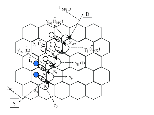
Figure 4: When the device is exposed to air $\rm a_{cc}$ changes. $\rm\Delta a_{A_{1}B_{1}}(\bar{t}_{2})$ and $\rm\Delta a_{B_{1}A_{2}}(\bar{t}_{2})$ become zero, leading to ${\gamma_{11}(\bar{t_{2}})}$=${\gamma_{12}(\bar{t_{2}})}$=$\gamma_{0}$, and $\rm\Delta a_{A_{2}B_{2}}(\bar{t}_{2})$ increases, resulting in ${\gamma_{22}^{\prime}(\bar{t_{2}})}$, which is different from ${\gamma_{22}(\bar{t_{2}})}$ (figure 2(b)). The solid circles represent the air molecules.

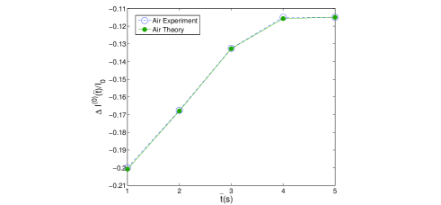
Figure 5: The sensor response $\Delta I^{(0)}(\bar{t})/{I_{0}}$ versus time $\bar{t}$(s) for air. This plot again shows agreement between theory and experiment.

On the other hand, table 2 gives the values of the parameters $\rm\Delta a_{cc}(\bar{t})$ and $\varepsilon_{f}(\bar{t})$ when the DNA-SWNT sensor is exposed to air. When the gas molecules are replaced by air molecules the charge transfer takes place from SWNT to the Air-DNA-base complex, causing an increase in $\rm a_{cc}(\bar{t})$ (positive value) from its modified value due to gas and a decrease in $\varepsilon_{f}(\bar{t})$. The zero value of $\rm\Delta a_{cc}(\bar{t})$ indicates that $\rm a_{cc}$ increases and acquires its pristine value (figure 4). This results in lowering the hopping integral $(\gamma_{ij}=\gamma_{0}\rm exp(-\Delta a_{cc}(\bar{t})/{a_{0}}))$ and hence the transmission function, leading to a decrease in the electron current and therefore an increase in the hole current. A decrease in $\varepsilon_{f}(\bar{t})$ shows that the Fermi level moves towards the valence band. Figure 4 shows the changes in $\rm a_{cc}(\bar{t})$ when air molecules replace the gas molecules. Figure 5 gives the sensor response to air, where the charge transfer from SWNT to the Air-thymine-base complex is larger than the charge transfer from SWNT to the Air-cytosine-base complex. This indicates the sensitivity of the sensor response to the DNA bases. Figures 3 and 5 show a good match between the experimental and theoretical results. Hence, the formula reproduces the current characteristics of the experiment [12].

Using $I(\bar{t})$ the net charge transfer per second can be calculated as $\Delta Q(\bar{t}_{i})=I({\bar{t}_{i}})-I(\bar{t}_{i-1})$. Using the expressions for $G^{(0)}$ and $G^{(1)}$, we find that $I^{(1)}(\bar{t})$ changes with $\gamma_{ij}(\bar{t})$, $\varepsilon_{X_{i}}(\bar{t})$, $\Sigma_{\rm S,\rm D}(\bar{t})$, $\overline{\Delta}(\bar{t})$ and $\frac{\partial\gamma_{ij}(\bar{t})}{\partial\bar{t}}$, $\frac{\partial\varepsilon_{X_{i}}(\bar{t})}{\partial\bar{t}}$, $\frac{\partial\Sigma_{\rm S,\rm D}(\bar{t})}{\partial\bar{t}}$ while $I^{(0)}(\bar{t})$ changes with $\gamma_{ij}(\bar{t})$, $\varepsilon_{X_{i}}(\bar{t})$ and $\Sigma_{\rm S,\rm D}(\bar{t})$. These are some predictions of the model for the experiment. The results for the time-dependent current can be used to calculate the two-time current correlation function and compared with the plots calculated from the experiment [12], figure 1 and will be reported elsewhere.

5 Conclusions

In conclusion, the two-time current correlation function for the experimental data [12] has been calculated and for this system analytical calculations of quantum electronic transport have been presented by setting up a tight-binding model and applying the time-dependent NEGF formalism. The Green’s functions and coupling functions have been expanded using the adiabatic expansion in the slow variable and the Fourier transform has been taken with respect to the fast variable. With the help of the Green’s functions and coupling functions, the zeroth and first order contributions to the current have been investigated. We explicitly calculate the sensor response by considering a form for the hopping integral in terms of $\rm\Delta a_{cc}(\bar{t})$. The sensor response is found to be sensitive to the DNA bases.

Equations (1), (4)-(6) carry the principal results of this paper. The correlation function equation (1) is a measure of the sensitivity and selectivity of the DNA-decorated SWNT sensors and suggest that these gas flow sensors may also be used as DNA sequence detectors, where the pattern of correlation functions may be used as a benchmark for the particular chemical signal encoded in a DNA sequence. Equation (4) presents the zeroth order time-dependent current, which is the Landauer formula that depends on the slow time variable $\bar{t}$. The dependence of the transmission function and hence the current, on $\gamma_{ij}(\bar{t})$ and $\varepsilon_{X_{i}}(\bar{t})$, has been shown by an explicit formula, equation (5). Equation (6) shows the first order contribution to the current for the experiment [12], which is proportional to the zeroth and first order Green’s functions. The formula for the time-dependent current is then used to compare the theoretical results with the experiment. An expression for the net charge transfer per second is obtained using the current.

The numerical and analytical approaches used in this work can be applied to a broad range of systems where gas flows over nano-structures doped with different chemical and biological molecules. This will provide a method for the study of time-dependent electronic transport in low dimensional disordered systems with gas flow. We believe that the analyses done in this manuscript are also applicable to DNA-decorated graphene sensors [36] and give predictions to strengthen future experiments.

References

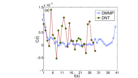
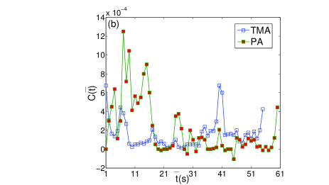
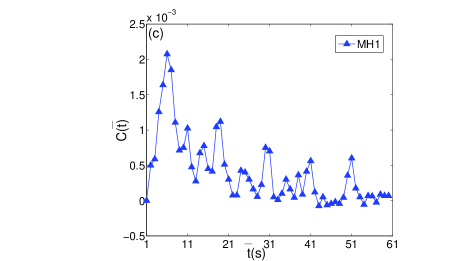
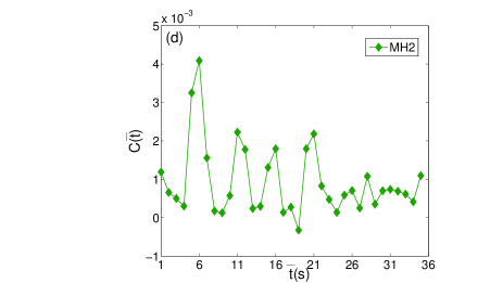
Figure 1: The two-time current correlation function $C(\bar{t})$ versus $\bar{t}$(s) for (a) DMMP + sequence 2 and DNT + sequence 1 (b) TMA + sequence 2 and PA + sequence 1 (c) methanol + sequence 1 and (d) methanol + sequence 2.

Table 1: Values for different parameters used in the calculation of the current with $\gamma_{0}$=2.5eV for methanol with DNA sequence 2. The units of $\varepsilon_{f}$ and $\rm\Delta a_{cc}$ are eV and Å respectively.

• $\hbox{\phantom{\footnotesize\rm 0}}\hbox{\phantom{\footnotesize\rm 0}}\hbox{\phantom{\footnotesize\rm 0}}\bar{t}(s)$	-$\bar{t_{1}}$	-$\bar{t_{2}}$	-$\bar{t_{3}}$	-$\bar{t_{4}}$	-$\hbox{\phantom{\footnotesize\rm 0}}\bar{t_{5}}$
  00$\Delta I^{(0)}(\bar{t})/{I_{0}}$	$0.0151$	$-0.0727$	$-0.08197$	$-0.0728$	$-0.1119$
  00$\varepsilon_{f}(\bar{t})$	-1.68	-3.29	-3.35	-1.83	-2.96
  00$\rm\Delta a_{A_{1}B_{1}}(\bar{t})$	$-0.004$	$-0.004$	$-0.004$	$-0.004$	$-0.004$
  00$\rm\Delta a_{B_{1}A_{2}}(\bar{t})$	$-0.006$	$-0.012$	$-0.012$	$-0.012$	$-0.012$
  00$\rm\Delta a_{A_{2}B_{2}}(\bar{t})$	-—	$-0.006$	$-0.012$	$-0.012$	$-0.012$
  00$\rm\Delta a_{B_{2}A_{3}}(\bar{t})$	-—	-—	$-0.004$	$-0.008$	$-0.008$
  00$\rm\Delta a_{A_{3}B_{3}}(\bar{t})$	-—	-—	-—	$-0.006$	$-0.012$
  00$\rm\Delta a_{B_{3}A_{4}}(\bar{t})$	-—	-—	-—	-—	$-0.006$

Figure 3: The sensor response $\Delta I^{(0)}(\bar{t})/{I_{0}}$ versus time $\bar{t}$(s) for methanol with DNA sequence 2. This plot shows agreement between the theory and experiment. We have found similar results for methanol with the other DNA sequence 1. Experimental data is used from [12] with permission from American Chemical Society.

Table 2: Values for different parameters used in the calculation of the current with $\gamma_{0}$=2.5eV for air.

• $\hbox{\phantom{\footnotesize\rm 0}}\hbox{\phantom{\footnotesize\rm 0}}\hbox{\phantom{\footnotesize\rm 0}}\bar{t}(s)$	-$\bar{t_{1}}$	-$\bar{t_{2}}$	-$\bar{t_{3}}$	-$\bar{t_{4}}$	-$\hbox{\phantom{\footnotesize\rm 0}}\bar{t_{5}}$
  00$\Delta I^{(0)}(\bar{t})/{I_{0}}$	$-0.2008$	$-0.1679$	$-0.1327$	$-0.1157$	$-0.1150$
  00$\varepsilon_{f}(\bar{t})$	-3.55	-3.34	-3.22	-1.48	-2.19
  00$\rm\Delta a_{A_{1}B_{1}}(\bar{t})$	-0	-0	-0	-0	-0
  00$\rm\Delta a_{B_{1}A_{2}}(\bar{t})$	-0.020	-0	-0	-0	-0
  00$\rm\Delta a_{A_{2}B_{2}}(\bar{t})$	--0.012	-0.020	-0	-0	-0
  00$\rm\Delta a_{B_{2}A_{3}}(\bar{t})$	--0.008	--0.008	-0.014	-0	-0
  00$\rm\Delta a_{A_{3}B_{3}}(\bar{t})$	--0.012	--0.012	--0.012	-0.020	-0
  00$\rm\Delta a_{B_{3}A_{4}}(\bar{t})$	--0.006	--0.006	--0.006	--0.006	-0.014

References

- [1] Saito R, Dresselhaus G and Dresselhaus M S 1998 Physical Properties of Carbon Nanotubes (London: Imperical College Press)
- [2] Kong J, Franklin N R, Zhou C, Chapline M G, Peng S, Cho K and Dai H 2000 Science 287 622
- [3] Collins P G, Bradley K, Ishigami M and Zettl A 2000 Science 287 1801
- [4] Li J, Lu Y, Ye Q, Cinke M, Han J and Meyyappan M 2003 Nano Lett. 3 929
- [5] Snow E, Perkins F K 2005 Nano Lett. 5 2414
- [6] Latil S , Roche S and Charlier J C 2005 Nano Lett. 5 2216
- [7] Snow E S, Perkins F K, Houser E J, Badescu S C and Reinecke T L 2005 Science 307 1942
- [8] Shim M, Javey A, Kam N W S and Dai H 2001 J. Am. Chem. Soc. 123 11512
- [9] Qi P, Vermesh O, Grecu M, Javey A, Wang Q, Dai H, Peng S and Cho K J 2003 Nano Lett. 3 347
- [10] Peng S and Cho K 2003 Nano Lett. 3 513
- [11] Latil S, Roche S, Mayou D and Charlier J C 2004 Phys. Rev. Lett. 92 256805
- [12] Staii C, Johnson Jr A T, Chen M and Gelperin A 2005 Nano Lett. 5 1774
- [13] Zheng M, Jagota A, Semke E D, Diner B A, Mclean R S, Lustig S R, Richardson R E and Tassi N G 2003 Nat. Mater. 2 338
- [14] Zheng M et al 2003 Science 302 1545
- [15] Jeng E S, Moll A E, Roy A C, Gastala J B and Strano M S, 2006 Nano Lett. 6 371
- [16] Tu X, Manohar S, Jagota A and Zheng M 2009 Nature 460 250
- [17] Enyashin A N, Gemming S and Seifert G 2007 Nanotechnology 18 245702
- [18] Meng S, Maragakis P, Papaloukas C and Kaxiras E 2007 Nano Lett. 7 45
- [19] Gowtham S, Scheicher R H, Pandey R, Karna S P and Ahuja R 2008 Nanotechnology 19 125701
- [20] Johnson R R, Johnson A T C and Klein M L 2010 Small 6 31
- [21] Gao H and Kong Y 2004 Annu. Rev. Mater. Res. 34 123
- [22] Haug H J W and Jauho A P 2008 Quantum Kinetics in Transport and Optics of Semiconductors (Berlin Heidelberg New York: Springer)
- [23] Nardelli M B 1999 Phys. Rev.B 60 7828
- [24] Meir Y and Wingreen N S 1992 Phys. Rev. Lett. 68 2512
- [25] Wingreen N S, Jauho A P and Meir Y 1993 Phys. Rev.B 48 8487
- [26] Kienle D and Leonard F 2009 Phys. Rev. Lett. 103 026601
- [27] Poonam P and Deo N 2008 Sens. Actuators B Chem. 135 327
- [28] Imry Y 1997 Introduction to Mesoscopic Physics (Oxford: Oxford University Press)
- [29] Lee P A 1986 Physica 140A 169 Lee P A and Ramakrishnan T V 1985 Rev. Mod. Phys. 57 287 Lee P A and Stone A D 1985 Phys. Rev. Lett. 55 1622 Al’tshuler B L, Lee P A and Webb R A Mesoscopic Phenomena in Solids 1991 (New York: North-Holland)
- [30] Datta S 2007 Quantum Transport: Atom to Transistors (Cambridge: Cambridge University Press)
- [31] Hernandez A R, Pinheiro F A, Lewenkopf C H and Mucciolo E R 2009 Phys. Rev.B 80 115311
- [32] Datta S 1995 Electronic Transport in Mesoscopic Systems (Cambridge: Cambridge University Press)
- [33] Chen Y R, Zhang L and Hybertsen M S 2007 Phys. Rev.B 76 115408
- [34] Falko V 2006 Quantum transport of chiral electrons in graphene I (Lecture note in ‘College on Physics of Nano-Devices’) The Abdus Salam International Centre for Theoretical Physics (Trieste: Italy)
- [35] Ghosh S, Gadagkar V and Sood A K 2005 Chem. Phys. Lett. 406 10
- [36] Lu Y, Goldsmith B R, Kybert N J and Johnson A T C 2010 Appl. Phys. Lett. 97 083107
-
1.68 3.29 3.35 1.83 2.96 — — — — — — — — — —
-
3.55 3.34 3.22 1.48 2.19 0 0 0 0 0 0.020 0 0 0 0 -0.012 0.020 0 0 0 -0.008 -0.008 0.014 0 0 -0.012 -0.012 -0.012 0.020 0 -0.006 -0.006 -0.006 -0.006 0.014