Quantum Phase Diagram and Excitations for the One-Dimensional $S=1$ Heisenberg Antiferromagnet with Single-Ion Anisotropy

Abstract

We investigate the zero-temperature phase diagram of the one-dimensional $S=1$ Heisenberg antiferromagnet with single-ion anisotropy. By employing high-order series expansions and quantum Monte Carlo simulations we obtain accurate estimates for the critical points separating different phases in the quantum phase diagram. Additionally, excitation spectra and gaps are obtained.

I Introduction

Interest in one-dimensional $S=1$ antiferromagnets is long-standing and can be traced back to the original work by Haldane.Haldane (1983a, b) By analyzing the presence of topological terms in effective field-theories for one-dimensional antiferromagnets he conjectured that integer-spin chains display a ground-state with exponentially decaying spin-spin correlations and a gapped excitation spectrum, properties markedly different from those displayed by the exactly solvable $S=1/2$ chain. Despite early controversy, this so called “Haldane conjecture” is now supported by solid numericalWhite and Huse (1993) and experimentalRegnault et al. (1994); Kenzelmann et al. (2002) evidence (for a review of earlier results, see Ref. Affleck, 1989).

We are interested in the anisotropic $S=1$ antiferromagnetic chain described by the Hamiltonian

$${\mathcal{H}}=J\sum_{i}\vec{S}_{i}\cdot\vec{S}_{i+1}-D\sum_{i}({S}^{z}_{i})^{2}~{}.$$ (1)

The single-ion anisotropy term proportional to $D$ is relevant in accounting for the magnetic properties of a number of compounds: ${\rm CsNiCl_{3}}$ (weak axial anisotropy, Refs. Steiner et al., 1987 and Kenzelmann et al., 2002), NENP [${\rm Ni(C_{2}H_{8}N_{2})_{2}NO_{2}(ClO_{4})}$] (weak axial anisotropy, Ref. Renard et al., 1988), ${\rm CsFeBr_{3}}$, NENC [${\rm Ni(C_{2}H_{8}N_{2})_{2}Ni(CN)_{4}}$] and DTN [${\rm NiCl_{2}-4SC(NH_{2})_{2}}$] (strong planar anisotropy, Refs. Dorner et al., 1988, Orendác̆ et al., 1995 and Zapf et al., 2006 respectively); DTN is particularly interesting due to Bose-Einstein condensation of spin excitations under a magnetic field.Zapf et al. (2006); Giamarchi et al. (2008) The model defined by Eq. (1) is also very appealing from a purely theoretical perspective: the single-ion anisotropy $D/J$ controls the magnitude of quantum fluctuations and stabilizes different phases that, along with the quantum critical points separating them, have been extensively investigated. Botet et al. (1983); Glaus and Schneider (1984); Schulz (1986); Papanicolaou and Spathis (1990); Sakai and Takahashi (1990); Golinelli et al. (1992); Chen et al. (1993, 2003); Boschi et al. (2003); Boschi and Ortolani (2004); Campos Venuti et al. (2006); Tzeng and Yang (2008); Tzeng et al. (2008)

For large positive values of the single-ion anisotropy $D/J$ the system is in an Ising-like Néel phase characterized by finite staggered magnetization at zero temperature $T=0$ and displaying a gap for holon-like excitations, that we will discuss later in Sec. III.2. Comparatively less well understood is the so-called large-$D$ phase for large negative values of $D/J$, first investigated in detail by Papanicolaou and Spathis.Papanicolaou and Spathis (1990) The ground-state in the large-$D$ phase smoothly evolves from the ground-state for $D/J\rightarrow-\infty$, simply given by the tensor-product of $S_{i}^{z}=0$ states at each site. The lowest-energy excitations in this phase reside in the $S_{T}^{z}=\pm 1$ sector and were termed excitons and anti-excitons in Ref. Papanicolaou and Spathis, 1990, where the existence of bound-states was also verified.

Physical intuition was gained about the intermediate phase observed for small values of $|D|/J$, including the isotropic point $D/J=0$ analyzed by Haldane,Haldane (1983a, b) by studying an extended $S=1$ model with biquadratic interactions

$${\mathcal{H}}_{\rm AKLT}=J\sum_{i}\left[\vec{S}_{i}\cdot\vec{S}_{i+1}+\beta(\vec{S}_{i}\cdot\vec{S}_{i+1})^{2}\right]~{}.$$ (2)

Affleck, Kennedy, Lieb and Tasaki (AKLT)Affleck et al. (1987) showed that this Hamiltonian is exactly solvable at $\beta=1/3$, where it displays a simple valence-bond solid (VBS) ground-state with gapped excitations. den Nijs and Rommelseden Nijs and Rommelse (1989) later suggested that this VBS state can be interpreted as a “fluid” with positional disorder and long-range antiferromagnetic order, characterized by a finite expectation value for the string-operator,

$${\mathcal{O}}_{s}(r)={S}^{z}_{0}\exp\left(i\pi\sum_{k=1}^{r-1}{S}^{z}_{k}\right){S}^{z}_{r}~{},$$ (3)

in the limit $r\rightarrow\infty$, associated with the breaking of a hidden $\mathbb{Z}_{2}\times\mathbb{Z}_{2}$ symmetry.Kennedy and Tasaki (1992) Since the ground-state at $\beta=0$ has been shownWhite and Huse (1993) to exhibit long-ranged string correlations and is adiabatically connected to the ground-state at $\beta=1/3$ (see e.g. Ref. Schollwöck et al., 1996), one concludes that the Haldane phase has a VBS character. We remark that interest in Haldane-like phases exhibiting long-range string correlations has been renewed and proposals for investigating string-order in cold atomic systems have recently been made.García-Ripoll et al. (2004); Dalla Torre et al. (2006)

In this paper, we are primarily interested in improving on previous estimates for the location of the large-$D$—Haldane (DH) and the Haldane—Néel (HN) critical points. Improved results may be used as benchmarks for further tests on the applicability of quantum information tools to detect quantum phase transitions in the model Eq. (1).Tzeng and Yang (2008); Tzeng et al. (2008) Additionally, we obtain results for the excitation spectra and gaps in the large-$D$ and Néel phases that may be of experimental relevance. We also show that a series expansion method previously applied for calculating the Haldane gapSingh (1996) yields an incorrect result, and we propose a different approach for future work.

II Methods

We have investigated the $S=1$ antiferromagnetic chain described by the Hamiltonian Eq. (1) by combining high-order series expansions and quantum Monte Carlo (QMC) simulations. Technical details are described in this Section.

II.1 Series Expansions

Numerical linked-cluster expansions have been extensively employed in the investigation of quantum magnets (for detailed accounts the reader is referred to Refs. Gelfand and Singh, 2000 and Oitmaa et al., 2006; a closely related method is discussed in Refs. Knetter and Uhrig, 2000 and Knetter et al., 2003) and have been recently derived by some of usOitmaa and Hamer (2008) for the square lattice version of the Hamiltonian Eq. (1). Among the method’s many appealing features we highlight its applicability to the study of excitations and dynamical responses, a notoriously difficult task within alternative numerical approaches, following the procedure originally devised by Gelfand.Gelfand (1996)

Basically, the linked-cluster method relies on a suitable decomposition of the lattice Hamiltonian under investigation,

$${\mathcal{H}}={\mathcal{H}}_{\rm 0}+\lambda{\mathcal{V}}~{}.$$ (4)

It is assumed that the ground-state of the unperturbed Hamiltonian ${\mathcal{H}}_{\rm 0}$ is known and can be written as a tensor product of local states. One proceeds by deriving a standard Rayleigh-Schrödinger perturbative expansion for connected clusters comprised of an increasingly large number of sites and, at each step, one subtracts contributions from embedded subclusters containing fewer sites. In this way, long series for ground-state quantities and excited states can be exactly calculated up to a certain order in the expansion parameter $\lambda$, that are then analyzed by means of any suitable extrapolation technique (in this paper we adopt a standard Padé analysis). In what follows, we present the different expansions employed in the present study.

II.1.1 Large-$D$ Expansion

For investigating the phase stabilized for large negative values of $D/J$ we consider the single-ion term as our unperturbed Hamiltonian

$${\mathcal{H}}^{\rm LDE}_{\rm 0}=-D\sum_{i}({S}^{z}_{i})^{2}~{},$$ (5)

the superexchange terms in Eq. (1) being treated as the perturbation ${\mathcal{V}}^{\rm LDE}$

$${\mathcal{V}}^{\rm LDE}=J\sum_{i}\left[S^{z}_{i}S^{z}_{i+1}+\frac{1}{2}\left(S^{+}_{i}S^{-}_{i+1}+S^{-}_{i}S^{+}_{i+1}\right)\right]~{}.$$ (6)

The (non-degenerate) ground-state of ${\mathcal{H}}^{\rm LDE}_{\rm 0}$ is simply given by tensor products of $S_{i}^{z}=0$ states for all sites $i$ on the chain and, in what follows, we refer to this expansion as the large-$D$ expansion (LDE). Results for the ground-state energy density obtained from an LDE series comprising terms of up to $\lambda^{30}$ are shown in Fig. 1 (open diamonds). Shorter series have been obtained for the excited states (up to $\lambda^{14}$), the results being presented in Sec. III.1.

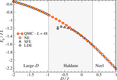
Figure 1: (Color online) Ground-state energy density for the model described by Eq. (1) as a function of the single-ion anisotropy $D/J$. QMC results are shown as filled circles and have been obtained for a lattice with $L=48$ sites. Empty symbols correspond to results from the series expansions: large-$D$ expansion (LDE, diamonds), Néel expansion (NE, squares) and staggered-field expansion (SFE, triangles). The vertical dashed lines highlight our best estimates for the location of the critical points: $D_{\rm C}^{\rm DH}/J=-0.971(5)$ for the point separating the large-$D$ and Haldane phases, and $D_{\rm C}^{\rm HN}/J=0.316(2)$ for the HN phase transition (see main text). Unless visible, error bars are smaller than depicted symbols.

II.1.2 Néel Expansion

A suitable linked-cluster expansion for large positive values of $D/J$ is obtained by choosing the unperturbed Hamiltonian

$${\mathcal{H}}^{\rm NE}_{\rm 0}=J\sum_{i}S^{z}_{i}S^{z}_{i+1}-D\sum_{i}({S}^{z}_{i})^{2}~{},$$ (7)

and starting from a perfectly ordered Néel unperturbed ground-state. The remaining fluctuation terms in Eq. (1) are our perturbation ${\mathcal{V}}^{\rm NE}$

$${\mathcal{V}}^{\rm NE}=\frac{J}{2}\sum_{i}\left(S^{+}_{i}S^{-}_{i+1}+S^{-}_{i}S^{+}_{i+1}\right)~{},$$ (8)

and we refer to the resulting expansion as the Néel expansion (NE). The ground-state energy and the staggered magnetization in the Néel phase have been calculated from a NE comprising terms of to $\lambda^{18}$ (results for the ground-state energy are depicted as open squares in Fig. 1). Series for the single-particle excitations have been obtained from expansions up to $\lambda^{14}$; the results are discussed in Sec. III.2.

II.1.3 Staggered-Field Expansion

We have also considered a series expansion originally devised by Singh,Singh (1996) here dubbed as the staggered-field expansion (SFE), obtained by considering a Hamiltonian including an artificial staggered-field term

$$\begin{split}{\mathcal{H}}^{\rm SFE}=J\sum_{i}\left[S^{z}_{i}S^{z}_{i+1}+\frac{\lambda}{2}\left(S^{+}_{i}S^{-}_{i+1}+S^{-}_{i}S^{+}_{i+1}\right)\right]\\ -D\sum_{i}({S}^{z}_{i})^{2}+(1-\lambda)\sum_{i}(-1)^{i}{S}^{z}_{i}~{}.\end{split}$$ (9)

(Terms proportional to $\lambda$ are our perturbation ${\mathcal{V}}^{\rm SFE}$ and the remaining ones define the unperturbed Hamiltonian ${\mathcal{H}}_{0}^{\rm SFE}$.) The unperturbed ground-state is a perfectly ordered Néel state, as in the case of the NE, and the Hamiltonian Eq. (1) is recovered in the limit $\lambda=1$, where the last term in Eq. (9) vanishes. This staggered-field term is included in order to prevent the condensation of solitons before $\lambda=1$, as discussed in Ref. Singh, 1996, allowing one to obtain a seemingly precise estimate for the Haldane gap at $D/J=0$. Results for the ground-state energy per site obtained from an SFE including terms up to $\lambda^{18}$ are represented by open triangles in Fig. 1: it is clear from this plot that the SFE systematically underestimates $E_{\rm 0}/L$ towards the DH critical point and we will address this issue later in Sec. III.3, along with our results for the gap at $D/J=0$.

II.2 Quantum Monte Carlo

QMC simulations have been performed by employing the ALPS (Algorithms and Libraries for Physics Simulations) libraries’ Albuquerque et al. (2007) implementation of the directed loops algorithm Syljuåsen and Sandvik (2002); Alet et al. (2005) in the Stochastic Series Expansion (SSE) framework.Sandvik (1999) We have simulated the model Eq. (1) on lattices with length $L$ ranging from 24 to 48, applying periodic boundary conditions. In order to assess ground-state properties, simulations were performed for temperatures $T=1/100<1/2L$: results for the spin-stiffness $\rho_{\rm S}$ (Fig. 2) and the Binder cummulant $Q_{2}$ [Eq. (11), Fig. 7] are converged, within statistical errors, to their ground-state expectation values for this value of $T$, as verified by running preliminary QMC simulations for various temperatures. Results for the ground-state energy density $E_{\rm 0}/L$ for a lattice $L=48$ are shown in Fig. 1: the data for $E_{\rm 0}/L$ are essentially converged for this system size (within statistical errors, as we can conclude by comparing against results obtained from smaller lattice sizes, not shown here), and good agreement is obtained with the results from the LDE and NE described in the previous subsection.

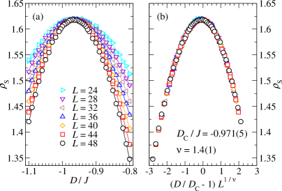
Figure 2: (Color online) (a) Spin-stiffness $\rho_{\rm S}$ as a function of the single-ion anisotropy close to the critical point separating the large-$D$ and Haldane phases (lines are only guides to the eye). Results have been obtained from QMC simulations for values of $L$ ranging from $24$ to $48$ and error bars are smaller than depicted symbols. (b) Data collapse is achieved for $D_{\rm C}^{\rm DH}/J=-0.971(5)$ and $\nu=1.4(1)$ (see main text).

III Numerical Results

We present estimates for the location of the quantum critical points in the phase diagram of the Hamiltonian Eq. (1) and results for the excitation spectra and gaps obtained by using the numerical procedures described in the previous section.

III.1 Large-$D$ — Haldane Phase Transition

The Gaussian quantum phase transition between the large-$D$ and the Haldane phases has been studied in a number of recent works.Chen et al. (2003); Boschi et al. (2003); Tzeng and Yang (2008); Tzeng et al. (2008) The critical point was pinpointed by Chen et al.Chen et al. (2003)  by performing exact diagonalizations of small clusters with twisted boundary conditions. Furthermore, these authors verified that the DH transition is described by a conformal field-theory with central charge $c=1$, as further confirmed by Boschi et al. Boschi et al. (2003) using a combined field-theoretic and numerical analysis. More recently, Tzeng and collaborators,Tzeng and Yang (2008); Tzeng et al. (2008) motivated by the current interest in applying concepts and tools from quantum information theory to the study of condensed matter systems,Amico et al. (2008) showed that the DH phase transition can be located by investigating the scaling behavior of the ground-state fidelity and the entanglement entropy, and arrived at the estimateerr $D_{\rm C}^{\rm DH}/J=0.97$. Here, we investigate the DH transition employing the numerical methods described in Sec. II.

III.1.1 Spin Stiffness

In Fig. 2(a) we show our QMC results for the spin-stiffness $\rho_{\rm S}$, obtained in terms of the winding number $w$, $\rho_{\rm S}=3\langle w^{2}\rangle/2\beta$ ($\beta$ is the inverse temperature),Sandvik (1997) for system sizes $L$ ranging from 24 to 48. Away from the critical point, both the large-$D$ and the Haldane phases display exponentially decaying spin correlations and therefore we expect $\rho_{\rm S}$ to approach zero in the thermodynamic limit, a trend clearly discernible in Fig. 2(a). On the other hand, close to the critical point, where the correlation length $\xi$ diverges, the spin-stiffness is expectedSachdev (1999) to scale as $\rho_{\rm S}\sim L^{2-z-d}$. Since $d=1$ is the spatial dimension and the dynamic critical exponent is expected to be $z=1$ (see below), one expects $\rho_{\rm S}$ to assume a size independent value at the transition point (similarly to what happens for the $S=1/2$ chain with easy-plane anisotropy, see Ref. Laflorencie et al., 2001), as confirmed by our QMC data plotted in Fig. 2(a). We remark that this “peaked behavior” for $\rho_{\rm S}$ is a signature of a transition between two phases with exponentially decaying spin correlations and it should be contrasted with the “crossing behavior” for $\rho_{\rm S}L$ observed in more conventional order-disorder quantum transitions in two-dimensional systems (see e.g. Refs. Wang et al., 2006; Wenzel et al., 2008; Albuquerque et al., 2008).

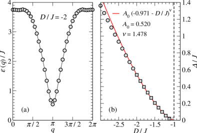
Figure 3: (Color online) (a) Excitation spectrum in the large-$D$ phase, for $D/J=-2$, obtained from the LDE. (b) Gap for excitations ($q=\pi$) in the large-$D$ phase as a function of $D/J$, again obtained from the LDE (the series become badly behaved beyond the rightmost data point). The continuous line has been obtained by fitting the scaling function $\Delta/J=A_{\rm 0}[(D_{\rm C}^{\rm DH}-D)/J)]^{z\nu}$, assuming $z=1$, to the data points depicted as squares, using the QMC estimate $D_{\rm C}^{\rm DH}/J=-0.971$ (vertical dashed line). In both panels, with the exception of the rightmost data point in (b), error bars are smaller than the depicted symbols.

In order to estimate the location of the quantum critical point $D_{\rm C}^{\rm DH}/J$ and the correlation length critical exponent $\nu$, we assume the scaling ansatz

$$\rho_{\rm S}(t,L)=f_{\rho_{\rm S}}(tL^{1/\nu})~{},$$ (10)

with reduced coupling $t=(D/D_{\rm C}^{\rm DH}-1)$. Data collapse is achieved for $D_{\rm C}^{\rm DH}/J=-0.971(5)$ and $\nu=1.4(1)$ [Fig. 2(b)], values in good agreement with the ones from Ref. Tzeng and Yang, 2008 ($D_{\rm C}^{\rm DH}/J=-0.97$ and $\nu=1.42$, $1.45$).err We use our result $\nu=1.4(1)$ to calculate the Luttinger-liquid parameter $K$ by employing the relationBoschi et al. (2003); Tzeng and Yang (2008); Tzeng et al. (2008) $\nu=1/(2-K)$ and obtain $K=1.29(5)$, consistent with previous findings.Boschi et al. (2003); Tzeng and Yang (2008); Tzeng et al. (2008) Additionally, the bulk spin-stiffness at the critical point is estimated to be $\rho_{\rm S}^{\rm DH}=1.619(5)$.

III.1.2 Excitations

The lowest-lying excitations in the large-$D$ phase lie in the $S^{z}_{\rm T}=\pm 1$ sectors and we calculate their dispersion relation by applying the LDE presented in Sec. II.1.1. Results obtained after a standard Padé analysis are shown in Fig. 3(a) for $D/J=-2$. As we approach the DH transition from the large negative $D/J$ side, the gap at $q=\pi$ drops to zero, and the dispersion in that neighbourhood becomes linear, a trend already noticeable for $D/J=-2$ [Fig. 3(a)] and consistent with a dynamic critical exponent $z=1$. We remark that this behavior is not reproduced in the strong-coupling analysis by Papanicolaou and Spathis,Papanicolaou and Spathis (1990) which gives a quadratic dispersion relation (this is also the case in our results for couplings deep into the large-$D$ phase, not shown here). The dependence of the gap at $q=\pi$ on $D/J$ is shown in Fig. 3(b). Unfortunately, the series convergence becomes irregular beyond the rightmost data point in the figure, preventing us from obtaining independent estimates for $D_{\rm C}^{\rm DH}/J$ and for the critical exponents. In order to partially circumvent this problem, we fit the scaling function $\Delta/J=A_{\rm 0}[(D_{\rm C}^{\rm DH}-D)/J)]^{z\nu}$, assuming $z=1$, to the data points depicted as squares in Fig. 3(b). By fixing $D_{\rm C}^{\rm DH}/J=-0.971$, as estimated from our QMC data, the data is fitted for $\nu=1.478$, a value consistent with the QMC result $\nu=1.4(1)$ and that further confirms that indeed $z=1$.

III.2 Haldane — Néel Phase Transition

The Néel phase for large positive values of $D/J$ has a twofold degenerate ground-state and therefore the HN quantum phase transition is expected to belong to the universality class of the two-dimensional Ising model. Chen et al.Chen et al. (2003) located the HN critical point by applying a phenomenological renormalization group analysis to data from exact diagonalization of clusters with up to 16 sites. More recently the estimateerr $D_{\rm C}^{\rm HN}/J=0.31$ was obtained by Tzeng and Yang,Tzeng and Yang (2008) who studied the scaling behavior of the ground-state fidelity close to the HN critical regime.

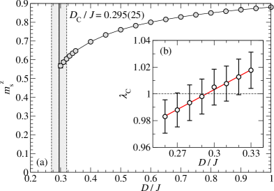
Figure 4: (Color online) (a) Staggered magnetization per site $m^{z}_{\rm s}$ as a function of $D/J$ in the Néel phase, obtained from the NE by applying a Padé analysis. (b) Location of the poles $\lambda_{\rm C}$ in the Dlog Padé approximants for the staggered magnetization series, as a function of $D/J$. In both panels, lines are only guides to the eye.

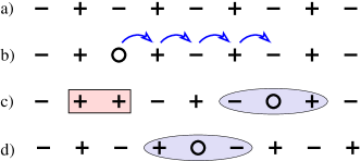
Figure 5: (Color online) Pseudo-particle representation of the $S=1$ chain.den Nijs and Rommelse (1989) Sites with $S^{z}_{i}=\pm 1$ are seen as being occupied by spin-half particles with pseudo-spin components $\tilde{S}^{z}_{i}=\pm 1/2$ (depicted as $+$’s and $-$’s) and sites with $S^{z}_{i}=0$ as being empty (occupied by “holes”, represented by circles) In this language, the Néel ground-state corresponds to an undoped antiferromagnet (a). Excited states are obtained by doping the system with holes (b). As depicted in (c), a hole doped into the system decays into “spinon” (enclosed by the rectangle) and holon (enclosed by the ellipsis) constituents [the state depicted in (c) is obtained from the state in (b) by allowing the hole to “hop” four sites to the left, as indicated by the arrows]. Since a spinon costs an energy $\sim J$, excited states containing only a holon (d) are expected to have lower energy (see main text).

III.2.1 Staggered Magnetization

We first employ the NE discussed in Sec. II.1.2 in order to calculate the staggered magnetization, $m^{z}_{\rm s}=\langle(-1)^{i}S^{z}_{i}\rangle/L$, as a function of $D/J$. The results obtained by applying standard Padé approximant extrapolations to the series in $\lambda$ are shown in Fig. 4(a). The position of the HN quantum critical point can be determined by a Dlog Padé analysis of $m^{z}_{\rm s}$ as a function of $\lambda$: as shown in Fig. 4(b), the estimate $D_{\rm C}^{\rm HN}/J=0.295(25)$ [highlighted as the shaded region in Fig. 4(a)] for the HN critical point is simply obtained as the range of values for $D/J$ consistent with a pole at $\lambda=1$, where the full Hamiltonian Eq. (1) is recovered. From the Padé extrapolation we also obtain an estimateexp $\beta=0.147(13)$ for the critical exponent associated to $m^{z}_{\rm s}$, which is somewhat larger than, but not incompatible with, the exact result $\beta=1/8$ for the 2D Ising universality class. We also note that there is little sign of $m^{z}_{\rm s}$ vanishing in the shaded region in Fig. 4(a): this can be explained by the small value of the expected critical exponent $\beta=1/8$, which implies that $m^{z}_{\rm s}$ plunges steeply to zero at the critical point, a behavior which naive Padé approximants will hardly pick up.

III.2.2 Excitations

More accurate estimates for $D_{\rm C}^{\rm HN}/J$ can be obtained by analyzing excited states above the Néel ground-state. At this point, following den Nijs and Rommelse,den Nijs and Rommelse (1989) it is useful to interpret the $S=1$ chain as a diluted system of $\tilde{S}=1/2$ pseudo-particles: as we show in Fig. 5, sites with $S^{z}_{i}=\pm 1$ are seen as being occupied by spin-half particles with pseudo-spin components $\tilde{S}^{z}_{i}=\pm 1/2$ and sites where $S^{z}_{i}=0$ as being empty (occupied by “holes”). Using this language, the Néel ground-state is equivalent to an “undoped” antiferromagnet [Fig. 5(a)] and, for small (positive) values of $D/J$, the low-lying excited states lie in the “one-hole sector” (containing one site with $S^{z}_{i}=0$). Interestingly enough, the situation is reminiscent of spin-charge separation in one-dimensional fermionic systems (see e.g. Ref. Dagotto, 1994) where a hole doped into the system [as depicted in Fig. 5(b)] fractionalizes into “holon” and “spinon” constituents [respectively enclosed by an ellipsis and a rectangle in Fig. 5(c)].

Since one spinon (two consecutive sites with the same pseudo-spin component) has an energetic cost $\sim J$, we expect $S^{z}_{T}=0$ states solely displaying a holon to have a lower excitation energy, as confirmed by our results below. Such a holon state is depicted in Fig. 5(d): we replace one pseudo-spin in the Néel configuration shown in Fig. 5(a) by a hole and flip all pseudo-spins to its right. Antiferromagnetic correlations “across the hole” allow for the hole to delocalize, lowering the energy of holon excited states.Dagotto (1994) Furthermore, these holon excitations can be seen as precursors of the ground-state in the Haldane phase: as shown by Nijs and Rommelse,den Nijs and Rommelse (1989) VBS states can be interpreted as a fluid with positional disorder and long-range antiferromagnetic order. This picture is consistentden Nijs and Rommelse (1989) with the holon state depicted in Fig. 5(d), but not with the holon-spinon excitation shown in Fig. 5(b-c).vbs Therefore, the HN critical point can be determined by locating the value $D_{\rm C}^{\rm HN}/J$ where the gap for the holon excitations vanishes.

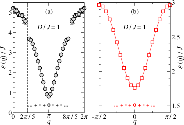
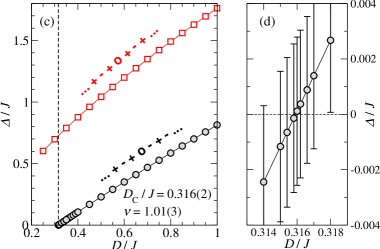
Figure 6: (Color online) (a) Spectrum for “holon” excitations [Fig. 5(d)] at $D/J=1$. The vertical dashed lines indicate momenta for which the NE expansion seemingly diverges. (b) Spectrum for “holon-spinon” excitations [Fig. 5(b-c)], also for $D/J=1$. (c) Excitation gaps as a function of $D/J$. The gap for holon excitations ($q=\pi$, black circles) vanishes linearlyexp [$\nu=1.01(3)$] at $D_{\rm C}^{\rm HN}/J=0.316(2)$ as seen in the magnified plot (d). Data points in all panels were obtained by applying a Padé analysis to the results obtained from the NE.

Results for the spectrum of holon excitations obtained from the NE are shown in Fig. 6(a) for $D/J=1$. We remark that the series seemingly diverges at the commensurate momenta $q=2\pi/5$ and $q=8\pi/5$ [indicated by the vertical dashed lines in Fig. 6(a)] and that the results at higher energies have a rather poor convergence, as indicated by the relatively large error bars in the figure. This suggests that holon excitations decay into multi-holon states and that a continuum of excited states exists at high-energies. Unfortunately, the poor convergence of the (short) series for two- and three-holon excited states, obtained by applying the procedure described in Ref. Zheng et al., 2001, prevents us from further analyzing this issue, which is left open to future investigations. On the other hand, our results for low-energy excitations around $q=\pi$ are nicely converged, allowing us to precisely locate the critical point. In Figs. 6(c-d) we show the dependence of the gap $\Delta/J$ for holon excitations on $D/J$ and we can see it vanishes at $D_{\rm C}^{\rm HN}/J=0.316(2)$, with a critical exponentexp $\nu=1.01(3)$ (directly obtained from the Padé analysis) consistent with the 2D Ising universality class.

For the sake of comparison, we also show the dispersion relation for the $S^{z}_{T}=\pm 1$ holon-spinon [Fig. 5(b-c)] in Fig. 6(b), also for $D/J=1$. The dependence of the gap at $q=0$ on $D/J$ is shown in Fig. 6(c). Note that our results indicate that the energy of this excitation remains finite at the transition, confirming that a holon-spinon state has a higher excitation energy than an isolated holon state. As we see in the plot Fig. 6(c), for large values of $D/J$ the difference in energy between holon-spinon and holon excited states is approximately $J$, confirming our qualitative analysis above.

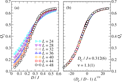
Figure 7: (Color online) (a) Staggered magnetization Binder cumulant $Q_{\rm 2}$ [see Eq. (11)] for couplings $D/J$ close to the Haldane—Néel critical point, as obtained from QMC simulations for system sizes $L$ ranging from 24 to 48. (b) Data collapse is achieved for $D_{\rm C}^{\rm HN}/J=0.312(6)$ and $\nu=1.1(1)$.

III.2.3 Binder Cumulant

The previous findings are confirmed by our QMC results for the second order Binder cumulant $Q_{2}$ for the staggered magnetization $m^{z}_{\rm s}$, given by

$$Q_{2}=1-\frac{\langle(m_{\rm s}^{z})^{4}\rangle}{3\langle(m_{\rm s}^{z})^{2}\rangle^{2}}~{}.$$ (11)

$Q_{2}$ is expected to display universal behavior in the critical regime and results obtained from different lattice sizes should cross close to the critical point, as confirmed by the data shown in Fig. 7(a). In order to estimate the critical point we assume the scaling ansatz $Q_{2}(t,L)=f_{Q_{2}}(tL^{1/\nu})$, with $t=(D/D_{\rm C}^{\rm HN}-1)$. Data collapse is achieved for $D_{\rm C}^{\rm HN}/J=0.312(6)$ and $\nu=1.1(1)$, as shown in Fig. 7(b), consistent with the estimates obtained from the NE. A slightly smaller value, $D_{\rm C}^{\rm HN}/J=0.310(6)$, is estimated from a data collapse obtained by fixing the critical exponent to the known value for the 2D Ising universality class, $\nu=1$.

Additionally, from the data collapse displayed in Fig. 7(b) we arrive at the estimate $Q_{2}^{\ast}=0.515(10)$ for the value assumed by the Binder cummulant at the critical point, markedly different from the known resultKamieniarz and Blöte (1993) $Q_{2}^{\ast}=0.61069...$ for the two-dimensional Ising universality class. This discrepancy can be ascribed to differences in the way $Q_{2}$ is calculated in classical and quantum Monte Carlo simulations: although the $d$-dimensional quantum system is indeed formally equivalent to a classical model in $d+1$ dimensions, equal-time expectation values for diagonal operators are averaged along the imaginary-time direction in quantum simulations. In other words, our results for $Q_{2}^{\ast}$ should be consistent with the ones obtained for the classical two-dimensional Ising model if the moments of the magnetization appearing in the definition Eq. (11) are evaluated along individual lines on the square lattice. Since, to the best of our knowledge, no such calculation has been done, this prevents us from comparing our estimate $Q_{2}^{\ast}=0.515(10)$ with published results. We remark that a similar situation was observed in Ref. Wang et al., 2006 for $S=1/2$ bilayers, expected to belong to the universality class of the classical Heisenberg model in three dimensions.

III.3 Haldane Gap

Finally, we have investigated the SFE introduced by SinghSingh (1996) and discussed in Sec. II.1.3 in order to estimate the Haldane gap at $D/J=0$. Singh assumes that the magnon gap in the Néel phase of the SFE system will extrapolate continuously to the Haldane gap as $\lambda\rightarrow 1$, in spite of the phase transition that must occur at or before $\lambda=1$. The extrapolated value for the magnon gap, $\Delta/J=0.42(1)$,gap obtained from a series involving terms of up to $\lambda^{10}$ as presented in Ref. Singh, 1996, is indeed consistent with the high-precision result for the Haldane gap $\Delta/J=0.41050(2)$ from density-matrix renormalization group (DMRG) calculations.White and Huse (1993) However, higher-order Padé approximants for an extended series comprising terms up to $\lambda^{14}$ show a clear trend towards smaller values and we arrive at the considerably lower value $\Delta/J=0.23(6)$. It is thus obvious that a more careful analysis is required. If we apply a change of variable $\delta=1-\sqrt{1-\lambda}$ to the series, following Huse,Huse (1988) then Padé approximants for the series in $\delta$ show a vanishing magnon gap, $\Delta/J=0.00(1)$, at the transition point $\lambda=1$. The failure to yield correct results for the Haldane gap, combined with the fact that it systematically underestimates the ground-state energy towards the DH critical point, as mentioned in Sec. II.1.3 in connection with Fig. 1, strongly suggests that the SFE approach is not appropriate for estimating results for the integer-spin Haldane systems.

We recall that a Néel state is chosen as the unperturbed state when performing the SFE, and the VBS character of the Haldane phase is ignored. We expect physical results to be obtainable from a different expansion assuming the AKLT model [$\beta=1/3$ in Eq. (2)] as the unperturbed Hamiltonian and starting from the exact VBS ground-stateAffleck et al. (1987) at $\beta=1/3$, treating $\lambda=(\beta-1/3)$ as the expansion parameter. Such an expansion would require the application of the linked-cluster formalism to valence-bond states, something that, to the best of our knowledge, has not yet been tried and that would constitute an interesting topic for future work.

IV Conclusions

Summarizing, we have investigated the one-dimensional $S=1$ antiferromagnet with single-ion anisotropy, described by the Hamiltonian Eq. (1), by means of linked-cluster series expansions and QMC simulations. Our estimates for the zero-temperature phase transitions in this model are more precise than previous ones and could be used as benchmarks in future explorations of the applicability of quantum information tools to the study of quantum critical phenomena.

Our best estimate for the DH critical point [$D_{\rm C}^{\rm DH}/J=0.971(5)$] has been obtained from a scaling analysis of the spin-stiffness $\rho_{\rm S}$ from QMC simulations. The spin-stiffness remains finite at the transition in the thermodynamic limit [$\rho_{\rm S}^{\rm DH}=1.619(5)$] and vanishes elsewhere, implying a “peaked behavior” for finite systems. Our result for $D_{\rm C}^{\rm DH}$ agrees with the estimateerr obtained by Tzeng et al.Tzeng and Yang (2008) [$D_{\rm C}^{\rm DH}=0.97$], the same being true for the estimate for the correlation length critical exponent: $\nu=1.4(1)$ (present work) and $\nu=1.42$, $1.45$ (Ref. Tzeng and Yang, 2008). We have further obtained results for the dispersion relation and gap for excitations in the large-$D$ region that may be of direct experimental relevance given, for instance, the current interest on the large-$D$ compound DTN.Zapf et al. (2006); Giamarchi et al. (2008) Our series for the excited states in the large-$D$ phase have a considerably more extended range of applicability compared to the strong coupling results of Papanicolaou and Spathis,Papanicolaou and Spathis (1990) and are available on request.

Precise results for the HN phase transition have been obtained from a linked-cluster expansion (NE) for holon-like excitations. By analyzing the gap for these excited states we have arrived at the estimates $D_{\rm C}^{\rm HN}/J=0.316(2)$ and $\nu=1.01(3)$. The former compares well with the resulterr $D_{\rm C}^{\rm HN}/J=0.31$ from Ref. Tzeng and Yang, 2008 while the latter confirms that the HN transition belongs to the universality class of the two-dimensional Ising model, with the exact exponent $\nu=1$.

Finally, we have shown evidence that the SFE expansion of SinghSingh (1996) does not converge to the Haldane gap at $D/J=0$. Instead, we propose an expansion around the AKLT state [the exact ground-state for the Hamiltonian Eq. (2) with $\beta=1/3$],Affleck et al. (1987) which we hope to explore in future work.