Algorithmic complexity and randomness in elastic solids

Abstract

A system comprised of an elastic solid and its response to an external random force sequence is shown to behave based on the principles of the theory of algorithmic complexity and randomness. The solid distorts the randomness of an input force sequence in a way proportional to its algorithmic complexity. We demonstrate this by numerical analysis of a one-dimensional vibrating elastic solid (the system) on which we apply a maximally random input force. The level of complexity of the system is controlled via external parameters. The output response is the field of displacements observed at several positions on the body. The algorithmic complexity and stochasticity of the resulting output displacement sequence is measured and compared against the complexity of the system. The results show that the higher the system complexity the more random-deficient the output sequence. This agrees with the theory introduced in [16] which states that physical systems such as this behave as algorithmic selection-rules which act on random actions in their surroundings.

^†Department of Electrical and Electronics Engineering, ^‡Department of Mathematics and Computer Science, Ariel University Center, Ariel 40700, ISRAEL and IJLRDA, University Pierre and Marie Curie - Paris VI, FRANCE

^†ratsaby@ariel.ac.il, ^‡jch@ariel.ac.il

1 Introduction

Consider an elastic beam having a length $L$, (for instance, a bridge). It has some finite descriptive complexity consisting of all the information contained in the engineering design documents. These documents can be put into a single computer file that can be represented by a finite binary string $z$. This binary sequence has an algorithmic complexity which is defined as the length of the shortest computer program that can generate the sequence. This is defined as the Kolmogorov complexity $K(z)$ of the string $z$ (see [9]). Now consider a random input force sequence applied at one of the two ends of the bridge, for instance, suppose there is a person jumping up and down sporadically on the bridge at its entrance (position $0$). Denote by $x$ the binary sequence representing this up/down symbols over some fixed time-interval $[0,T]$. Intuitively, being that $x$ is random makes its complexity $K(x)$ maximal and hence close to its actual length $\ell(x)$ since there is no redundancy in the patterns of $x$ that can be used to compress it significantly below its length. Now consider an observer which measures the displacements on the beam at its other end (position $L$). He records this over the time interval $[0,T]$ and compares it to a fixed threshold thereby producing a binary output sequence $y$ consisting of up/down symbols that represent the movement of the beam at position $L$. This sequence has a finite algorithmic complexity $K(y)$. In this paper we show that for such a physical system, the system complexity $K(z)$, the output complexity $K(y)$ and its level of randomness are all related and there exist statistically significant correlations between them.

Ratsaby [16] introduced a quantitative definition of the information content of a static structure (a solid) and explained its relationship to the stability and symmetry of the solid. His model is based on concepts of the theory of algorithmic information and randomness. He modeled a solid as a selection rule of a finite algorithmic complexity which acts on an incoming random sequence of particles in the surroundings. This selection mechanism is intrinsically connected to the solid’s complex non-linear structure (partly a consequence of its internal atomic vibrations) and its intricate time-response to external stimulus. As postulated in [16], a simple solid is one whose information content is small. Its selection behavior is of low complexity since it can be described by a more concise time-response model (shorter computer program). The solid’s stability over time is explained in [16] by using the stochastic property of the frequency stability of a random sequence. Accordingly, the physical stability of the system (solid) is intrinsically and inversely proportional to the ability of the solid to deform (or distort) the input sequence and make it less random, i.e., more random-deficient.

The current paper presents first evidence that validate the model of [16]. We choose to simulate a solid structure which consists of a one-dimensional vibrating solid-beam to which we apply a random input force sequence and observe the displacement of the beam at its other end for a finite interval of time. We determine empirically the relationship between the algorithmic complexity of the structure to the stochasticity of the output response. The relationship confirms the theory of [16].

The paper is organized as follows: in section 2 we give a brief introduction to the main concepts of the area of algorithmic complexity and randomness. In section 3 we state concisely the aim of the paper. In section 4 we develop the equations that describe the solid deformations and compute the numerical equations needed to produce the computer simulation of the solid’s response to external forces. In section 5 we state the experimental setup, results and analysis. In section 6 we state the conclusions.

2 Background

Kolmogorov [9] proposed to measure the conditional complexity of a finite object $x$ given a finite object $y$ by the length of the shortest binary sequence $\pi$ (a program for computing $x$) which consists of $0$s and $1$s and which reconstructs $x$ given $y$. Formally, this is defined as

$$K(x|y)=\min\{\ell(\pi):\phi(\pi,y)=x\}$$ (1)

where $\ell(\pi)$ is the length of the sequence $\pi$, $\phi$ is a universal partial recursive function which acts as a description method, i.e., when provided with input $(\pi,y)$ it gives a specification for $x$. The word universal means that the function $\phi$ can emulate any Turing machine (hence any partial recursive function). One can view $\phi$ as a universal computer that can interpret any programming language and accept any valid program $\pi$. The Kolmogorov complexity of $x$ given $y$ as defined in (1) is the length of the shortest program that generates $x$ on this computer given $y$ as input. The special case of $y$ being the empty binary sequence gives the unconditional Kolmogorov complexity $K(x)$.

Let $\Xi$ be the space of all finite binary sequences and denote by $\Xi_{n}$ the set of all finite binary sequences of length $n$. An admissible selection rule $R$ [19] is a partial recursive function on $\Xi$ that picks certain bits from a binary sequence $x$. Let $R(x)$ denote the selected subsequence. By $K(R|n)$ we mean the length of the shortest program computing the subsequence $R(x)$ given $n$. Kolmogorov introduced a notion of randomness deficiency $\delta(x|n)$ of a finite sequence $x\in\Xi_{n}$ where $\delta(x|n)=n-K(x|n)$ and $K(x|n)$ is the Kolmogorov complexity of $x$ not accounting for its length $n$, i.e., it is a measure of complexity of the information that codes only the specific pattern of $0$s and $1$s in $x$ without the bits that encode the length of $x$ (which is $\log n$ bits). Randomness deficiency measures the opposite of chaoticity of a sequence. The more regular the sequence the less complex (chaotic) and the higher its deficiency. An infinitely long binary sequence is regarded random if it satisfies the principle of stability of the frequency of $1$s for any of its subsequences that are obtained by an admissible selection rule [8, 10].

In [9] it was shown that the stochasticity of a finite binary sequence $x$ may be precisely expressed by the deviation of the frequency of ones from some $0<p<1$, for any subsequence of $x$ selected by an admissible selection rule $R$ of finite complexity $K(R|n)$. The chaoticity of $x$ is the opposite of its randomness deficiency, i.e., it is large if its Kolmogorov complexity is close to its length $n$. The works of [9, 1, 2, 19] relate this chaoticity to stochasticity. In [1, 2] it is shown that chaoticity implies stochasticity. This can be seen from the following relationship (with$p=\frac{1}{2}$):

$$\left|\nu(R(x))-\frac{1}{2}\right|\leq c\sqrt{\frac{\delta(x|n)+K(R|n)+2\log K(R|n)}{\ell(R(x))}}$$ (2)

where for a binary sequence $s$, we denote by $\nu(s)=\frac{\#(s)}{\ell(s)}$ the frequency of $1$s in $s$ where $\#(s)$ denotes the number of $1$s in $s$, and $\ell(R(x))$ is the length of the subsequence selected by $R$, $c>0$ is some absolute constant. From this we see that as the chaoticity of $x$ grows (randomness deficiency decreases) the stochasticity of the selected subsequence grows (bias from $\frac{1}{2}$ decreases). The information content of the selection rule, namely $K(R|n)$, has a direct effect on this relationship: the lower $K(R|n)$ the stronger the stability (smaller deviation of the frequency of $1$s from $\frac{1}{2}$).

3 Aim of the paper

In this paper we provide first evidence that the basic notion of randomness and its relationship to complexity (as discussed in the previous section) underlie the behavior of physical systems. This supports the ideas introduced in [16]. We focus on a system composed of a vibrating elastic solid (described by the classical equations of solid mechanics) and its interaction with a random input force. We show that as a result of this interaction, the deformation of the solid over time can be described as an output sequence whose stochastic and algorithmic properties follow those of an output subsequence selected by a selection rule of a finite complexity. Based on a large sample of computer-generated simulations of such solids we provide statistically significant results that show that the complexity of the system inversely affects the complexity of the solid deformations (observed output) and its stochasticity agrees with the theory (2). The next section describes the solid’s mechanical equations.

4 The solid’s equations

The solid consists of an elastic homogeneous and one-dimensional beam of length $L$. Let us denote by $x$ the position on the beam so that $0\leq x\leq L$ and by $\overrightarrow{x}$ the unit vector on the $x$-axis. Denote by $\overrightarrow{f}=f(x,t)\overrightarrow{x}$ a force applied at time $t$ on position $x$ in the direction of $\overrightarrow{x}$. We define by$\overrightarrow{u}=u(x,t)\overrightarrow{x}$ the displacement at time $t$ on $x$. The classical equation which describes the field of displacements $u$ at a specific position and time when a force $f$ is applied is as follows:

$$\left(\frac{\partial^{2}u}{\partial t^{2}}-\frac{E}{\rho}\frac{\partial^{2}u}{\partial x^{2}}\right)(x,t) = f(x,t),(0<x<L,t>0),$$ (3)

where $E$ is Young’s modulus (the ratio of stress to corresponding strain when the beam behaves elastically), and $\rho$ is the mass density. We impose the following boundary conditions:

$$u(0,t)=u(L,t)=0,\>\forall t>0,$$ (4)

i.e., the beam is fixed at its two ends so the only displacements is due to internal elasticity stresses of the material. Let $u_{0}(x),u_{1}(x)$ be two given functions that satisfy $u_{0}(0)=u_{0}(L)=0$. As initial conditions we set the following,

$$u(x,0) = u_{0}(x),0<x<L,$$ (5)

$$\frac{\partial u}{\partial t}(x,0) = u_{1}(x),0<x<L.$$ (6)

Equations (3-6) represent the model that describes the deformations of the elastic solid. In order to simulate the response of the solid to external forces we use the following numerical approximation. This is performed by introducing a regular mesh of the $[0,L]$ interval with a constant step $\triangle x$ such that $N+2$ equally spaced points are distributed on $[0,L]$. Specifically, we have the following mesh: $x_{0}=0$, $x_{i}=x_{i-1}+\triangle x,$ $1\leq i\leq N+1$, $x_{N+1}=L$ and $\triangle x=\frac{L}{N+1}$.

Similarly, if time $t$ belongs to the interval $[0,T]$, we introduce $M+1$ discrete time points $t_{0}=0$, $t_{n}=n\triangle t$, $1\leq n\leq M$, where $\triangle t=\frac{T}{M}$. Let us introduce the approximation sequence $\widetilde{u}(j,n)$, $1\leq j\leq N$ and $1\leq n\leq M$ such that $\widetilde{u}(j,n)\approx u(x_{j},t_{n})$, where $u$ is solution of (3-6).

Let us also denote by $\widetilde{f}(j,n)\equiv f(x_{j},t_{n})$. We consider the following finite differences scheme to get an approximation of (3-6):

$$\widetilde{u}(j,n+1) = 2\tilde{u}(j,n)-\widetilde{u}(j,n-1)+(\triangle t)^{2}\widetilde{f}(j,n)$$ (7)

$$+\left(\frac{\triangle t}{\triangle x}\right)^{2}\frac{E}{\rho}\left[\widetilde{u}(j+1,n)-2\widetilde{u}(j,n)+\widetilde{u}(j-1,n)\right],$$

$$\widetilde{u}(0,n) = \widetilde{u}(N+1,n)=0,$$ (8)

$$\widetilde{u}(j,0) = u_{0}(x_{j}),$$ (9)

$$\widetilde{u}(j,1) = u_{0}(x_{j})+(\triangle t)u_{1}(x_{j})$$ (10)

provided that the following CFL stability condition on the solid’s parameters is satisfied,

$$\sqrt{\frac{E}{\rho}}\frac{\triangle t}{\triangle x}\leq 1.$$

In the next section we describe the experimental setup and results produced by (7-10).

5 Experimental results

We performed a series of experiments which consisted of several hundreds simulation trials of the response of a vibrating solid (henceforth called a system) to an input force sequence. We used the numerical equations of section 4 as the solid’s model. As a choice of parameters we took $L=20$, $T=70$, $E=0.7$, $\rho=0.4$, $N=30$, $M=200$.

A system consists of a solid whose length is divided into 31 positions, $0,1,\ldots,30$. A force sequence $\widetilde{f}(15,n)$ is applied at position $15$ while for all remaining positions the applied force is of zero magnitude. The non-zero force sequence $\widetilde{f}(15,n)$ makes the solid vibrate a priori hence we call the system a vibrating solid. This force sequence consists of a series of ternary values $-1,0,+1$ scaled by a constant of $30$. The length of the sequence is $200$ and the symbols are obtained sequentially by a repeated series of random draws using the random variable $\mathcal{F}$ with the following probability distribution: let $0<p\leq 1$, then $\mathcal{F}$ takes the value $0$ with probability $1-p$, the value $+1$ with probability $\frac{p}{2}$, and $-1$ with probability $\frac{p}{2}$. The complexity of the sequence is controlled by the choice of $p$. We used a different $p$ for different trials by randomly picking its value and using it as the parameter value $p$ of the distribution of the random variable $\mathcal{F}$.

To the system we apply an input force sequence $\widetilde{I}(1,n)$ at position $1$ consisting of $200$ randomly drawn binary values $+1$ and $-1$ each with probability $\nicefrac{{1}}{{2}}$ and scaled by a constant $10$. Note that this input force is applied to a vibrating solid (as mentioned above). As the output of the system, we observe the displacement sequences at five positions $\widetilde{u}(N-5,n)$, $\ldots$, $\widetilde{u}(N-1,n)$, $1\leq n\leq 200$ and convert their values $a$ from real to ternary $V(a)$ using the following rule: given $a\in\mathbb{R}$ then $V(a)=+1$, $0$ and $-1$ if $a>\tau$, $|a|\leq\tau$ and $a<-\tau$, respectively, with $\tau=0.1$. We then append these five ternary sequences together to form a single ternary output sequence of length $1000$ (henceforth this is called the output sequence). We also consider the subsequence of this output sequence which consists only of the values $+1$, $-1$, i.e., without the zeros (we call this the output subsequence).

As an estimate of the complexity $K(x)$ of a sequence $x$ we use a standard compression algorithm (Gzip, which is a variation of the algorithm of [20]) to compress $x$. The length of the resulting compressed version of $x$ is used as an approximation of $K(x)$. Henceforth, when we say system complexity we mean the length of the compressed version of the sequence consisting of all applied forces appended sequentially into one string with $31\cdot 200=6200$ ternary symbols (in our experiments, all but the $\widetilde{f}(15,n)$ force are just all-zeros hence in this $6200$-long string approximately only $200$ bits contain information). The output complexity is the length of the compressed version of the ternary output sequence.

Let $M$ denote the ratio of the compressed length divided by the uncompressed length of the system and let $O$ denote this ratio for the output sequence. A large $M$ (or $O$) means that the compressed length is larger hence the complexity of the system (or output sequence) is larger. We sometime simply refer to $M$ and $O$ as the system and output complexity, respectively. Figure 1 displays two sets of trials.

Figure 1: Output’s complexity O versus the complexity M, (a) with random force input, (b) with no input

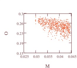
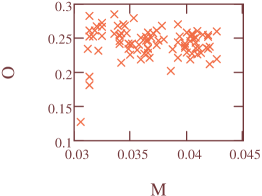
In each trial of set (a) a random input force sequence was applied at position $1$ (as described above). In each trial of set (b) no input sequence was applied. As is seen, the resulting behavior is clearly different in each of the two sets of trials. With an input present, as the complexity $M$ increases there appears to be a decreasing trend in the value of $O$ and an increase in the spread, i.e., the range of possible values of $O$. With no input, both $O$ and its spread of values are basically constant with respect to $M$.

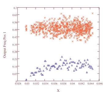
In Figure 2 we plot the frequency of $1$s in the output subsequence (this is the number of $1$s divided by the number of non-zero symbols in the output sequence).

Figure 2: Output frequeny of $1$s versus $M$

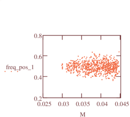
As can be seen, with an increase in the complexity there appears to be an increase in the spread of possible frequency values. Before we further discuss these results we proceed to perform the statistical tests.

5.1 Analysis

In order to test the significance of these results we estimate the output complexity O as a function of the complexity $M$. Denote by $X$ and $Y$ the random variables corresponding to $M$ and $O$, respectively. Let the underlying conditional probability distribution function be $P(Y|X)$ with marginals $P(X)$, $P(Y)$. As a sample we use the set of trials of Figure 1(a), denoted by $S=\left\{\left(x_{i},y_{i}\right)\right\}_{i=1}^{N}$ with cardinality $N=723$, and do linear regression in order to estimate $Y$ with dependence on $X$. Figure 3 shows the resulting estimate,

$$\hat{Y}(X)=0.341-2.284\,X,$$ (11)

surrounded by the $95\%$ confidence limits for the regression line, i.e., the actual regression line of the population falls within the limits defined by the two curved dashed lines.

Figure 3: Estimate for output complexity $Y$ as a function of complexity $X$

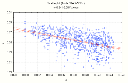
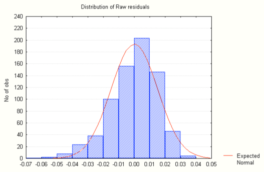
The following summarizes the accuracy of this linear regression estimate: $R^{2}=.246187335$ is the coeeficient of determination which measures the reduction in total variation of $Y$ due to $X$ and is defined as $R^{2}=1-(SS_{R}/SS)$ with $SS_{R}$ $=\sum_{i}\left(y_{i}-\hat{Y}(x_{i})\right)^{2}$ being the sum of squares of the residuals, $SS=\sum_{i}\left(y_{i}-\bar{y}\right)^{2}$ the total variation and $\bar{y}=\frac{1}{N}\sum_{i}y_{i}$ . The square root $R$ is the coeeficient of correlation between the independent variable $X$ and dependent variable $Y$. The standard error $SE=.015128505$ where $SE=\sqrt{\frac{1}{N}SS_{R}}$. Dividing $SS_{R}$ and $SS$ by their degrees of freedom and taking their ratio $F=SS/SS_{R}$ as an overall $F$ test gives $F(1,724)=236.4508$ which amounts to a $p$-value less than $0.000000$. Thus with very high confidence the residual variance differs from the total variation hence the linear estimate $\hat{Y}(X)$ explains well the variation of $Y$. The distribution of the residuals (shown in Figure 4) is very close to the normal distribution and the Durbin-Watson $d$ value is $1.994$ which implies that the assumptions on the residuals being uncorrelated and normaly distributed are met.

Figure 4: Distribution of the residuals $y_{i}-\hat{Y}(x_{i})$

Next, from Figure 1(a) it is evident that as the complexity $X$ increases the spread of the output complexity $Y$ increases. To quantify this assertion let us represent this spread by the random variable

$$Z(X,Y)=Y-\min_{y:P(y|X)>0}y.$$ (12)

As we have done above for $Y$ we now estimate $Z$ with dependence on $X$ (the model is shown only the value of $X$ and asked to predict $Z$). We form the following sample (based on $S$),

$$\zeta=\left\{\left(x_{i},z_{i}\right)\right\}_{i=1}^{N},\>z_{i}=y_{i}-\min_{x_{j}\in NN(x_{i},k)}y_{j}$$ (13)

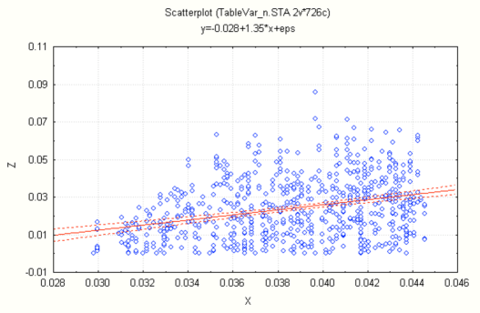
where $NN(x,k)$ denotes the set of $k$ nearest sample point $x_{j}$ to $x$ satisfying $x_{j}\leq x$. Figure 5 shows the resulting estimate equation (based on $k=7)$,

$$\hat{Z}(X)=-0.028+1.35\,X$$

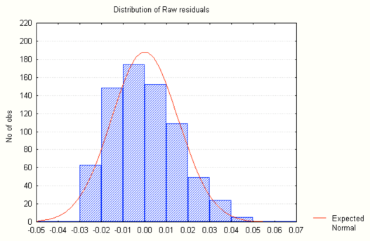
for the regression line. This verfies the increase in the value of $Z$ (i.e., in the spread of the output complexity $Y$) as the complexity $X$ increases. The following summarizes the accuracy of this regression estimate: $R^{2}=.098$, the $F$-ratio is $F(1,724)=79.548$ with a $p$-level smaller than $.000000$. The standard error of the estimate is $SE=.015413$ with a Durbin-Watson $d=1.938.$ Thus the estimator $\hat{Z}(X)$ accurately captures the variability of $Z$, i.e., the spread of output complexity $Y$. Figure 6 displays the distribution of the residuals.

Figure 5: Estimate of the spread in output complexity $Z$ as a function of the system’s complexity $X$

Figure 6: Distribution of residuals for $z_{i}-\hat{Z}(x_{i},y_{i})$

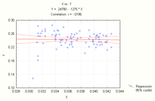
As mentioned above, Figure 1(b) shows that when no input is present the behavior of the output complexity is almost unaffected by the system’s complexity. To test this, we take the set of trials used in Figure 1(b) and study the correlation between the output complexity $Y$ and the system complexity $X$. As shown in Figure 7 there is hardly any correlation between them and the slope of the regression is almost zero.

Figure 7: The no-input scatter plot of output complexity $Y$ versus system’s complexity $X$

We already commented on the increasing spread of possible frequency values of the output subsequence (Figure 2) as the system’s complexity increases (with a random input sequence being applied). Denote by $Y$ the probability of having a $+1$ appear in the output subsequence and let $X$ be the system’s complexity. Let us define the following random variable

$$W(X)=\max_{y:P(y|X)>0}y-\min_{y:P(y|X)>0}y$$

to represent the spread in the possible values of the probability of $+1$. We form the following sample (based on $S$),

$$\zeta^{\prime}=\left\{\left(x_{i},w_{i}\right)\right\}_{i=1}^{N},\>w_{i}=\max_{x_{j}\in NN(x_{i},k)}y_{j}-\min_{x_{j}\in NN(x_{i},k)}y_{j}$$ (14)

with $k=7.$ Figure 8 shows (on the top scatter plot with red $\mathsf{x}$ symbols) the frequency of $1$s in the output subsequence versus the system complexity $X$. The bottom plot (with blue $\triangle$) shows the sample $\zeta^{\prime}$ with the $w$ component on the same vertical axis.

Figure 8: Scatter plot of frequency of $1$s in the output subsequence (top cluster of red $\mathsf{x}s$). The corresponding sample $\zeta^{\prime}$ used to estimate the spread $W$ as a function of the system’s complexity $X$ (bottom plot of blue $\triangle$)

We estimate $W$ based on $\zeta^{\prime}$ first transforming the $w_{i}$ values to $w_{i}^{2}$ and then doing linear regression to estimate $W^{2}$. Figure 9 shows the resulting estimate equation $-0.023+1.083\,X$ for $W^{2}$.

Figure 9: Estimate of the square of the spread $W^{2}$ of the output frequency of $1$s as a function of the system’s complexity $X$

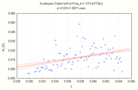
It follows that the estimate of $W$ is

$$\hat{W}(X)=\sqrt{1.083\,X-0.023}.$$ (15)

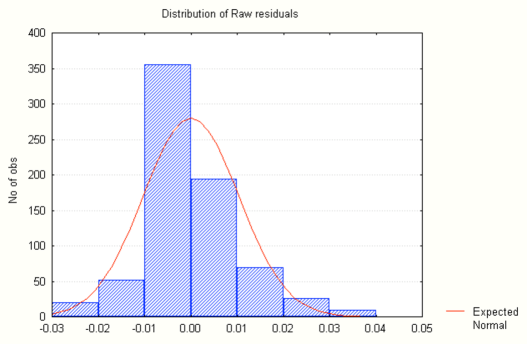
This verfies the increasing trend in the spread of values of the frequency of $1$s as the system’s complexity $X$ increases. The following summarizes the accuracy of this linear regression estimate: $R^{2}=.135$, the $F$-ratio is $F(1,724)=113.06$ with a $p$-level smaller than $.00000$. The standard error of the estimate is $SE=.01037$ and the Durbin-Watson $d=1.71$. The distribution of the residuals is shown in Figure 10.

Figure 10: Distribution of residuals $w_{i}^{2}-\hat{W^{2}}(x_{i})$

5.2 Some more details on the simulations

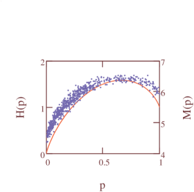
Several additional graphs showing additional details of the above experiments are shown below. Figure 11 shows the observed system description rate $M$ (scatter plot in blue) and the entropy (the minimal expected number of bits per character) used for the system description (red solid curve). They are plotted versus the probability parameter $p$ (in the range $0<p\leq 1)$ used to generate the random force sequence at position $15$ of the solid. It follows from the procedure (described above) of generating the system’s vibrating force that the entropy of the random variable $\mathcal{F}$ is $H(p)=-(1-p)\log(1-p)-p\log\frac{p}{2}.$ As seen from Figure 11, in order to get a higher system complexity one needs to draw a force sequence with a parameter $p$ closer to $\nicefrac{{1}}{{2}}$. There is some additional textual information ($145$ bytes) appended into each of the files that contain the $6200$-long ternary string that describes the system. Since $M$ is the ratio of the compressed to uncompressed versions (the actual uncompressed length as reported by the operating system is $6377$ bytes) then to get the rate for the number of bits per character used to describe the system (considering just the $145$-byte textual information and the $200$-byte force sequence at position $15$) we multiply $M$ by $6377\cdot 8$ and divide by $345$.

Figure 11: Entropy $H$ (red) v.s. observed system complexity $M$ (blue) as a function of parameter $p$ which represents the probability of having a non-zero (i.e. $\pm 1)$ symbol in the system’s vibrating force sequence (applied at position $15$)

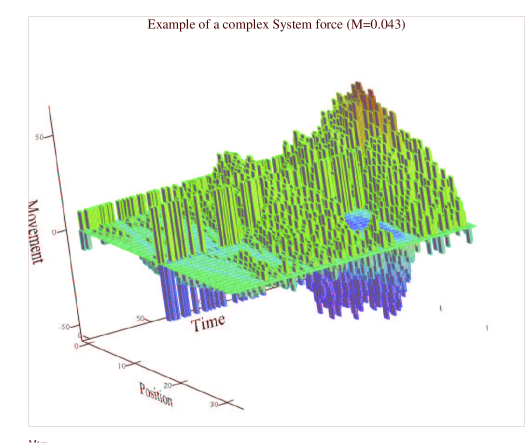
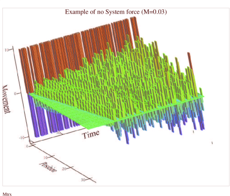
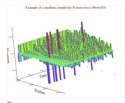
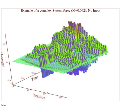
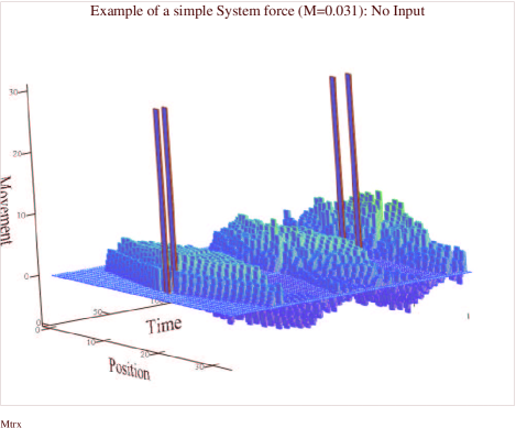
The next series of figures show examples of the actual solid’s response (displacement $u$ is shown on the $z$-axis) over time ($y$-axis) along the positions of the solid ($x$-axis). In all, the input sequence is maximally random with probability $\nicefrac{{1}}{{2}}$ for $+1$, $-1$. The magnitude of the input force sequence is $10$ and the magnitude of the system’s vibrating force sequence is $30$. The two force sequences are superimposed on the same 3D-plot that displays the displacement response. The output sequence is taken as the concatenation of the string obtained from the displacement at the last five positions (appearing on the plot to be closest to the reader). Figure 12 shows the response to a system of high complexity. Figure 13 shows a trial without a system force. This represents a low-complexity system. Figure 14 is the response of a system of a mid-level complexity. Figures 15 and 16 show the response when no input force is applied.

Figure 12: Response to a random input force sequence (applied at position 0). System’s vibrating force (at position 15) is of high complexity. Output is seen to be of low complexity.

Figure 13: Response to a random input force sequence (applied at position 0). System has no vibrating force applied hence is of minimal complexity. The output is seen to be of high complexity.

Figure 14: Response to a random input force sequence (applied at position 0). System’s vibrating force (at position 15) has a mid-level complexity. Output is seen to be of lower complexity than the example in Figure 13.

Figure 15: The no-input response to a system’s force (at position 15) of high complexity.

Figure 16: The no-input response to a system’s force (at position 15) of low complexity.

6 Conclusions

Based on these results, it is clear that when a random input sequence is applied to the vibrating solid (system) the observed output sequence is not simply a result of the random vibrating force sequence which is part of the system (applied at position 15) but is a direct consequence of the interaction of the system with an external random input force–when no input is present no significant correlation exists between the system and output complexities. The strong negative correlation between these two complexities (11) suggests that the system distorts the input randomness and produces a less complex output sequence. This agrees with the model introduced in [16] which says that a solid effectively acts as a selection rule picking bits from the input sequence to produce a less random output. This is evident in the significant decrease in the output complexity (Figure 3) and increase in its spread of values (Figure 5 ) indicating that the possibility of producing a less-complex output sequence increases as the system’s complexity rises.

The selected subsequence consists of $\pm 1$ with zeroes deleted. Being less chaotic, its stochastic level decreases. This is evident in the increase in the square of the spread of values of the frequency of $1$’s (Figure 9). The higher the system complexity, the higher the spread, i.e., the larger the bias from $\nicefrac{{1}}{{2}}$, the more the chance that the output sequence be less chaotic and random. If we divide the compressed length of the system by the length of the output (binary) subsequence and denote it by $X^{\prime}$ then re-estimate $W^{2}$ based on $X^{\prime}$ we obtain the following estimate for $W$,

$$\hat{W}(X^{\prime})=\sqrt{-0.03+0.173X^{\prime}}.$$ (16)

The $R^{2}=.0924$, $SE=.0106$, $F(1,724)=73.725$ and the p-level less than $0.00000$. The Durbin-Watson $d=1.66$. This estimate of the spread agrees with the rate predicted by the theory (2). To see this, let $x$ be the input sequence, let the system be the selection rule $R$ with a system complexity $K(R|n)$, let $R(x)$ be the output subsequence (consisting only of binary values $\pm 1$), let $\nu(R(x))$ be the frequency of $1$s in this subsequence and take the deficiency of randomness $\delta(x|n)$ of the input sequence to be zero (since the input sequence is maximally random). Then the theoretical rate of the maximal possible deviation (spread) between $\nu(R(x))$ and $\nicefrac{{1}}{{2}}$ is $O(\sqrt{K(R|n)/\ell(R(x))})$. This is the same rate in which the estimate of spread $W$ grows with respect to the $X^{\prime}$ in (16).

To summarize, the results above imply that a system based on classical equations of mechanics that consists of a vibrating solid subjected to external random input-force acts like an algorithmic selection rule of a finite complexity. It produces an output sequence whose stochastic and chaotic properties are effected by the system’s complexity as predicted by the theory of algorithmic randomness. The results confirm the model of [16].

References

- [1] A. E. Asarin. Some properties of Kolmogorov random finite sequences. SIAM Theory of Probability and its Applications, 32:507–508, 1987.
- [2] A. E. Asarin. On some properties of finite objects random in an algorithmic sense. Soviet Mathematics Doklady, 36(1):109–112, 1988.
- [3] L. Bienvenu. Kolmogorov-loveland stochasticity and kolmogorov complexity. In 24th Annual Symposium on Theoretical Aspects of Computer Science (STACS 2007), volume LNCS 4393, pages 260–271, 2007.
- [4] G. J. Chaitin. A theory of program size formally identical to information theory. Journal of the ACM, 22(3):329–340, 1975.
- [5] T. M. Cover and J. A. Thomas. Elements of Information Theory 2nd Edition (Wiley Series in Telecommunications and Signal Processing). Wiley-Interscience, July 2006.
- [6] B. Durand and N. Vereshchagin. Kolmogorov-Loveland stochasticity for finite strings. Information Processing Letters, 91(6):263–269, 2004.
- [7] P. Gacs. On the symmetry of algorithmic information. Soviet Mathematics Doklady, 15:1477–1480, 1974.
- [8] A. N. Kolmogorov. On tables of random numbers. Sankhyaa, The Indian Journal of Statistics, A(25):369–376, 1963.
- [9] A. N. Kolmogorov. Three approaches to the quantitative definition of information. Problems of Information Transmission, 1:1–17, 1965.
- [10] A. N. Kolmogorov. On tables of random numbers. Theoretical Computer Science, 207(2):387–395, 1998.
- [11] S. K. Lin. Correlation of entropy with similarity and symmetry. Journal of Chemical Information and Computer Sciences, 36:367–376, 1996.
- [12] S. K. Lin. The nature of the chemical process. 1. symmetry evolution - revised information theory, similarity principle and ugly symmetry. International Journal of Molecular Sciences., 2:10–39, 2001.
- [13] S. K. Lin. Gibbs paradox and the concepts of information, symmetry, similarity and their relationship. Entropy, 10:1–5, 2008.
- [14] D. W. Loveland. A new interpretation of the von Mises’ concept of random sequence. Zeitschrift fur mathematische Logik und Grundlagen der Mathematik, 12:279–294, 1966.
- [15] P. Martin-Lȯf. The definition of random sequences. Information and Control, 9:602–619, 1966.
- [16] J. Ratsaby. An algorithmic complexity interpretation of Lin’s third law of information theory. Entropy, 10(1):6–14, 2008.
- [17] C. P. Schnorr. A unified approach to the definition of random sequences. Mathematical Systems Theory, 5:246–258, 1971.
- [18] V.A. Uspenskil, A. L. Semenov, and A. Kh. Shen. Can and individual sequence of zeros and ones be random ? Russian Mathematical Surveys, 45(1):121–189, 1990.
- [19] V. V. Vyugin. Algorithmic complexity and stochastic properties of finite binary sequences. The Computer Journal, 42:294–317, 1999.
- [20] J. Ziv and A. Lempel. A universal algorithm for sequential data compression. IEEE Transactions on Information Theory, 23(3):337–343, 1977.