Asymptotic analysis and diffusion limit
of the Persistent Turning Walker Model

Abstract

The Persistent Turning Walker Model (PTWM) was introduced by Gautrais et al in Mathematical Biology for the modelling of fish motion. It involves a nonlinear pathwise functional of a non-elliptic hypo-elliptic diffusion. This diffusion solves a kinetic Fokker-Planck equation based on an Ornstein-Uhlenbeck Gaussian process. The long time “diffusive” behavior of this model was recently studied by Degond & Motsch using partial differential equations techniques. This model is however intrinsically probabilistic. In the present paper, we show how the long time diffusive behavior of this model can be essentially recovered and extended by using appropriate tools from stochastic analysis. The approach can be adapted to many other kinetic “probabilistic” models.

Keywords. Mathematical Biology; animal behavior; hypo-elliptic diffusions; kinetic Fokker-Planck equations; Poisson equation; invariance principles; central limit theorems, Gaussian and Markov processes.

AMS-MSC. 82C31; 35H10; 60J60; 60F17; 92B99; 92D50; 34F05.

1 Introduction

Different types of models are used in Biology to describe individual displacement. For instance, correlated/reinforced random walks are used for the modelling of ant, see e.g. [3, 25], and cockroaches, see e.g. [14] and [5] for a review. On the other hand, a lot of natural phenomena can be described by kinetic equations and their stochastic counterpart, stochastic differential equations. The long time behavior of such models is particularly relevant since it captures some “stationary” evolution. Recently, a new model, called the Persistent Turning Walker model (PTWM for short), involving a kinetic equation, has been introduced to describe the motion of fish [10, 6]. The natural long time behavior of this model is “diffusive” and leads asymptotically to a Brownian Motion.

The diffusive behavior of the PTWM has been obtained in [6] using partial differential equations techniques. In the present work, we show how to recover this result by using appropriate tools from stochastic processes theory. First, we indicate how the diffusive behavior arises naturally as a consequence of the Central Limit Theorem (in fact an Invariance Principle). As expected, the asymptotic process is a Brownian Motion in space. As a corollary, we recover the result of [6] which appears as a special case where the variance of the Brownian Motion can be explicitly computed. We finally extend our main result to more general initial conditions. We emphasize that the method used in the present paper is not restricted to the original PTWM. In particular, the hypotheses for the convergence enables to use more general kinetic models than the original PTWM.

The present paper is organized as follows: in Section 2, we recall the PTWM and its main properties, and we give the main results. Section 3 is dedicated to the proofs.

2 Main results

In the PTWM, the motion is described using three variables: position $x\in\mathbb{R}^{2}$, velocity angle $\theta\in\mathbb{R}$, and curvature $\kappa\in\mathbb{R}$. For some fixed real constant $\alpha$, the probability distribution $p(t,x,\theta,\kappa)$ of finding particles at time $t$ in a small neighborhood of $(x,\theta,\kappa)$ is given by a forward Chapman-Kolmogorov equation

$$\partial_{t}p+\tau.\nabla_{x}p+\kappa\partial_{\theta}p-\partial_{\kappa}(\kappa p)-\alpha^{2}\,\partial^{2}_{\kappa^{2}}p\,=\,0$$ (2.1)

with initial value $p_{0}$, where

$$\tau(\theta)=(\cos\theta,\sin\theta)=e^{\sqrt{-1}\,\theta}.$$

The stochastic transcription of (2.1) is given by the stochastic differential system $(t\geq 0)$

$$\begin{cases}dx_{t}=\tau(\theta_{t})\,dt\\ d\theta_{t}=\kappa_{t}\,dt\\ d\kappa_{t}=-\kappa_{t}\,dt\,+\,\sqrt{2}\alpha\,dB_{t}\end{cases}$$ (2.2)

where $(B_{t})_{t\geq 0}$ is a standard Brownian Motion on $\mathbb{R}^{2}$. The probability density function $p(t,x,\theta,\kappa)$ of $(x_{t},\theta_{t},\kappa_{t})$ with a given initial law $p_{0}\,dx\,d\theta\,d\kappa$ is then solution of (2.1). Also, (2.1) is in fact a kinetic Fokker-Planck equation. Note that $(\kappa_{t})_{t\geq 0}$ is an Ornstein-Uhlenbeck Gaussian process. The formula

$$\theta_{t}=\theta_{0}+\int_{0}^{t}\!\kappa_{s}\,ds$$

expresses $(\theta_{t})_{t\geq 0}$ as a pathwise linear functional of $(\kappa_{t})_{t\geq 0}$. In particular the process $(\theta_{t})_{t\geq 0}$ is Gaussian and is thus fully characterized by its initial value, together with its time covariance and mean which can be easily computed from the ones of $(\kappa_{t})_{t\geq 0}$ conditional on $\theta_{0}$ and $\kappa_{0}$. The process $(\theta_{t})_{t\geq 0}$ is not Markov. However, the pair $(\theta_{t},\kappa_{t})_{t\geq 0}$ is a Markov Gaussian diffusion process and can be considered as the solution of a degenerate stochastic differential equation, namely the last two equations of the system (2.2). Additionally, the process $(x_{t})_{t\geq 0}$ is an “additive functional” of $(\theta_{t},\kappa_{t})_{t\geq 0}$ since

$$x_{t}\ =\ x_{0}+\int_{0}^{t}\!\tau(\theta_{s})\,ds\ =\ x_{0}+\int_{0}^{t}\!\tau{{\left(\theta_{0}+\int_{0}^{s}\!\kappa_{u}\,du\right)}}\,ds.$$ (2.3)

Note that $x_{t}$ is a nonlinear function of $(\theta_{s})_{0\leq s\leq t}$ due to the nonlinear nature of $\tau$, and thus $(x_{t})_{t\geq 0}$ is not Gaussian. The invariant measures of the process $(\theta_{t},\kappa_{t})_{t\geq 0}$ are multiples of the tensor product of the Lebesgue measure on $\mathbb{R}$ with the Gaussian law of mean zero and variance $\alpha^{2}$. These measures cannot be normalized into probability laws. Since $\tau$ is $2\pi$-periodic, the process $(\theta_{t})_{t\geq 0}$ acts in the definition of $x_{t}$ only modulo $2\pi$, and one may replace $\theta$ by $\underline{\theta}\in S^{1}:=\mathbb{R}/2\pi\mathbb{Z}$. The Markov diffusion process

$${(y_{t})}_{t\geq 0}={(\underline{\theta}_{t},\kappa_{t})}_{t\geq 0}$$

has state space $S^{1}\times\mathbb{R}$ and admits a unique invariant law $\mu$ which is the tensor product of the uniform law on $S^{1}$ with the Gaussian law of mean zero and variance $\alpha^{2}$, namely

$$d\mu(\underline{\theta},\kappa)=\frac{1}{\sqrt{2\pi\alpha^{2}}}\mathds{1}_{S^{1}}(\underline{\theta})\exp{{\left(-\frac{\kappa^{2}}{2\alpha^{2}}\right)}}d\underline{\theta}d\kappa.$$

Note that ${(y_{t})}_{t\geq 0}$ is ergodic but is not reversible (this is simply due to the fact that the dynamics on observables depending only on $\underline{\theta}$ is not reversible). The famous Birkhoff-von Neumann Ergodic Theorem [16, 22, 13, 17, 7] states that for every $\mu$-integrable function $f:S^{1}\times\mathbb{R}\to\mathbb{R}$ and any initial law $\nu$ (i.e. the law of $y_{0}$), we have,

$$\mathbb{P}{{\left(\lim_{t\to\infty}{{\left(\frac{1}{t}\int_{0}^{t}\!f(y_{s})\,ds-\int_{S^{1}\times\mathbb{R}}\!f\,d\mu\right)}}=0\right)}}=1.$$ (2.4)

Beyond this Law of Large Numbers describing for instance the limit of the functional (2.3), one can ask for the asymptotic fluctuations, namely the long time behavior as $t\to\infty$ of

$$\sigma_{t}{{\left(\frac{1}{t}\int_{0}^{t}\!f(y_{s})\,ds-\int_{S^{1}\times\mathbb{R}}\!f\,d\mu\right)}}$$ (2.5)

where $\sigma_{t}$ is some renormalizing constant such that $\sigma_{t}\to\infty$ as $t\to\infty$. By analogy with the Central Limit Theorem (CLT for short) for reversible diffusion processes (see e.g. [9, 17]), we may expect, when $f$ is “good enough” and when $\sigma_{t}=\sqrt{t}$, a convergence in distribution of (2.5) as $t\to\infty$ to some Gaussian distribution with variance depending on $f$ and on the infinitesimal dynamics of ${(y_{t})}_{t\geq 0}$. This is the aim of Theorem 2.6 below, which goes actually further by stating a so called Invariance Principle, in other words a CLT for the whole process and not only for a fixed single time.

Theorem 2.6 (Invariance Principle at equilibrium).

Assume that $y_{0}=(\underline{\theta}_{0},\kappa_{0})$ is distributed according to the equilibrium law $\mu$. Then for any $C^{\infty}$ bounded $f:S^{1}\times\mathbb{R}\to\mathbb{R}$ with zero $\mu$-mean, the law of the process

$${(z_{t}^{\varepsilon})}_{t\geq 0}:={{\left(\varepsilon\int_{0}^{t/\varepsilon^{2}}\!\!\!\!f(y_{s})\,ds,\,y_{t/\varepsilon^{2}}\right)}}_{t\geq 0}$$

converges as $\varepsilon\to 0$ to $\mathcal{W}^{f}\otimes\mu^{\otimes\infty}$ where $\mathcal{W}^{f}$ is the law of a Brownian Motion with variance

$$V_{f}=-\int\!gLg\,d\mu=2\alpha^{2}\,\int\!|\partial_{\kappa}g|^{2}\,d\mu$$

where $L=\alpha^{2}\partial_{\kappa}^{2}-\kappa\partial_{\kappa}+\kappa\,\partial_{\theta}$ acts on $2\pi$-periodic functions in $\theta$, and $g:S^{1}\times\mathbb{R}\to\mathbb{R}$ is

$$g(y)=-\mathbb{E}\left(\int_{0}^{\infty}\!f(y_{s})\,ds\,\biggr{|}\,y_{0}=y\right).$$

In other words, for any fixed integer $k\geq 1$, any fixed times $0\leq t_{1}<\cdots<t_{k}$, and any bounded continuous function $F:(\mathbb{R}\times S^{1}\times\mathbb{R})^{k}\to\mathbb{R}$, we have

$$\lim_{\varepsilon\to 0}\mathbb{E}{{\left[F(z_{t_{1}}^{\varepsilon},\ldots,z_{t_{k}}^{\varepsilon})\right]}}=\mathbb{E}{{\left[F((W^{f}_{t_{1}},Y_{1}),\ldots,(W^{f}_{t_{k}},Y_{k}))\right]}}$$

where $Y_{1},\ldots,Y_{k}$ are independent and equally distributed random variables of law $\mu$ and where ${(W_{t}^{f})}_{t\geq 0}$ is a Brownian Motion with law $\mathcal{W}^{f}$, independent of $Y_{1},\ldots,Y_{k}$.

Theorem 2.6 encloses some decorrelation information as $\varepsilon$ goes to $0$ since the limiting law is a tensor product (just take for $F$ a tensor product function). Such a convergence in law at the level of the processes expresses a so called Invariance Principle. Here the Invariant Principle is at equilibrium since $y_{0}$ follows the law $\mu$. The proof of Theorem 2.6 is probabilistic, and relies on the fact that $g$ solves the Poisson equation $Lg=f$. Note that neither the reversible nor the sectorial assumptions of [9] are satisfied here.

Theorem 2.6 remains valid when $f$ is complex valued (this needs the computation of the asymptotic covariance of the real and the imaginary part of $f$). The hypothesis on $f$ enables to go beyond the original framework of [6]. For instance, we could add the following rule in the model: the speed of the fish decreases as the curvature increases. Mathematically, this is roughly translated as:

$$f(y)=f(\theta,\kappa)=c(|\kappa|)(\cos\theta,\,\sin\theta)$$ (2.7)

where $s\mapsto c(s)$ is a regular enough decreasing function, see Figure 1 for a simulation.

Figure 1: An example of the trajectory $t\mapsto x_{t}=(x_{t}^{1},x_{t}^{2})$ of the PTWM where the speed of the fish decreases with higher curvature (eq. 2.7). Here $\alpha=1$ and $c(|\kappa|)=1/(1+2|\kappa|)$. The simulation is run during 10 time units, we plot a point each $.1$ time unit.

The following corollary is obtained from Theorem 2.6 by taking roughly $f=\tau$ and by computing $V_{\tau}$ explicitly. In contrast with the function $f$ in Theorem 2.6, the function $\tau$ is complex valued. Also, an additional argument is in fact used in the proof of Corollary 2.8 to compute the asymptotic covariance of the real and imaginary parts of the additive functional based on $\tau$ (note that this seems to be missing in [6]).

Corollary 2.8 (Invariance Principle for PTWM at equilibrium).

Assume that the initial value $y_{0}=(\underline{\theta}_{0},\kappa_{0})$ is distributed according to the equilibrium $\mu$. Then the law of the process

$${{\left(\varepsilon\int_{0}^{t/\varepsilon^{2}}\!\!\!\!\tau(\theta_{s})\,ds,\,y_{t/\varepsilon^{2}}\right)}}_{t\geq 0}$$ (2.9)

converges as $\varepsilon\to 0$ to $\mathcal{W}^{\tau}\otimes\mu^{\otimes\infty}$ where $\mathcal{W}^{\tau}$ is the law of a $2$-dimensional Brownian Motion with covariance matrix $\mathbb{D}I_{2}$ where

$$\mathbb{D}=\int_{0}^{\infty}\!e^{-\,\alpha^{2}(s-1+e^{-s})}\,ds.$$

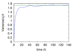
Figure 2: Convergence of $t^{-1}\mathrm{Var}(x_{t})$ to the constant $\mathbb{D}$. Here $\alpha=1$.

It can be shown that the constant $\mathbb{D}$ which appears in Corollary 2.8 satisfies to

$$\mathbb{D}=\lim_{t\to\infty}\frac{1}{t}\mathrm{Var}(x_{t}^{1})=\lim_{t\to\infty}\frac{1}{t}\mathrm{Var}(x_{t}^{2})\quad\text{where}\quad(x_{t}^{1},x_{t}^{2})=x_{t}=\int_{0}^{t}\!\!\!\tau(\theta_{s})\,ds$$

see e.g. Figure 2. Corollary 2.8 complements a result of Degond & Motsch [6, Theorem 2.2] which states – in their notations – that the probability density function

$$p^{\varepsilon}(t,x,\underline{\theta},\kappa)=\frac{1}{\varepsilon^{2}}\,p\,\left(\frac{t}{\varepsilon^{2}},\frac{x}{\varepsilon},\underline{\theta},\kappa\right)$$

converges as $\varepsilon\to 0$ to the probability density

$$\frac{1}{\sqrt{2\pi}}\,n^{0}(t,x)\,M(\kappa)$$

where $M$ is the Gaussian law with zero mean and variance $\alpha^{2}$, and $n^{0}$ solves the equation

$$\partial_{t}n^{0}-\frac{1}{2}\mathbb{D}\Delta_{x}n^{0}=0$$

where $\mathbb{D}$ is as in Corollary 2.8. Convergence holds in a weak sense in some well chosen Banach space, depending on the initial distribution. The meaning of $p^{\varepsilon}$ is clear from the stochastic point of view: it is the probability density function of the distribution of the rescaled process (recall that $x$ is two-dimensional)

$${{\left(\varepsilon x_{t/\varepsilon^{2}},\,y_{t/\varepsilon^{2}}\right)}}_{t\geq 0}={{\left(\varepsilon x_{t/\varepsilon^{2}},\ \underline{\theta}_{t/\varepsilon^{2}},\ \kappa_{t/\varepsilon^{2}}\right)}}_{t\geq 0}.$$

In other words, the main result of [6] captures the asymptotic behavior at fixed time of the process (2.9) by stating that for any $t$, and as $\varepsilon\to 0$, the law of this process at time $t$ tends to the law of $(\sqrt{\mathbb{D}}W_{t},\underline{\theta},M)$ where $(W_{t})_{t\geq 0}$, and $(\underline{\theta},M)$ are independent, $(W_{t})_{t\geq 0}$ being a standard Brownian Motion, and $(\underline{\theta},M)$ a random variable following the law $\mu$. This result encompasses what is expected by biologists i.e. a “diffusive limiting behavior”.

Starting from the equilibrium, Corollary 2.8 is on one hand stronger and on the other hand weaker than the result of [6] mentioned above. Stronger because it is relative to the full law of the process, not only to each marginal law at fixed time $t$. In particular it encompasses covariance type estimates at two different times. Weaker because it is concerned with the law and not with the density. For the density at time $t$ we recover a weak convergence, while the one obtained in [6] using partial differential equations techniques is of strong nature. We should of course go further using what is called “local CLTs”, dealing with densities instead of laws, but this will require some estimates which are basically the key of the analytic approach used in [6].

Our last result concerns the behavior when the initial law is not the invariant law $\mu$.

Theorem 2.10 (Invariance Principle out of equilibrium).

The conclusion of Corollary 2.8 still holds true when $y_{0}=(\underline{\theta}_{0},\kappa_{0})$ is distributed according to some law $\nu$ such that $d\nu_{s_{0}}/d\mu$ belongs to $\mathbb{L}^{q}(\mu)$ for some $s_{0}\geq 0$ and $q>1$, where $\nu_{s_{0}}$ is the law of $y_{s_{0}}$. This condition is fulfilled for instance if $d\nu/d\mu$ belongs to $\mathbb{L}^{q}(\mu)$ or if $\nu$ is compactly supported.

3 Proofs

The story of CLTs and Invariant Principles for Markov processes is quite intricate and it is out of reach to give a short account of the literature. The reader may find however a survey on some aspects in e.g. [9, 15, 27, 17]. Instead we shall exhibit some peculiarities of our model that make the long time study an (almost) original problem. The underlying diffusion process $(\theta_{t},\kappa_{t})_{t\geq 0}$ with state space $\mathbb{R}^{2}$ is degenerate in the sense that its infinitesimal generator

$$L=\alpha^{2}\,\partial^{2}_{\kappa^{2}}\,-\,\kappa\,\partial_{\kappa}\,+\,\kappa\,\partial_{\theta}$$ (3.1)

is not elliptic. Fortunately, the operator $\partial_{t}+L$ is Hörmander hypo-elliptic since the “diffusion” vector field $X=(0,\alpha^{2})$ and the Lie bracket $[X,Y]=XY-YX$ of $X$ with the “drift” vector field $Y=(\kappa,-\kappa)$ generate the full tangent space at each $(\theta,\kappa)\in\mathbb{R}^{2}$. The drift vector field $Y$ is always required, so that the generator is “fully degenerate”. This degeneracy of $L$ has two annoying consequences:

1. any invariant measure $\nu$ of $L$ is not symmetric, i.e. $\int\!fLg\,d\nu\neq\int\!gLf\,d\nu$ for some nice functions $f$ and $g$ in $\mathbb{L}^{2}(\nu)$, for instance only depending on $\theta$.

2. the carré du champ of $L$ given here by $\Gamma f=\frac{1}{2}L(f^{2})-fLf=2\alpha^{2}|\partial_{\kappa}f|^{2}$ is degenerate, so that one cannot expect to use any usual functional inequality such as the Poincaré inequality (i.e. spectral gap, see [1, 23]) in order to study the long time behavior.

This situation is typical for kinetic models. In the more general framework of homogenization, a slightly more general version of this model has been studied in [11], see also the trilogy [19, 20, 21] for similar results from which one can derive the result in [6]. The main ingredient of the proof of Theorem 2.6 is the control of the “rate of convergence” to equilibrium in the Ergodic Theorem (2.4), for the process $(\underline{\theta}_{t},\kappa_{t})_{t\geq 0}$. We begin with a simple lemma which expresses the propagation of chaos as $\varepsilon$ goes to $0$.

Lemma 3.2 (Propagation of chaos).

Assume that $y_{0}=(\underline{\theta}_{0},\kappa_{0})$ is distributed according to the equilibrium law $\mu$. Then the law of the process $(y^{\varepsilon})_{t\geq 0}={{\left(y_{t/\varepsilon^{2}}\right)}}_{t\geq 0}$ converges as $\varepsilon\to 0$ to $\mu^{\otimes\infty}$. In other words, for any fixed integer $k\geq 1$, any fixed times $0\leq t_{1}<\cdots<t_{k}$, and any bounded continuous function $F:(S^{1}\times\mathbb{R})^{k}\to\mathbb{R}$, we have

$$\lim_{\varepsilon\to\infty}\mathbb{E}{{\left[F(y_{t_{1}}^{\varepsilon},\ldots,y_{t_{k}}^{\varepsilon})\right]}}=\mathbb{E}{{\left[F(Y_{1},\ldots,Y_{k})\right]}}$$

where $Y_{1},\ldots,Y_{k}$ are independent and equally distributed random variables of law $\mu$.

Proof of Lemma 3.2.

Let us denote by $L$ the operator (3.1) acting this time on $2\pi$-periodic functions in $\theta$, i.e. on functions $S^{1}\times\mathbb{R}\to\mathbb{R}$. This operator $L$ generates a non-negative contraction semi-group $(P_{t})_{t\geq 0}=(e^{tL})_{t\geq 0}$ in $\mathbb{L}^{2}(\mu)$ with the stochastic representation $P_{t}f(y)=\mathbb{E}[f(y_{s})|y_{0}=y]$ for all bounded $f$. We denote by $L^{*}$ the adjoint of $L$ in $\mathbb{L}^{2}(\mu)$ generating the adjoint semi-group $P_{t}^{*}$, i.e.

$$L^{*}=\alpha^{2}\partial^{2}_{\kappa}-\kappa\partial_{\kappa}-\kappa\partial_{\theta}$$

acting again on the same functions. The function $H(y)=H(\underline{\theta},\kappa)=1+\kappa^{2}$ satisfies

$$L^{*}H=-2H+2(\alpha^{2}+1)\leq-H+2(\alpha^{2}+1)\,\mathds{1}_{|\kappa|\leq\sqrt{2\alpha^{2}+1}}$$ (3.3)

so $H$ is a Lyapunov function in the sense of [2, Def. 1.1]. Since $C=S^{1}\times\{|\kappa|\leq\sqrt{2\alpha^{2}+1}\}$ is compact and the process $(y_{t})_{t\geq 0}$ is regular enough, $C$ is a “petite set” in the terminology [2, Def. 1.1] of Meyn & Tweedie. Accordingly we may apply [2, Th. 2.1] and conclude that there exists a constant $K_{2}>0$ such that for all bounded $f$ satisfying $\int fd\mu=0$,

$${{\left\|P_{t}f\right\|}}_{\mathbb{L}^{2}(\mu)}\leq K_{2}\,{{\left\|f\right\|}}_{\infty}e^{-t}.$$ (3.4)

We shall give a proof of the Lemma for $k=2$, the general case $k\geq 2$ being heavier but entirely similar. We set $s=t_{1}<t_{2}=t$. It is enough to show that for every bounded continuous functions $F,G:S^{1}\times\mathbb{R}\to\mathbb{R}$, we have the convergence

$$\lim_{\varepsilon\to 0}\mathbb{E}[F(y_{s}^{\varepsilon})G(y_{t}^{\varepsilon})]=\mathbb{E}[F(Y)]\mathbb{E}[G(Y)]$$

where $Y$ is a random variable of law $\mu$. Since $y_{0}$ follows the law $\mu$, we can safely assume that the functions $F$ and $G$ have zero $\mu$-mean, and reduce the problem to show that

$$\mathbb{E}[F(y_{s}^{\varepsilon})G(y_{t}^{\varepsilon})]=\int\!P_{s/\varepsilon^{2}}(FP_{(t-s)/\varepsilon^{2}}G)\,d\mu=\int\!FP_{(t-s)/\varepsilon^{2}}G\,d\mu\underset{\varepsilon\to 0}{\longrightarrow}0.$$

Now since $\mu$ is a probability measure, we have $\mathbb{L}^{2}(\mu)\subset\mathbb{L}^{1}(\mu)$ and thus

$${{\left|\int\!FP_{(t-s)/\varepsilon^{2}}G\,d\mu\right|}}\leq{{\left\|FP_{(t-s)/\varepsilon^{2}}G\right\|}}_{1}\leq{{\left\|FP_{(t-s)/\varepsilon^{2}}G\right\|}}_{2}\leq{{\left\|F\right\|}}_{\infty}{{\left\|P_{(t-s)/\varepsilon^{2}}G\right\|}}_{2}.$$

The desired result follows then from the $\mathbb{L}^{2}-\mathbb{L}^{\infty}$ bound (3.4) since

$${{\left\|P_{(t-s)/\varepsilon^{2}}G\right\|}}_{\mathbb{L}^{2}(\mu)}\leq K_{2}{{\left\|G\right\|}}_{\infty}e^{-(t-s)/\varepsilon^{2}}\underset{\varepsilon\to 0}{\longrightarrow}0.$$

∎

Proof of Theorem 2.6.

The strategy is the usual one based on Itô’s formula, Poisson equation, and a martingale CLT. However, each step involves some peculiar properties of the stochastic process. For convenience we split the proof into small parts with titles.

Poisson equation

Let $L$, $L^{*}$, and $(P_{t})_{t\geq 0}$ be as in the proof of Lemma 3.2. Since $f$ is bounded and satisfies $\int fd\mu=0$ (i.e. $f$ has zero $\mu$-mean), the bound (3.4) ensures that

$$g=-\int_{0}^{\infty}\!P_{s}f\,ds\quad\in\mathbb{L}^{2}(\mu).$$

Furthermore, the formula $P_{t}g-g=\int_{0}^{t}\,P_{s}f\,ds$ ensures that

$$\lim_{t\to 0}\frac{1}{t}(P_{t}g-g)=f\quad\text{strongly in $\mathbb{L}^{2}(\mu)$.}$$

It follows that $g$ belongs to the $\mathbb{L}^{2}(\mu)$-domain of $L$ and satisfies to the Poisson equation:

$$Lg=f\quad\text{in $\mathbb{L}^{2}(\mu)$}.$$

Since $\mu$ has an everywhere positive density with respect to the Lebesgue measure on $S^{1}\times\mathbb{R}$, we immediately deduce that $g$ belongs to the set of Schwartz distributions $\mathcal{D}^{\prime}$ and satisfies $Lg=f$ in this set. Since $L$ is hypo-elliptic (it satisfies the Hörmander brackets condition) and $f$ is $C^{\infty}$, it follows that $g$ belongs to $C^{\infty}$. Hence we have solved the Poisson equation $Lg=f$ in a strong sense. Remark that since $g\in\mathbb{L}^{2}(\mu)$ and $f$ is bounded, we get

$$\mathbb{E}_{\mu}[2\alpha^{2}\,|\partial_{\kappa}\,g|^{2}]=-\mathbb{E}_{\mu}[gLg]=-\mathbb{E}_{\mu}[gf]<\infty.$$

Itô’s formula

Since $g$ is smooth, we may use Itô’s formula to get

$$g(y_{t})-g(y_{0})=\int_{0}^{t}\!\alpha\sqrt{2}\,\partial_{\kappa}g(y_{s})\,dB_{s}+\int_{0}^{t}\!Lg(y_{s})\,ds\quad\text{almost surely}$$

which can be rewritten thanks to the Poisson equation $Lg=f$ as

$$\int_{0}^{t}\!f(y_{s})\,ds=g(y_{t})-g(y_{0})-\alpha\sqrt{2}\int_{0}^{t}\!\partial_{\kappa}g(y_{s})\,dB_{s}\quad\text{almost surely}.$$ (3.5)

This last equation (3.5) reduces the CLT for the process

$${{\left(\varepsilon\int_{0}^{t/\varepsilon^{2}}\!f(y_{s})\,ds\right)}}_{t\geq 0}$$

to showing that $(\varepsilon(g(y_{t/\varepsilon^{2}})-g(y_{0})))_{t\geq 0}$ goes to zero as $\varepsilon\to 0$ and to a CLT for the process

$${{\left(\alpha\varepsilon\sqrt{2}\int_{0}^{t/\varepsilon^{2}}\!\partial_{\kappa}g(y_{s})\,dB_{s}\right)}}_{t\geq 0}.$$

For such, we shall use the initial conditions and a martingale argument respectively.

Initial condition

Since the law $\mu$ of $y_{0}$ is stationary, Markov’s inequality gives for any constant $K>0$,

$$\mathbb{P}(|g(y_{t/\varepsilon^{2}})|\geq K/\varepsilon)=\mathbb{P}(|g(y_{0})|\geq K/\varepsilon)\leq\frac{\mathrm{Var}_{\mu}(g)\,\varepsilon^{2}}{K^{2}}\underset{\varepsilon\to 0}{\longrightarrow}0.$$

It follows that any n-uple of increments

$$\varepsilon\,(g(y_{t_{1}})-g(y_{t_{0}}),\ldots,g(y_{t_{n}})-g(y_{t_{n-1}}))$$

converges to $0$ in probability as $\varepsilon\to 0$. Thanks to (3.5), this reduces the CLT for

$${{\left(\varepsilon\int_{0}^{t/\varepsilon^{2}}\!f(y_{s})\,ds\right)}}_{t\geq 0}$$

to the CLT for

$$(M_{t}^{\varepsilon})_{t\geq 0}:={{\left(\varepsilon\alpha\sqrt{2}\int_{0}^{t/\varepsilon^{2}}\!\partial_{\kappa}g(y_{s})\,dB_{s}\right)}}_{t\geq 0}.$$

Martingale argument

It turns out that $((M_{t}^{\varepsilon})_{t\geq 0})_{\varepsilon>0}$ is a family of local martingales. These local martingales are actually $\mathbb{L}^{2}$ martingales whose brackets (increasing processes)

$${{\left<M^{\varepsilon}\right>}}_{t}=\varepsilon^{2}2\alpha^{2}\int_{0}^{t/\varepsilon^{2}}\!|\partial_{\kappa}g|^{2}(y_{s})\,ds$$

converge almost surely to

$$2\alpha^{2}t\mathbb{E}_{\mu}[|\partial_{\kappa}\,g|^{2}]=t\,V_{f}\quad\text{as $\varepsilon\to 0$}$$

thanks to the Ergodic Theorem (2.4). According to the CLT for $\mathbb{L}^{2}$-martingales due to Rebolledo, see for example [12] for an elementary proof, it follows that the family $(M_{t}^{\varepsilon})_{t\geq 0}$ converges weakly (for the Skorohod topology) to $V_{f}\,(B_{t}^{\tau})_{t\geq 0}$ where $(B_{t}^{\tau})_{t\geq 0}$ is a standard Brownian Motion. Consequently, we obtain the desired CLT for the process

$${{\left(\varepsilon\int_{0}^{t/\varepsilon^{2}}\!\!\!\!f(y_{s})\,ds\right)}}_{t\geq 0}.$$

Namely, its increments are converging in distribution as $\varepsilon\to 0$ to the law of a Brownian Motion with variance $V_{\tau}$. It remains to obtain the desired CLT for the process ${(z_{t}^{\varepsilon})}_{t\geq 0}$.

Coupling with propagation of chaos and asymptotic independence

By the result above and Lemma 3.2, the CLT for ${(z_{t}^{\varepsilon})}_{t\geq 0}$ will follow if we show that

$${{\left(\varepsilon\int_{0}^{t/\varepsilon^{2}}\!\!\!\!f(y_{s})\,ds\right)}}_{t\geq 0}\quad\text{and}\quad(y_{t/\varepsilon^{2}})_{t\geq 0}={(\underline{\theta}_{t/\varepsilon^{2}},\kappa_{t/\varepsilon^{2}})}_{t\geq 0}$$

are independent processes as $\varepsilon\to 0$. It suffices to establish the independence as $\varepsilon\to 0$ for an arbitrary $k$-uple of times $0=t_{0}<t_{1}<\cdots<t_{k}=t$. To this end, let us introduce a bounded continuous function $h$ and the smooth bounded functions

$$h_{j}(u)=e^{\sqrt{-1}b_{j}u}$$

where $1\leq j\leq k$ for given real numbers $b_{1},\ldots,b_{k}$. Let us define

$$A^{\varepsilon}=\mathbb{E}_{\mu}{{\left[h(y_{t/\varepsilon^{2}})\prod_{j=1}^{k}h_{j}{{\left(\varepsilon\int_{t_{j-1}/\varepsilon^{2}}^{t_{j}/\varepsilon^{2}}\,f(y_{s})\,ds\right)}}\right]}}$$

Introduce $t_{\varepsilon}=(t/\varepsilon^{2})-(t/\sqrt{\varepsilon})$ and $s_{\varepsilon}=t/\sqrt{\varepsilon}$. For $\varepsilon$ small enough, $t_{\varepsilon}>(t_{k-1}\varepsilon^{2})$, so that using the Markov property at time $t_{\varepsilon}$ we get

$$A^{\varepsilon}=\mathbb{E}_{\mu}{{\left[\prod_{j=1}^{k-1}h_{j}{{\left(\varepsilon\int_{t_{j-1}/\varepsilon^{2}}^{t_{j}/\varepsilon^{2}}\!f(y_{s})\,ds\right)}}\mathbb{E}_{\mu}{{\left[h(y_{t/\varepsilon^{2}})h_{k}{{\left(\varepsilon\int_{t_{k-1}/\varepsilon^{2}}^{t_{k}/\varepsilon^{2}}\!f(y_{s})\,ds\right)}}\,\biggr{|}\,\mathcal{F}_{t_{\varepsilon}}\right]}}\right]}}$$

The conditional expectation in the right hand side is equal to

$$h_{k}{{\left(\varepsilon\int_{t_{k-1}/\varepsilon^{2}}^{t_{\varepsilon}}\!f(y_{s})\,ds\right)}}\mathbb{E}{{\left[h(y_{s_{\varepsilon}})h_{k}{{\left(\varepsilon\int_{0}^{s_{\varepsilon}}\!f(y_{s})\,ds\,\biggr{|}\,y_{0}=y_{t_{\varepsilon}}\right)}}\right]}}$$

and the second term can be replaced by

$$\mathbb{E}{{\left[h(y_{s_{\varepsilon}})\,\biggr{|}\,y_{0}=y_{t_{\varepsilon}}\right]}}$$

up to an error less than

$$\varepsilon{{\left\|h\right\|}}_{\infty}{{\left\|f\right\|}}_{\infty}s_{\varepsilon}$$

going to $0$ as $\varepsilon\to 0$. It thus remains to study

$$\mathbb{E}_{\mu}{{\left[\prod_{j=1}^{k-1}h_{j}{{\left(\varepsilon\int_{t_{j-1}/\varepsilon^{2}}^{t_{j}/\varepsilon^{2}}\!f(y_{s})\,ds\right)}}h_{k}{{\left(\varepsilon\int_{t_{k-1}/\varepsilon^{2}}^{t_{\varepsilon}}\!f(y_{s})\,ds\right)}}\mathbb{E}{{\left[h(y_{s_{\varepsilon}})\,\biggr{|}\,y_{0}=y_{t_{\varepsilon}}\right]}}\right]}}.$$

Conditioning by $y_{t_{\varepsilon}}$, this can be written in the form

$$\int\,H(\varepsilon,y)\,P_{s_{\varepsilon}}h(y)\,\mu(dy)$$

with a bounded $H$, so that using the convergence of the semi-group, we may again replace $P_{s_{\varepsilon}}h$ by $\int hd\mu$ up to an error term going to $0$. It remains to apply the previously obtained CLT in order to conclude to the convergence and asymptotic independence. ∎

Remark 3.6 (More general models).

The proof of Theorem 2.6 immediately extends to more general cases. The main point is to prove that $g$ solves the Poisson equation in $\mathbb{L}^{2}(\mu)$. In particular it is enough to have an estimate of the form

$${{\left\|P_{t}f\right\|}}_{\mathbb{L}^{2}(\mu)}\leq\alpha(t)\,{{\left\|f\right\|}}_{\infty}$$

for every $t\geq 0$ with a function $\alpha$ satisfying

$$\int_{0}^{\infty}\!\alpha(s)\,ds<\infty.$$

According to [2], a sufficient condition for this to hold is to find a smooth increasing positive concave function $\varphi$ such that the function $\alpha$ defined by

$$\alpha(t)=\frac{1}{(\varphi\circ G_{\varphi}^{-1})(t)}\quad\text{where}\quad G_{\varphi}(u)=\int_{1}^{u}\!\frac{1}{\varphi(s)}\,ds$$

satisfies the integrability condition above, and a Lyapunov function $H\geq 1$ such that

$$\int\!H\,d\mu<\infty\quad\text{and}\quad L^{*}H\leq-\varphi(H)+O(\mathds{1}_{C})$$

for some compact subset $C$. In particular we may replace the Ornstein-Uhlenbeck dynamics for $\kappa$ by a more general Kolmogorov diffusion dynamics of the form

$$d\kappa_{t}=-\nabla V(\kappa_{t})dt+\sqrt{2}\,dB_{t}.$$

The invariant measure of $(\kappa_{t},\theta_{t})_{t\geq 0}$ is then $e^{-V(\kappa)}d\kappa d\theta$. We refer for instance to [8, 2] for the construction of Lyapunov functions in this very general situation. For example, in one dimension, one can take $V^{\prime}(x)=|x|^{p}$ for large $|x|$ and $0<p\leq 1$. Choosing $H(y)=|\kappa|^{q}$ for large $\kappa$ furnishes a polynomial decay of any order by taking $q$ as large as necessary. Actually, in this last situation, the decay rate is sub–exponential, see for example [8, 2].

Remark 3.7 (Asymptotic covariance).

It is worth noticing that if the asymptotic variance

$$(AV)_{f}=\lim_{t\to\infty}\,\frac{1}{t}\,\mathbb{E}_{\mu}{{\left[{{\left(\int_{0}^{t}\!f(y_{s})\,ds\right)}}^{2}\right]}}$$

exists, then $V_{f}=(AV)_{f}$. Similarly we may consider complex valued functions $f$ and replace the asymptotic variance by the asymptotic covariance matrix which takes into account the variances and the covariance of the real and imaginary parts of $f$.

Proof of Corollary 2.8.

We may now apply the previous theorem and the previous remark to the $2$-dimensional smooth and $\mu$-centered function $\tau$. The only thing we have to do is to compute the asymptotic covariance matrix. To this end, first remark that elementary Gaussian computations furnishes the following explicit expressions

$$\kappa_{t} =e^{-t}\,\kappa_{0}+\sqrt{2}\,\alpha\,\int_{0}^{t}\,e^{s-t}\,dB_{s}\,,$$ (3.8)

$$\theta_{t} =\theta_{0}+(1-e^{-t})\,\kappa_{0}+\sqrt{2}\,\alpha\,\int_{0}^{t}\,(1-e^{s-t})\,dB_{s}\,.$$ (3.9)

Since $x_{t}^{1}=\int_{0}^{t}\,\cos\theta_{s}\,ds$ and $x_{t}^{2}=\int_{0}^{t}\,\sin\theta_{s}\,ds$, Markov’s property and stationarity yield

$$\mathbb{E}_{\mu}[x_{t}^{1}\,x_{t}^{2}] =\mathbb{E}_{\mu}{{\left[\int_{0}^{t}\!(x_{s}^{1}\sin\theta_{s}+x_{s}^{2}\cos\theta_{s})\,ds\right]}}$$ (3.10)

$$=\mathbb{E}_{\mu}{{\left[\int_{0}^{t}\!\int_{0}^{s}\!(\cos\theta_{u}\sin\theta_{s}+\sin\theta_{u}\cos\theta_{s})\,du\,ds\right]}}$$

$$=\int_{0}^{t}\!\int_{0}^{s}\!\mathbb{E}_{\mu}[\sin(\theta_{u}+\theta_{s})]\,du\,ds$$

$$=\int_{0}^{t}\!\int_{0}^{s}\!\mathbb{E}_{\mu}{{\left[\sin{{\left(2\theta_{0}+2(1-e^{u-s})\kappa_{0}+\sqrt{2}\alpha\int_{0}^{s-u}\!(1-e^{v-(s-u)})\,dB^{\prime}_{v}\right)}}\right]}}\,du\,ds$$

where $(B^{\prime}_{t})_{t\geq 0}$ is a Brownian Motion independent of $(\kappa_{0},\underline{\theta}_{0})$. Since $\kappa_{0}$ and $\underline{\theta}_{0}$ are also independent (recall that $\mu$ is a product law), we may first integrate with respect to $\underline{\theta}_{0}$ (fixing the other variables), i.e. we have to calculate $\mathbb{E}_{\mu}(\sin(2\underline{\theta}_{0}+C))$ which is equal to $0$ since the law $\mu$ of $\underline{\theta}_{0}$ is uniform on $[0,2\pi[$. Hence the $\mu$-covariance of $(x_{t}^{1},x_{t}^{2})$ is equal to $0$ (since this is a Gaussian process, both variables are actually independent), and similar computations show that the asymptotic covariance matrix is thus $\mathbb{D}I_{2}$ where

$$\mathbb{D}=\int_{0}^{\infty}\!e^{-\,\alpha^{2}(s-1+e^{-s})}\,ds.$$

∎

Proof of Theorem 2.10.

We assume now that $y_{0}\sim\nu$ instead of $y_{0}\sim\mu$. We may mimic the proof of Theorem 2.6, provided we are able to control $\mathbb{E}_{\nu}(g^{2}(y_{s}))$. Indeed the invariance principle for the local martingales $(M_{t}^{\varepsilon})_{t\geq 0}$ is still true for the finite-dimensional convergence in law, according for instance to [13, Th. 3.6 p. 470]. The Ergodic Theorem ensures the convergence of the brackets. The first remark is that these controls are required only for $s\geq s_{0}\geq 0$ where $s_{0}$ is fixed but arbitrary. Indeed since $\tau$ is bounded, the quantity

$$\varepsilon\int_{0}^{s_{0}}\!\tau(\theta_{s})\,ds$$

goes to $0$ almost surely, so that we only have to deal with $\int_{s_{0}}^{t/\varepsilon^{2}}$ so that we may replace $0$ by $s_{0}$ in all the previous derivation. Thanks to the Markov property we thus have to control $\mathbb{E}_{\nu_{s_{0}}}(g^{2}(y_{s}))$ for all $s>0$, where $\nu_{s_{0}}$ denote the law of $y_{s_{0}}$. This remark allows us to reduce the problem to initial laws which are absolutely continuous with respect to $\mu$. Indeed thanks to the hypo-ellipticity of $\frac{\partial}{\partial t}+L$ we know that for each $s_{0}>0$, $\nu_{s_{0}}$ is absolutely continuous with respect to $\mu$. Hence we have to control terms of the form

$$\mathbb{E}_{\mu}{{\left[\frac{d\nu_{s_{0}}}{d\mu}(y_{0})\,g^{2}(y_{s})\right]}}.$$

The next remark is that [2, Theorem 2.1] immediately extends to the $\mathbb{L}^{p}$ framework for $2\leq p<\infty$, i.e. there exists a constant $K_{p}$ such that for all bounded $f$ satisfying $\int fd\mu=0$,

$${{\left\|P_{t}f\right\|}}_{\mathbb{L}^{p}(\mu)}\,\leq K_{p}\,{{\left\|f\right\|}}_{\infty}\,e^{-t}.$$ (3.11)

Since the function $f$ is bounded and satisfies $\int fd\mu=0$, the previous bound ensures that $g$ belongs to $\mathbb{L}^{p}(\mu)$, for all $p<\infty$. In particular, as soon as $d\nu_{s_{0}}/d\mu$ belongs to $\mathbb{L}^{q}(\mu)$ for some $1<q$, $g(y_{s})$ belongs to $\mathbb{L}^{2}(\mathbb{P}_{\nu})$ for all $s\geq s_{0}$. Additionally, these bounds allow to show without much efforts that the “propagation of chaos” of Lemma 3.2 still holds when the initial law is such a $\nu$. To conclude we thus only have to find sufficient condition for $d\nu_{s_{0}}/d\mu$ to belong to one $\mathbb{L}^{q}(\mu)$ ($q>1$) for some $s_{0}\geq 0$. Of course, a first situation is when this holds for $s_{0}=0$. But there are many other situations.

Indeed recall that for non-degenerate Gaussian laws $\eta_{1}$ and $\eta_{2}$ the density $d\eta_{2}/d\eta_{1}$ is bounded as soon as the covariance matrix of $\eta_{1}$ dominates (in the sense of quadratic forms) the one of $\eta_{2}$ at infinity, i.e. the associated quadratic forms satisfy $q_{1}(y)>q_{2}(y)$ for $|y|$ large enough. According to (3.8) and (3.9) the joint law of $(\kappa_{t},\theta_{t})$ starting from a point $(\kappa,\theta)$ is a $2$-dimensional Gaussian law with mean

$$m_{t}=(e^{-t}\kappa,\theta+(1-e^{-t})\kappa)$$

and covariance matrix $D_{t}=\alpha^{2}\,A_{t}$ with

$$A_{t}=\begin{pmatrix}1-e^{-2t}&(1-e^{-t})^{2}\\ (1-e^{-t})^{2}&2t-3+4e^{-t}-e^{-2t}\end{pmatrix}.$$

Note that if the asymptotic covariance of $(\kappa_{t},\theta_{t})$ is not $0$, the asymptotic correlation vanishes, explaining the asymptotic “decorrelation” of both variables. It is then not difficult to see that if $\nu=\delta_{y}$ is a Dirac mass, then $d\nu_{s}/d\mu$ is bounded for every $s>0$. Indeed for $t$ small enough, $A_{t}$ is close to the null matrix, hence dominated by the identity matrix. It follows that $d\nu_{t}/d\eta$ is bounded, where $\eta$ is a Gaussian variable with covariance matrix $\alpha^{2}I_{2}$. The result follows by taking the projection of $\theta$ onto the unit circle. A simple continuity argument shows that the same hold if $\nu$ is a compactly supported measure. ∎

Remark 3.12.

Once obtained such a convergence theorem we may ask about explicit bounds (concentration bounds) in the spirit of [4] (some bounds are actually contained in this paper). One can also ask about Edgeworth expansions etc. However, our aim was just to give an idea of the stochastic methods than can be used for models like the PTWM.

Remark 3.13.

The most difficult point was to obtain $\mathbb{L}^{p}(\mu)$ estimates for $\partial_{\kappa}g$. Specialists of hypo-elliptic partial differential equations will certainly obtain the result by proving quantitative versions of Hörmander’s estimates (holding on compact subsets $U$):

$${{\left\|\partial_{\kappa}g\right\|}}_{p}\leq C(U)\,({{\left\|g\right\|}}_{p}+{{\left\|Lg\right\|}}_{p}).$$

We end up the present paper by mentioning an interesting and probably difficult direction of research, which consists in the study of the long time behavior of interacting copies of PTWM–like processes, leading to some kind of kinetic hypo-elliptic mean-field/exchangeable Mac Kean-Vlasov equations (see for example [24, 18] and references therein for some aspects). At the Biological level, the study of the collective behavior at equilibrium of a group of interacting individuals is particularly interesting, see for instance [26].

Patrick Cattiaux, E-mail: cattiaux(AT)math.univ-toulouse.fr
Sébastien Motsch, E-mail: sebastien.motsch(AT)math.univ-toulouse.fr

UMR5219 CNRS & Institut de Mathématiques de Toulouse
Université de Toulouse
118 route de Narbonne, F-31062 Toulouse Cedex 09, France.

Djalil Chafaï, E-mail: chafai(AT)math.univ-toulouse.fr

UMR181 INRA ENVT & Institut de Mathématiques de Toulouse
École Nationale Vétérinaire de Toulouse, Université de Toulouse.
23 chemin des Capelles, F-31076 Toulouse, Cedex 3, France.

Compiled

References

- [1] C. Ané, S. Blachère, D. Chafaï, P. Fougères, I. Gentil, F. Malrieu, C. Roberto, and G. Scheffer. Sur les inégalités de Sobolev logarithmiques, volume 10 of Panoramas et Synthèses [Panoramas and Syntheses]. Société Mathématique de France, Paris, 2000. With a preface by D. Bakry and M. Ledoux.
- [2] D. Bakry, P. Cattiaux, and A. Guillin. Rate of convergence for ergodic continuous Markov processes : Lyapunov versus Poincaré. J. Func. Anal., 254:727–759, 2008.
- [3] E. Casellas, J. Gautrais, R. Fournier, S. Blanco, M. Combe, V. Fourcassié, G. Theraulaz, and C. Jost. From individual to collective displacements in heterogeneous environments. Journal of Theoretical Biology, 250(3):424–434, 2008.
- [4] P. Cattiaux and A. Guillin. Deviation bounds for additive functionals of Markov processes. ESAIM Probability and Statistics, 12:12–29, 2008.
- [5] E. A. Codling, M. J. Plank, and S. Benhamou. Random walk models in biology. Journal of The Royal Society Interface, 2008.
- [6] P. Degond and S. Motsch. Large scale dynamics of the Persistent Turning Walker Model of fish behavior. Journal of Statistical Physics, 131(6):989–1021, 2008.
- [7] J.-D. Deuschel and D. W. Stroock. Large deviations, volume 137 of Pure and Applied Mathematics. Academic Press Inc., Boston, MA, 1989.
- [8] R. Douc, G. Fort, and A. Guillin. Subgeometric rates of convergence of f-ergodic strong Markov processes. Preprint. Available on Mathematics ArXiv.math.ST/0605791, 2006.
- [9] N. Gantert, J. Garnier, S. Olla, Zh. Shi, and A.-S. Sznitman. Milieux aléatoires, volume 12 of Panoramas et Synthèses [Panoramas and Syntheses]. Société Mathématique de France, Paris, 2001. Edited by F. Comets and É. Pardoux.
- [10] J. Gautrais, C. Jost, M. Soria, A. Campo, S. Motsch, R. Fournier, S. Blanco, and G. Theraulaz. Analyzing fish movement as a persistent turning walker. J Math Biol, 2008.
- [11] M. Hairer and A. G. Pavliotis. Periodic homogenization for hypoelliptic diffusions. J. Stat. Phys., 117(1):261–279, 2004.
- [12] I. S. Helland. Central limit theorem for martingales with discrete or continuous time. Scand. J. Statist., 9:79–94, 1982.
- [13] J. Jacod and A. N. Shiryaev. Limit theorems for stochastic processes, volume 288 of Grundlehren der Mathematischen Wissenschaften. Springer-Verlag., Berlin, 2003.
- [14] R. Jeanson, S. Blanco, R. Fournier, J.L. Deneubourg, V. Fourcassié, and G. Theraulaz. A model of animal movements in a bounded space. Journal of Theoretical Biology, 225(4):443–451, 2003.
- [15] G. L. Jones. On the Markov chain central limit theorem. Probab. Surv., 1:299–320 (electronic), 2004.
- [16] U. Krengel. Ergodic theorems, volume 6 of de Gruyter Studies in Mathematics. Walter de Gruyter & Co., Berlin, 1985. With a supplement by Antoine Brunel.
- [17] Y. A. Kutoyants. Statistical inference for ergodic diffusion processes. Springer Series in Statistics. Springer-Verlag London Ltd., London, 2004.
- [18] S. Méléard. Asymptotic behaviour of some interacting particle systems; McKean-Vlasov and Boltzmann models. In Probabilistic models for nonlinear partial differential equations (Montecatini Terme, 1995), volume 1627 of Lecture Notes in Math., pages 42–95. Springer, Berlin, 1996.
- [19] E. Pardoux and A. Y. Veretennikov. On the Poisson equation and diffusion approximation. I. Ann. Prob., 29(3):1061–1085, 2001.
- [20] E. Pardoux and A. Y. Veretennikov. On the Poisson equation and diffusion approximation. II. Ann. Prob., 31(3):1116–1192, 2003.
- [21] E. Pardoux and A. Y. Veretennikov. On the Poisson equation and diffusion approximation. III. Ann. Prob., 33(3):1111–1133, 2005.
- [22] D. Revuz and M. Yor. Continuous martingales and Brownian motion, volume 293 of Grundlehren der Mathematischen Wissenschaften [Fundamental Principles of Mathematical Sciences]. Springer-Verlag, Berlin, third edition, 1999.
- [23] G. Royer. Une initiation aux inégalités de Sobolev logarithmiques. Société Mathématique de France, Paris, 1999.
- [24] A.-S. Sznitman. Topics in propagation of chaos. In École d’Été de Probabilités de Saint-Flour XIX—1989, volume 1464 of Lecture Notes in Math., pages 165–251. Springer, Berlin, 1991.
- [25] G. Theraulaz, E. Bonabeau, S. C. Nicolis, R. V. Sole, V. Fourcassié, S. Blanco, R. Fournier, J. L. Joly, P. Fernandez, A. Grimal, et al. Spatial patterns in ant colonies. Proceedings of the National Academy of Sciences, 99(15):9645, 2002.
- [26] T. Vicsek. A question of scale. Nature, 411(421), 2001. DOI: doi:10.1038/35078161.
- [27] L.-S. Young. Statistical properties of dynamical systems with some hyperbolicity. Ann. of Math. (2), 147(3):585–650, 1998.