High energy variability of 3C 273 during the AGILE multiwavelength campaign of December 2007 - January 2008

Abstract

Context. We report the results of a 3-weeks multi-wavelength campaign on the flat spectrum radio quasar 3C 273 carried out with the AGILE gamma-ray mission, covering the 30 MeV -50 GeV and 18-60 keV, the REM observatory (covering the near-IR and optical), Swift (near-UV/Optical, 0.2-10 keV and 15-50 keV), INTEGRAL (3 - 200 keV) and Rossi XTE (2-12 keV). This is the first observational campaign including gamma-ray data, after the last EGRET observations, more than 8 years ago.

Aims. This campaign has been organized by the AGILE Team with the aim of observing, studying and modelling the broad band energy spectrum of the source, and its variability on a week timescale, testing the emission models describing the spectral energy distribution of this source.

Methods. Our study was carried out using simultaneous light curves of the source flux from all the involved instruments, in the different energy ranges, in search for correlated variability. Then a time-resolved spectral energy distribution was used for a detailed physical modelling of the emission mechanisms.

Results. The source was detected in gamma-rays only in the second week of our campaign, with a flux comparable with the level detected by EGRET in June 1991. We found indication of a possible anti-correlation between the emission at gamma-rays and at soft and hard X-rays, supported by the complete set of instruments. Instead, optical data do not show short term variability, as expected for this source. Only in two precedent EGRET observations (in 1993 and 1997) 3C 273 showed intra-observation variability in gamma-rays. In the 1997 observation, flux variation in gamma-rays was associated with a synchrotron flare.

The energy-density spectrum with almost simultaneous data, partially covers the regions of the synchrotron emission, the big blue bump, and the inverse-Compton. We adopted a leptonic model to explain the hard X/gamma-ray emissions, although from our analysis hadronic models cannot be ruled out.

In the adopted model, the soft X-ray emission is consistent with combined synchrotron-self Compton and external Compton mechanisms, while hard X and gamma-ray emissions are compatible with external Compton from thermal photons of the disk. Under this model, the time evolution of the spectral energy distribution is well interpreted and modelled in terms of an acceleration episode of the electrons population, leading to a shift in the inverse Compton peak towards higher energies.

1 Introduction

3C 273 is a very bright flat spectrum radio quasar. It is the nearest one (at a redshift of $z=0.158$), and is a very peculiar AGN: its spectral energy distribution shows the typical humps of blazars (Urry and Padovani (1995)), but other features appear as well, as the broad emission lines and the big blue bump typical of Seyfert-galaxies.

After 8 years from the last observations in gamma-rays, the AGILE mission (Tavani et al. (2008)), with its GRID instrument (a pair conversion telescope, see Barbiellini et al. (2001) for details) has opened new access to the observational window $30\ MeV\div\ 50\ GeV$.
This source was discovered to emit in gamma-rays by COS-B in July 1976 (Swanenburg et al. (1978)), and observed again in June 1978 (Bignami et al. (1981)); the mean flux detected with COS-B was $\sim 60\cdot 10^{-8}$ photons $cm^{-2}s^{-1}$ for E$>$100 MeV. EGRET pointed this FSRQ several times, not always detecting it. It was shown in gamma-ray activity in June 1991 (Lichti et al (1995) reported a flux of $(56\pm 8)\cdot 10^{-8}$ photons $cm^{-2}s^{-1}$ for E $>$ 70 MeV). In October-November 1993 Montigny et al. (1997) reported a flux variation during the campaign from $(22\pm 5)\cdot 10^{-8}$ to $(56\pm 12)\cdot 10^{-8}$ photons $cm^{-2}s^{-1}$ for E $>$ 100 MeV). The source showed large gamma-ray variability during a 7-weeks long EGRET campaign (December 1996 - January 1997) (Collmar et al. (2000) reported a variation from $(25\pm 9)\cdot 10^{-8}$ to $(76\pm 13)\cdot 10^{-8}$ photons $cm^{-2}s^{-1}$ for E $>$ 100 MeV), but no outstanding variation was detected with COMPTEL (0.75-30 MeV). During that campaign, a double synchrotron flare episode was detected by the UKIRT telescope of Hawaii observing in the near-IR (K band), and by RXTE/PCA (Lawson et al. (1998)) in the 3-10 keV, showing correlated variability and $<1$ day lag of X-ray with respect to near-IR. The flux variations (30-40%) and the durations were similar at the two wavelengths. In a joint X-ray and near-IR campaign in 1999, another flare was observed with a lag of 1 day of X-rays with respect to near-IR. The flare lasted 2 days in the K-band and 4 days in X-rays (Sokolov et al. (2004)).

A multiwavelength campaign has been performed in June 2004 (Turler et al. (2006)), triggered by the sub-millimeter monitoring, observing a flux almost half than the lowest jet activity ever observed (in a similar campaign of March 1986). This campaign showed spectral features of the source usually overwhelmed by the dominant jet activity. In particular the authors reported three further weak humps located in the infrared, probably due to dust emission components.

Even if the spectral energy distribution of this source roughly shows the typical humps of blazars, there is no general agreement on their origin. Not only the nature of the hard X to gamma-ray emission is controversial, but also the big blue bump and the millimeter to near-IR origin is in doubt. In the June 1991 campaign, the low energy part of the spectrum showed a peak at $6.7\cdot 10^{11}$ Hz, and another not measured peak must be present in $10^{13}-10^{14}$ Hz. With all these features, the theoretical modelling of the SED is challenging.
Sometimes models for energy density distribution of blazars are loosely constrained, or different models can be used to fit the same data. Studying the emission evolution of the source (see Boutelier et al. (2008) and references therein), especially before, during and after flaring episodes in gamma-rays can help in constraining the models.

In the case of 3C 273, the spectral energy distribution was studied in very different theoretical scenarios (see for example Montigny et al. (1997)). The MeV peak has been fitted in the context of pure synchrotron self-Compton, or in the context of the external Compton, considering the photons of the big-blue bump (assumed to be emitted by the accretion disk) as the seed photons for the inverse Compton. Also proton-induced cascade models have been used, fitting the broad band energy spectrum collected in Nov. - Dec. 1993 over more than 17 decades of energy.

We organized a 3-weeks multifrequency campaign on this bright source, with the aim of building a simultaneous energy density distribution for each of the 3-weeks from near-IR to gamma-rays. In the following sections we report the details of the observations, the data analysis and discuss the implication of our results on the emission mechanisms of this source. In the discussion of the spectral energy distribution, we adopted a leptonic model to explain the hard X/gamma-ray emissions, although our analysis cannot exclude hadronic models.

2 The multi-frequency observations

We coordinated a multi-wavelength observational campaign to 3C 273 over 3-weeks, between 16 December 2007 and 8 January 2008. The AGILE satellite pointed at the Virgo region for the entire period with its gamma and hard X-ray instruments. INTEGRAL pointed at the source with the complete set of its X- and soft gamma-ray instrumentation for one complete revolution ($\sim$2.5 days) each of the 3-weeks. Optical and near-infrared data were provided by the REM observatory, that monitored the source every 2-3 days.
The source was found in high state at hard X-rays, and switched from very low to intermediate/high-state in gamma-rays. Based on our observations, we requested a Target of Opportunity (ToO) observation for two pointings with the Swift observatory in the last week of the campaign. The first Swift observation started 1.5 days after the end of the last INTEGRAL pointing. Table 1 summarizes the observations of the campaign. A detailed description of the observations is given in the next subsections.

Table 1: Schedule of the observations

Observatory	band/filter	start time (UT)	stop time (UT)	observing strategy
GRID	30 MeV - 50 GeV	2007-12-16 17:14	2007-12-23 02:18	nominal
		2007-12-24 07:12	2007-12-30 23:03
		2008-01-04 13:35	2008-01-08 11:06
SuperAGILE	18 - 60 keV	2007-12-16 17:14	2007-12-19 21:46	nominal
		2007-12-19 21:46	2007-12-23 02:18
		2007-12-24 07:12	2007-12-27 15:07
		2007-12-27 15:07	2007-12-30 23:03
		2008-01-04 13:35	2008-01-08 11:06
JEM-X	3 - 35 keV	2007-12-19 18:08	2007-12-22 06:44	rectangular dithering
		2007-12-25 17:39	2007-12-28 06:27
		2007-12-31 17:13	2008-01-03 04:00
ISGRI	18 - 400 keV	2007-12-19 18:08	2007-12-22 06:44	rectangular dithering
		2007-12-25 17:39	2007-12-28 06:27
		2007-12-31 17:13	2008-01-03 04:00
SPI	20 - 8000 keV	2007-12-19 18:08	2007-12-22 06:44	rectangular dithering
		2007-12-25 17:39	2007-12-28 06:27
		2007-12-31 17:13	2008-01-03 04:00
REM	K	2007-12-11 8.20	2008-01-14 7.26	every 2-3 days
	H
	J
	I
	R
	V
UVOT	V	2008-01-04 16:11	2008-01-04 17:47	single exposure
	B
	U
	UVW1
	UVM2
	UVW2
UVOT	V	2008-01-06 11:57	2008-01-06 15:24	3 exposures for each filter
	B
	U
	UVW1
	UVM2
	UVW2
XRT	0.2-10 keV	2008-01-04 16:11	2008-01-04 17:47	PC + WT
		2008-01-06 11:57	2008-01-06 15:24

2.1 AGILE observations

The instrumentation carried by the Italian AGILE mission (Tavani et al. (2008)) and used during the reported observations is composed by the Gamma Ray Imaging Detector (GRID, 30 MeV - 50 GeV, M. Prest et al. (2003)) and by the SuperAGILE instrument (SA, 18-60 keV, Feroci et al. (2007)). Both the instruments perform simultaneous and co-aligned images over a field of view in excess of one steradians, with a point spread function (PSF) of $\sim$5^∘/E(100 MeV) and 6 arcminutes, respectively. Further details about the AGILE mission and the individual instruments may be found in the cited papers.

AGILE monitored the source continuously from 2007-12-16 17:14 to 2008-01-08 11:06 UT, with two gaps of 1 and 4.5 days, respectively, due to technical maintenance of the satellite. Both GRID and SA were fully operational for the complete duration of the observation. The resulting net exposure to 3C 273 for the GRID and SA instruments was 742 ks for both.

Due to its solar panels constraints, the satellite bore-sight drifts by $\sim 1^{\circ}$/day, and the target source drifts in the field of view of the instruments consequently. During our observation the source remained in the central $\pm 10^{\circ}$ of both AGILE instruments for the whole campaign.

2.2 INTEGRAL observations

The INTEGRAL (Winkler et al. (2003)) mission observed the source in the revolutions 633 (from 2007-12-19 18:08 to 2007-12-22 06:44 UT), 635 (from 2007-12-25 17:39 to 2007-12-28 06:27 UT), 637 (from 2007-12-31 17:13 to 2008-01-03 04:00 UT) with the rectangular dithering pointing strategy, for a total observing time of 7.5 days, corresponding to a net exposure to the source of 122 ks for JEM-X, 580 ks for ISGRI, and 494 ks for SPI. The INTEGRAL observations are divided into uninterrupted 2000-s intervals, the so-called science windows (SCWs).

The X-ray and soft gamma-ray observations were carried out with JEM-X unit 1 in the range 3 - 35 keV (Lund et al. (2003)), ISGRI (Ubertini et al. (2003)) in the range 18 - 400 keV, and SPI (Vedrenne et al. (2003)) in the 20 - 8000 keV band.

2.3 Swift observations

The two pointings of the ToO Swift observation were carried out between 2008-01-04 16:11 and 2008-01-04 17:47, and between 2008-01-06 11:57 and 2008-01-06 15:24. The first observation of the Swift/X-Ray Telescope (XRT, see Burrows et al. (2005) for details), covering the 0.2-10 keV range, have an exposure of 454 s in Windowed Timing (WT) mode and 2.5 ks in Photon Counting (PC) mode; the second lasted for a total net exposure of 448 s in WT mode and 2.8 ks in PC mode. UVOT observed the source with all lenticular filters except for the White one (V, B, U, UVW1, UVM2 and UVW2), with exposures of 213s for each optical filters and 810, 610, 850s for the UV ones in the first observation; 268s for the optical filters and 537, 729, 358s in the UV for the second observation.

2.4 All Sky Monitor and Burst Alert Telescope data

For a continuous monitoring in the $2\ -\ 10$ keV energy band, we retrieved the publicly available light curve data from the All Sky Monitor (ASM, Levine et al. (1996)) onboard RossiXTE.
For the long term monitoring in the $15\ -\ 50$ keV range we downloaded the public light curve data for this source from the Burst Alert Telescope (BAT, Barthelmy et al. (2006)) onboard Swift.
Due to their observing strategy, both instruments provide sparse observations of different durations. The typical exposure times are 90 s for ASM and 840 s for BAT, and the typical observation rate is 20 and 9 times per day, respectively.

2.5 REM observations

The near-infrared and optical monitoring was performed with the Rapid Eye Mount (REM) telescope (Zerbi et al (2001)), for a period of 34 days, from 2007-12-11 08:20 UT to 2008-01-14 07:26 UT.

REM is a fully robotic, 60 cm telescope. It allows to execute simultaneously optical and near-infrared photometry and low-resolution spectroscopy. It hosts two parallel cameras: ROSS (REM optical Slit-less Spectrograph) for optical observations covering the range 0.45- 0.95 $\mu$m (V, R, I filters), REM-IR for near-IR observations covering 0.95-2.3 $\mu$m range with 4 filters (z, J, H and K). For this campaign we used the two instruments with all their filters, except for the z on REM-IR, to obtain nearly simultaneous data in order to study the almost instantaneous spectrum of 3C 273. The K, H, J images where exposed for 30 s, and the others for 300 s. The sets of 6 bands observations were obtained every 2-3 days during this 3-week campaign.

3 Data Analysis and Results

The complete set of light curves from the multi-wavelength campaign is shown in figure 1, ordered by wavelengths (except for REM-IR data). The details of the data analysis from each instrument are given below.

Figure 1: Complete set of multifrequency data collected during the AGILE observations of 3C 273. From top to bottom: GRID data in the energy range 100-200 MeV, the ISGRI data in 100-200 keV, 60-100 keV, 20-60 keV, SuperAGILE in 20-60 keV range, BAT in 15-50 keV, JEM-X in 5-20 keV, ASM in 2-10 keV, XRT in 2-10 keV, UVOT fluxes with UVM2 and V filters, and REM fluxes with V (diamonds), R (crosses), I (triangles) filters from ROSS, and J (triangles), H (crosses), K (diamonds) filters from REM-IR. The time is referred to MJD 54450.0, corresponding to 2007-12-16 00:00:00 UT, the starting day of our campaign.

3.1 AGILE GRID data

Gamma-ray data from the GRID instrument were analyzed using the standard AGILE/GRID pipeline (BUILD-15). The events taken during the satellite passage in the south Atlantic anomaly were rejected. The GRID pipeline uses a Kalman filtering technique of the events to identify the tracks, and to reconstruct the direction and the energy of the incident gamma-rays. To further reduce the charged particle tracks background, and to select for the good quality gamma-ray events, the Level-1 data were filtered using FT3_2. This filter, based on multivariate analysis, is the most selective one, concerning tracks selection and quality factor for the accepted gamma-ray events. Then Earth-albedo background was rejected, excluding the gamma-rays produced inside a region of 10 degrees from the Earth limb. GRID counts, exposure and Galactic background maps were generated with a bin size of $0.3^{\circ}\ \times\ 0.3^{\circ}$ for $E>100$ MeV. The last step is the AGILE Likelihood based analysis (A. Chen et al. 2008, in preparation), running on these maps. It is based on the point-source test statistic, defined through the $T_{S}$ parameter (this test statistic is described in detail in Mattox et al (1996) for the similar case of EGRET). The $T_{S}$ parameter has the property that the $\sqrt{T_{S}}$ represents the normalized significance of a detection.

Due to the continuous slewing of the satellite bore-sight, the source moved in the field of view, but remained in the central region (within $10^{\circ}$ from the on-axis) during the campaign. This region has been well calibrated with the Vela pulsar pointings during the science verification phase, therefore the GRID flux estimate is corrected using the on-axis calibration factor. We divided the total GRID observing time in 3 blocks approximately one week long each.

The field of view in the proximity of the source was almost empty for the first half of the observation. In the second half of the observation, an unidentified source appeared at $\sim 5^{\circ}$ from 3C 273, rather bright in the last days of the observation. Due to the presence of this unidentified source within a distance comparable to the GRID PSF, the statistical uncertainties in the estimation of the fluxes with the likelihood procedure are higher than that of the previous period, causing the reduction of the signal to noise ratio for 3C 273, mainly for the third observing block.

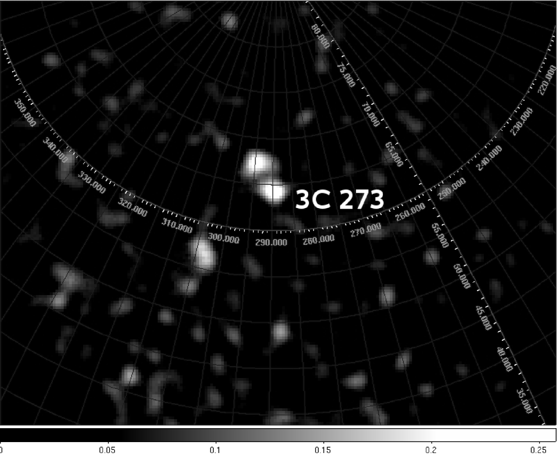
Figure 2: Sky Image of Virgo region in gamma-rays obtained from GRID instrument onboard AGILE, from 2007-12-24 07:11:47 to 2007-12-30 23:03:06 UT, for E $>$ 100 MeV. The angular dimensions of the image is 60^∘ width by 45^∘ height. The spot up/left near 3C 273 is the unidentified source, while the dimmer spot down/left is 3C 279.

The sky image in the energy range 100 MeV - 50 GeV, exposed for the 7 central days of the observation, is shown in figure 2. The unidentified source is clearly visible in the image. 3C 279, the other well known blazar in the Virgo Region, appears very faint, with a significance of 2.9 as measured by the $T_{S}$ parameter (Mattox et al (1996)).

We found that by selecting the energy range 100 - 200 MeV we could obtain a good rejection of the photons from the unidentified source, still keeping the signal-to-noise ratio for 3C 273 unaffected. This suggests that the unidentified source has a very hard energy spectrum.

In the first and third week of our campaign 3C 273 was not detected by the GRID, while in the second week it was detected at a rather high gamma-ray activity, with a flux comparable to the EGRET detection of the June 1991. The results of the analysis of the GRID data is reported in table 2 for the three individual blocks and for the whole period, both for the 100-200 MeV and $>$100 MeV energy bands. Upper limits with 95% confidence level are provided for the first and third week, when our analysis provided flux estimations with $\sqrt{T_{S}}\ <$ 3 (Mattox et al (1996)). The same data are also shown in the top panel of fig. 1. As mentioned above, in the third observing block the exposure lasted 4 days only, and the unidentified source was very bright, thus the corresponding upper limits are higher with respect to the first observing block.

Table 2: 3C 273 Flux measurements from the GRID instrument. For the first and third block/week the $\sqrt{T_{S}}$ column provides the value obtained by the standard processing.

energy	Flux during	$\sqrt{T_{S}}$	Flux during	$\sqrt{T_{S}}$	Flux during	$\sqrt{T_{S}}$	Flux during	$\sqrt{T_{S}}$
range	observing block 1		observing block 2		observing block 3		observing block 1+2+3
(MeV)	$(10^{-8}\ \gamma/cm^{2}/s)$		$(10^{-8}\ \gamma/cm^{2}/s)$		$(10^{-8}\ \gamma/cm^{2}/s)$		$(10^{-8}\ \gamma/cm^{2}/s)$
$100\div 200$	$<15$	0.2	$34_{-10}^{+12}$	4.6	$<37$	0.9	$17\pm 6$	3.8
$>100$	$<20$	1.4	$33\pm 11$	4.4	$<50$	1.5	$22\pm 6$	4.6

3.2 SuperAGILE data

The AGILE/SuperAGILE instrument (Feroci et al. (2007)) provided images of 3C 273 in the energy range 18-60 keV, during the same period of the GRID. Based on the available statistics, we divided the complete 3-week observation in 5 bins of 3-4 days each. The first two SA bins are simultaneous to the first GRID block, the next two bins are simultaneous to the second GRID block, while the last SA bin is simultaneous to the third GRID block, due to the shorter exposure in the third week.

The SA instrument is a one-dimensional coded-mask imager, producing two orthogonal one-dimensional sky images of the observed sky, starting from photon-by-photon data on user-defined time intervals. As an example, the sky image provided for one of the two instrumental coordinate (the X coding direction) accumulated over the third and fourth time-bins is shown in fig. 3.

Figure 3: One-dimensional sky image of Virgo field in hard X obtained from SuperAGILE instrument onboard AGILE, where only 3C 273 shows up as a peak. Data were integrated from 2007-12-24 07:11:47 to 2007-12-30 23:03:06 UT in the 20-60 keV energy range. Abscissa reports the angular distance (degrees) from the on-axis direction.

The SA data analysis was performed with the TDS source package of the SASOA pipeline (build 3.8.0). The photon lists are filtered, excluding those events taken during the satellite passage through the south Atlantic anomaly, and for events taken when the source was occulted by the Earth.

The continuous slew of the pointing direction of 1 degree/day due to the AGILE solar panel constraints, requires that the detector images accumulated from the event list are corrected using pointing information from the star-tracker data.
Dealing with a coded-mask imager, the attitude-correction depends on the source position in the field of view of each detector. Anyway, the correction to apply changes slowly with the source position in the FOV. Thence the correction calculated for a specific position $\big{[}\theta^{*}_{cod},\theta^{*}_{uncod}\big{]}$ in the FOV (where $\theta^{*}_{cod}$ and $\theta^{*}_{uncod}$ represent the positions in the coded and uncoded direction respectively) can be applied without affecting the point spread function of sources located at some degree from $\big{[}\theta^{*}_{cod},\theta^{*}_{uncod}\big{]}$. On account of this, we calculate the correction in a grid of 19x17 positions in the FOV, with a grid step of 6^∘ along the detector coded direction, and 4^∘ along the non-coded direction. Thence $19\times 17$ virtual detector images are generated from the photon list of each detector. A detailed description of the attitude correction procedure for SuperAGILE will be presented in a forthcoming paper (Pacciani et al. 2009, in preparation). A cross-correlation procedure of these detector images with the mask code provides the images of the point like sources, as shown in fig. 3.

The count rate of photons collected from each silicon $\mu$strip of the detectors is affected by the non-uniformities between the energy thresholds of the analog chains (see Pacciani et al. (2008)), and to the temperature dependance of the discriminator units. we account for this non-uniformity applyng a detector efficiency vector in the imaging procedures. The efficiency is generated from a blank field and corrected for the temperature effects. The non-uniformities in the low-energy thresholds makes it unsafe to use the 18-20 keV energy bin for long integrations, when threshold variations can critically affect the results. For our analysis we then used SA data in the 20-60 keV energy range.

The SA response was calibrated in-flight with a raster scan with the Crab Nebula, at several positions in the FOV. During our observation 3C273 scanned the central part of the FOV, ranging from 7.7 to -2.4 deg in the X instrumental coordinate and from 11.0 to -12.4 deg in the Z instrumental coordinate. Observed count rates are then converted into physical units of mCrab, by using the Crab response at the relevant position in the FOV (implicitly assuming a Crab-like energy spectrum). The average 20-60 keV flux measured by SA over the complete 3-week observation is (23.9 $\pm$ 1.2) mCrab, with a source detection significance of 14 $\sigma$ and 16 $\sigma$ in the X and Z coordinate, respectively and a net exposure to the source of 742 ks. The results of a time-resolved analysis are reported in the relevant panel of fig. 1 in the 20-60 keV energy range, adding up the normalized count rates from each one-dimensional sky image. The corresponding data are reported in the appendix, table LABEL:tab:hardx_lc_app.

3.3 INTEGRAL JEM-X, ISGRI and SPI data

Wide-band data for the source were obtained using the high-energy instruments onboard INTEGRAL, JEM-X in the effective energy range 5-20 keV, ISGRI in 18-200 keV and SPI in 100-500 keV. The effective energy ranges we used exclude the energy regions with too low effective area and the lowest energies, affected by electronic noise. For SPI we reported the energy range where the effective area is comparable or higher than the ISGRI. Data were processed using the Off-line Scientific Analysis OSA 7.0 software released by the Integral Scientific Data Centre. ISGRI light curves and spectra were extracted for each individual SCW. The spectrum from JEM-X was extracted from a mosaic image at the position of the source. Due to the dithering pointing strategy, the source is not always in the JEM-X field of view. The SPI data were integrated for the three INTEGRAL revolutions together to achieve the needed sensitivity up to 500 keV. The net exposure to the source was 122 ks for JEM-X, 580 ks for ISGRI and 494 ks for SPI. The average measured flux for each instrument was: (13.81$\pm$0.25) mCrab in 5-20 keV (JEM-X, 56 $\sigma$ detection significance), (22.30$\pm$0.32) mCrab in 20-60 keV (ISGRI, 70 $\sigma$ detection significance), and (41$\pm$9) mCrab in 100-500 keV (SPI, 4.4 $\sigma$ detection significance) which provides a marginal detection.
The light curves in the energy ranges 5-20, 20-60, 60-100, 100-200 keV from the above instruments are shown in figure 1 with a bin size of 200 ks (an INTEGRAL revolution), except for the 20-60 keV energy range, where the counting statistics allowed for a 25 ks bin size. The data are reported in table LABEL:tab:hardx_lc_app of the appendix. The simultaneous 20-60 keV flux measurements by SuperAGILE and ISGRI appear in good agreement.

The spectra taken during the three individual INTEGRAL revolutions, can be fitted with a simple power law model in the 18-120 keV energy range. The best-fit parameters are reported in table 3. No significant spectral evolution is detected, except for a marginal evidence of softening in the spectrum from revolution 635.

Table 3: Spectral fitting parameters in the 18-120 keV energy range (uncertainties at 90% level).

	$1^{st}$ week	$2^{Nd}$ week	$3^{rd}$ week
	(rev 633)	(rev 635)	(rev 637)
photon index	$1.77\pm 0.07$	$1.87\pm 0.09$	$1.80\pm 0.07$
flux (20-40 keV)	$173\pm 5$	$144\pm 5$	$169\pm 5$
10-12 erg cm${}^{-2}\ s^{-1}$

3.4 Hard X-ray data from BAT

Flux measurements of the sources serendipitously observed by the BAT instrument onboard Swift are available on-line for every satellite orbit. The flux measurements are sparse and with different exposure, depending on the specific satellite pointing strategy. We grouped the available data with bin size of 3 days. To account for the huge spread in the signal to noise ratio between data, a weighting factor inversely proportional to the flux error was applied during the rebinning operation.

The BAT light curve in the range $15\ -\ 50$ keV is shown in figure 1 and reported in table LABEL:tab:hardx_lc_app of the appendix. The light curve from BAT has the same trend as the SuperAGILE and ISGRI instruments but a slightly lower flux, likely due to the slightly different bandpass.

3.5 XRT data

For the analysis of soft X-ray data from the Swift X-Ray Telescope (XRT), we used the version 11.6 of the XRT pipeline. Grade filtering was applied by selecting the 0-2 and 0-12 ranges for the data collected in WT and PC mode, respectively. The data collected in PC mode are affected by pile-up in both observational epochs (average count rate $\sim$8 counts/s). The pile-up estimation and correction was made more difficult by the presence of a bad column crossing the center of the source extraction region in both observational epochs. Thus, we could obtain only a rough estimation of the pile-up effects and decided to use only the data collected in Windowed Timing mode, not affected by pile-up.

To account for the bad column in the light curve and spectra extraction, we used the exposure maps computed for each epoch and from them we generated the ancillary response files. The latter are very sensitive to the source centroid position on the CCD. But due to the bad column, we could not evaluate the centroid accurately and therefore run the pipeline fixing the source position at the coordinates given from optical and radio observations in the SIMBAD archive. The Swift star sensors precision introduces a systematic uncertainty in the evaluation of the satellite pointing, providing a mismatch between the source centroid on the CCD evaluated with the star sensors data and the effective one. In order to evaluate the effects of this systematics on the flux and spectral index estimation, we computed the effective area also over two other positions shifted of 3.1” (a region that encloses 90% of the Point Spread Function from the SIMBAD one).
The signal was extracted from a rectangular region (40 pixels wide and 20 pixels in height), assuming as nominal the position centered on the SIMBAD coordinates. The difference between the results obtained at the SIMBAD position and the shifted ones is then taken as a systematic uncertainty, denoted below as ”(syst)”. Assuming an absorbed simple power law spectral model, with absorption fixed at $N_{H}=1.79\times 10^{20}$ cm^-2 (Kalberla et al. 2005), we found a photon index of $1.61\pm 0.05$, with an observed 2-10 keV flux of $1.85\times 10^{-10}\ \pm\ 0.04\ (stat)\ \pm 0.03\ (syst)$ erg cm^-2 s^-1 during the first epoch (reduced $\chi^{2}$ is 0.9, 92 d.o.f.). No significant variations were observed during the second epoch, where the photon index is $1.57\pm 0.06$ and the observed 2-10 keV flux is $1.75\times 10^{-10}\ \pm\ 0.04\ (stat)\ \pm 0.08\ (syst)$ erg cm^-2 s^-1 (reduced $\chi^{2}$ is 1.0, 71 d.o.f.). The bad quality of the image in the second observation caused the systematics to be higher. The star sensor systematics does not affect the photon index estimation in WT mode.
XRT data are shown in figure 1.

3.6 UVOT data

UV data reduction and photometry of the source was performed using the standard UVOT software developed and distributed within the HEAsoft 6.3.2 by the NASA/HEASARC and the most recent calibrations included in the last release (2007-07-11) of the “Calibration Database” (CALDB; see also Poole (2008)). Source counts were extracted for all filters from circular aperture of 5″  radius, the background from source-free circular aperture of 12″ radius and count-rates converted to fluxes using the standard zero points. The count-rate of the source is near the limit of acceptability for the “coincidence loss” correction factor included in the CALDB ($\sim$ 90 cts s^-1), in filters U, B, UVW1 and UVW2 for both observations. We considered in our analysis only the V and UVM2 filters for both the observations and also the B for the second. The fluxes were then de-reddened using a value for $E(B-V)$ of 0.021 mag (Schlegel et al. (1998)) with $A_{\lambda}/E(B-V)$ ratios calculated for UVOT filters (for the latest effective wavelengths) using the mean Galactic interstellar extinction curve from Fitzpatrick (1999). No significant variability was detected within each single exposure for both the observations.
UVOT data are shown in figure 1 and reported in table LABEL:tabapp:rem_lc_app of the appendix.

3.7 REM data

Data reduction and photometry of the near-IR and optical frames from the REM observations has been carried out through the GAIA software using images corrected by bias, dark and flat-field (see Stetson (1987)). The instrumental magnitudes have been calibrated using the comparison star sequences reported in Gonzales et al. (2001) for the optical and the near-IR bands. Three bright isolated stars in the field of view were used as reference to calculate the instrumental magnitude shift.
The near infrared and optical light curves over a 34 days monitoring for the K, H, J, I, R, V bands of REM observatory are shown in figure 1 and reported in table LABEL:tabapp:rem_lc_app of the appendix. The large errors for some data point are due to the presence of the moon, causing errors in the photometry of 3C 273 and/or of the reference stars. Small differences in the simultaneous measurements in the UVOT/V and REM/V bands are most likely to be ascribed to the slightly different bandpass, as reported in table LABEL:tabapp:rem_lc_app.

4 Discussion

From the multi-frequency light curves shown in fig. 1, the source exhibited gamma-ray activity in the second week of the AGILE observation. In the same time period, a $\sim 20\%$ reduction in the X- and hard X-ray flux was detected by all the involved instruments. Instead, the near-IR, optical and UV fluxes remained constant to within $\sim 10\%$ variability. No strong evidence for correlations can then be derived between the gamma-ray activity and the source emission in other bands, using the analysis of the light curves.

In order to study the spectral variability, in the following we divided the campaign in 3-weeks, according to the GRID observing blocks. We first evaluated the possible contribution of a Seyfert-like reflection component in the X-ray/soft gamma-ray energy spectrum, and then build the complete Spectral Energy Distribution for two epochs, to understand the origin of the gamma-ray activity.

4.1 Limits on Seyfert-like spectral features

The wide band energy spectra of the source taken by BeppoSAX between 1997 and 2000 allowed to disentangle the contribution of the jet and Seyfert-like features (see Grandi and Palumbo (2004)). The XRT calibration status below 0.6 keV (see Cusumano (2007)) does not allow us to study the soft excess, while the Iron line studies (Yaqoob and Serlemitsos (2000) and references therein) are prevented to us by the counting statistics. Instead, our data allow us to study the reflection hump contribution to the spectra, emerging at 20-60 keV.

Unfortunately, results in this spectral region are very sensitive to possible uncertainties in the cross-calibrations between JEM-X and ISGRI instruments. In the $3^{rd}$ IACHEC meeting (held in Schloss Ringberg, Germany May 18-21 2008), cross-calibration factors near to unity were reported for the instruments onboard INTEGRAL (see the J. P. Roques presentation) for the Crab observations. In the following we use that cross calibration factors for the instruments onboard INTEGRAL, and keep free the XRT normalization factor (also to account for the systematics in XRT data relative to our specific observation). It is also important to note here that the declared INTEGRAL cross-calibration factors are reported for Crab-like spectra, while the energy spectrum of 3C 273 is harder (table 3). In order to account for possible spectral dependence of the cross-calibration constants, we always kept the JEM-X factor fixed (to 1.02) and fixed the ISGRI constant to 3 possible values, reporting the best-fit results in all the three cases. SPI data were not used in this analysis.

We built three energy spectra (one per INTEGRAL revolution). Each spectrum contains the ISGRI data for that revolution. The first XRT observation was performed 1.5 days after the end of the last INTEGRAL pointing, thence we used XRT data for the third spectrum only. In order to reach enough significance, all the JEM-X data of the campaign were merged together in the spectrum of the third week. We corrected the JEM-X multiplicative factor to account for the true normalization factor for the third week (during the third week the JEM-X flux was 1.08 times the mean flux of the campaign).

The energy spectra of the three epochs were fitted simultaneously. We first attempted a fit with an absorbed simple power law plus a Compton reflection hump described by the PEXRAV model in the XSPEC package (Magdziarz & Zdziarski (1995)). We used the PEXRAV parameters set proposed in Grandi and Palumbo (2004), with only the PEXRAV normalization allowed to vary in the fitting, but linked for the three epochs. The photoelectric absorption column was fixed to the Galactic value of $N_{H}\ =\ 1.79\cdot 10^{20}$ cm^-2 (Dickey and Lockman (1995)). The power law parameters were linked for the three epochs, except for their normalization, left completely free to vary. With this approach, we tested the hypothesis that the hard X-ray variability among the three epochs was entirely due to the jet-component. The best-fit result is marginally acceptable ($\chi^{2}/d.o.f.$=1.15, 47 d.o.f., null hypothesis probability 0.24).

We then introduced a break in the description of the jet component (that is, we introduced a broken power law in place of the simple power law) and adopted the same fitting strategy, again under the hypothesis of a variability entirely due to the jet component. An acceptable fit was achieved, and the best fit results are reported in the first column of table 4, where uncertainties on parameters are computed at 90% for one interesting parameter. We note that using only a broken power law without a reflection component provides a significantly worse best-fit result, with a $\chi^{2}/d.o.f.$ of 1.20 (46 d.o.f., null hypothesis probability 0.17). Interestingly, the fit would become fully acceptable if the JEM-X/ISGRI cross-calibration is allowed to go in the range $C_{ISGRI}/C_{JEM-X}=1.25\div 1.30$.

To the aim of providing the reader with the confidence on how strong the need for a Compton reflection component is in our spectra, we also studied the case where the difference in spectrum between Crab and 3C 273 may bring to a different cross-calibration factor between JEM-X and ISGRI. We tested the cases of $C_{ISGRI}=0.89$ and $C_{ISGRI}=1.09$, and the best-fit parameters are given in columns 2 and 3 of table 4. As expected from our previous discussion, the higher the ISGRI/JEM-X cross-calibration factor is, the lower is the needed contribution by the Compton reflection. But a minimum value of 1.25 is needed to exclude it, and this contrasts with the latest releases by the hardware teams.

We note that the uncertainties on the normalization factor for the PEXRAV and broken power law (indicated respectively as $N_{Pex}$ and $N_{Bkp}$ in table 4) are correlated. Therefore, in order to compare the contribution of the jet in the three epochs, here in terms of the value of the normalization of the broken power law, we performed another fit by fixing the PEXRAV parameters to their best fit value. The uncertainty on the $N_{Bkp}$ under this assumption are provided in parenthesis in column 1 of table 4, showing that the jet-component variation between the first and the second week is indeed statistically significant, while the difference between the values in the second and third is marginally consistent with the combined 90% uncertainties on the individual parameters. The spectral energy densities for each week with the best-fit models are shown in fig. 4. The reflection hump discussed in the previous section is not included in the model.

Thus, from our analysis of the time-resolved X-to-soft-gamma-ray energy spectrum, we can derive that the variability observed from the light curves in this energy range is most likely due to the jet component, described as a broken power law in our emission model, although a non-variable reflection component is also required by the spectral data presented here.

Table 4: Best-fit results for the simultaneous spectral fit of the three epochs (see text for details). We report the values obtained for the nominal Crab cross-calibration factor of ISGRI ($C_{ISGRI}=0.99$), and for $C_{ISGRI}=0.89$ and $C_{ISGRI}=1.09$. $N_{Pex}$ and $N_{Bkp}$ are the normalization factors for the PEXRAV and broken power law models respectively (reported as photon flux at 1 keV in units of $10^{-3}\ ph/cm^{2}/s/keV$). $\ \ \ {}^{*}$ error obtained fixing the PEXRAV normalization.

	$C_{ISGRI}=0.99$	$C_{ISGRI}=0.89$	$C_{ISGRI}=1.09$
	(nominal from Crab)
$N_{Pex}$ ($10^{-3}\ ph/cm^{2}/s/keV$)	$13.3\pm 5.0$ ($\pm 0$)∗	$19.4\pm 5.3$	$7.9\pm 4.7$
$N_{Bkp}$ for rev. 633 ($10^{-3}\ ph/cm^{2}/s/keV$)	$27.1\pm 9.3$ ($\pm 5.1$)∗	$20.3\pm 9.5$	$33.8\pm 9.3$
$N_{Bkp}$ for rev. 635 ($10^{-3}\ ph/cm^{2}/s/keV$)	$19.5\pm 7.9$ ($\pm 3.8$)∗	$13.5\pm 7.8$	$25.7\pm 8.0$
$N_{Bkp}$ for rev. 637 ($10^{-3}\ ph/cm^{2}/s/keV$)	$25.4\pm 8.6$ ($\pm 4.7$)∗	$18.7\pm 8.7$	$32.0\pm 8.6$
photon index 1	$1.46\pm 0.12$ ($\pm 0.10$)∗	$1.38\pm 0.15$	$1.51\pm 0.10$
photon index 2	$1.71\pm 0.05$ ($\pm 0.04$)∗	$1.66\pm 0.05$	$1.75\pm 0.04$
break Energy (keV)	$4.\pm 2.$ ($\pm 2.$)∗	$4.\pm 2.$	$4.\pm 2.$
XRT cross-calib	$1.01\pm 0.11$ ($\pm 0.11$)∗	$1.02\pm 0.11$	$0.98\pm 0.11$
$\chi^{2}/d.o.f.$	38.0/45	40.7/45	36.4/45
null hypothesis probability	0.76	0.65	0.82

Figure 4: Hard X spectral energy density obtained with ISGRI data for the 3-weeks of the campaign. Each column refers to a week. The SED of the third week includes the JEM-X and XRT data. The overplotted curves refer to the Compton reflection hump (the lower curve), the broken power law (the middle one), and the summation of the two (upper curve). We used the INTEGRAL Cross calibrations factors obtained for the Crab.

4.2 Spectral Energy Distribution

With the aim of understanding the origin of the gamma-ray emission, we used our multi-frequency data to build a Spectral Energy Distribution (SED). Due to the uncertainty in the evaluation of the gamma-ray flux of 3C 273 for the third week, in the following we refer mainly to the first and the second week of observations.

We made the following approximations in the evaluation of the SED. Similarly to the case discussed in the previous section, for JEM-X we used the spectrum extracted from all the three JEM-X observations together, and we applied a correction factor to the spectra to obtain the observed count rate (in the 5-20 keV band) from each revolution. Due to the statistics, the SPI data are obtained from the integration of the three INTEGRAL revolutions together. Finally, we assumed a photon index of 2.4 to convert counts to photons in the AGILE GRID data.

The resulting SEDs for the first and second week are shown in fig. 5. We described the broad band emission in the framework of a model including synchrotron emission, synchrotron self Compton and external Compton components (see Maraschi, Ghisellini, Celotti (1992), Marsher & Bloom (1992), Sikora et al. (1994)). We didn’t take into account the reflection hump in the SED model.
Remarkably, the flux distribution in our high gamma-ray state period is similar to that measured during the multi-wavelength campaign performed in June 1991, when gamma-ray variability was not observed. In that campaign (Lichti et al (1995)) the gamma-ray flux was $(56\ \pm\ 8)\cdot 10^{-8}$ photon $cm^{-2}s^{-1}$ for E $>$ 70 MeV, and the photon index $2.39\ \pm 0.13$, consistent with the AGILE flux of $\big{(}34_{-10}^{+12}\big{)}\cdot 10^{-8}$ $\ photon\ cm^{-2}s^{-1}$ for E $>$ 100 MeV.

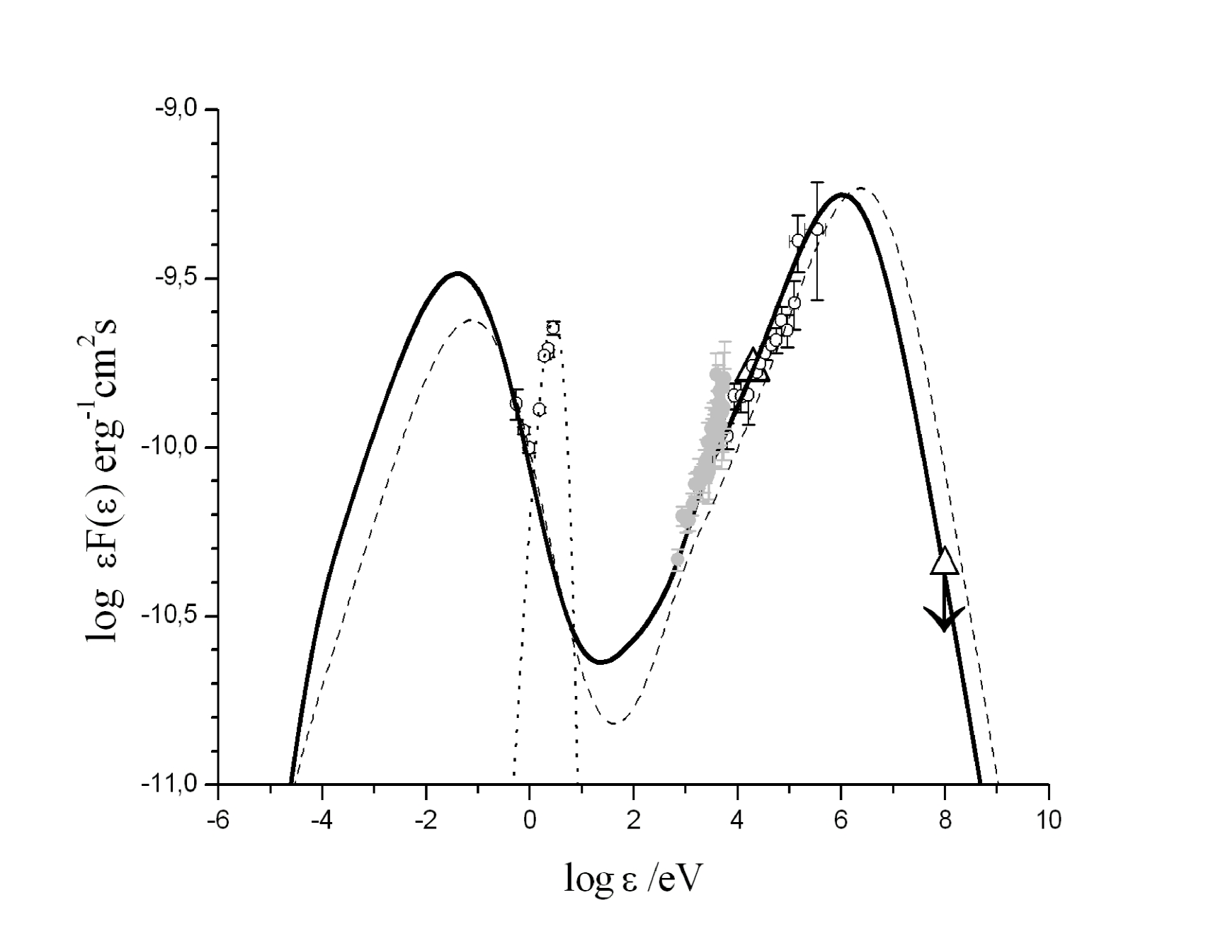
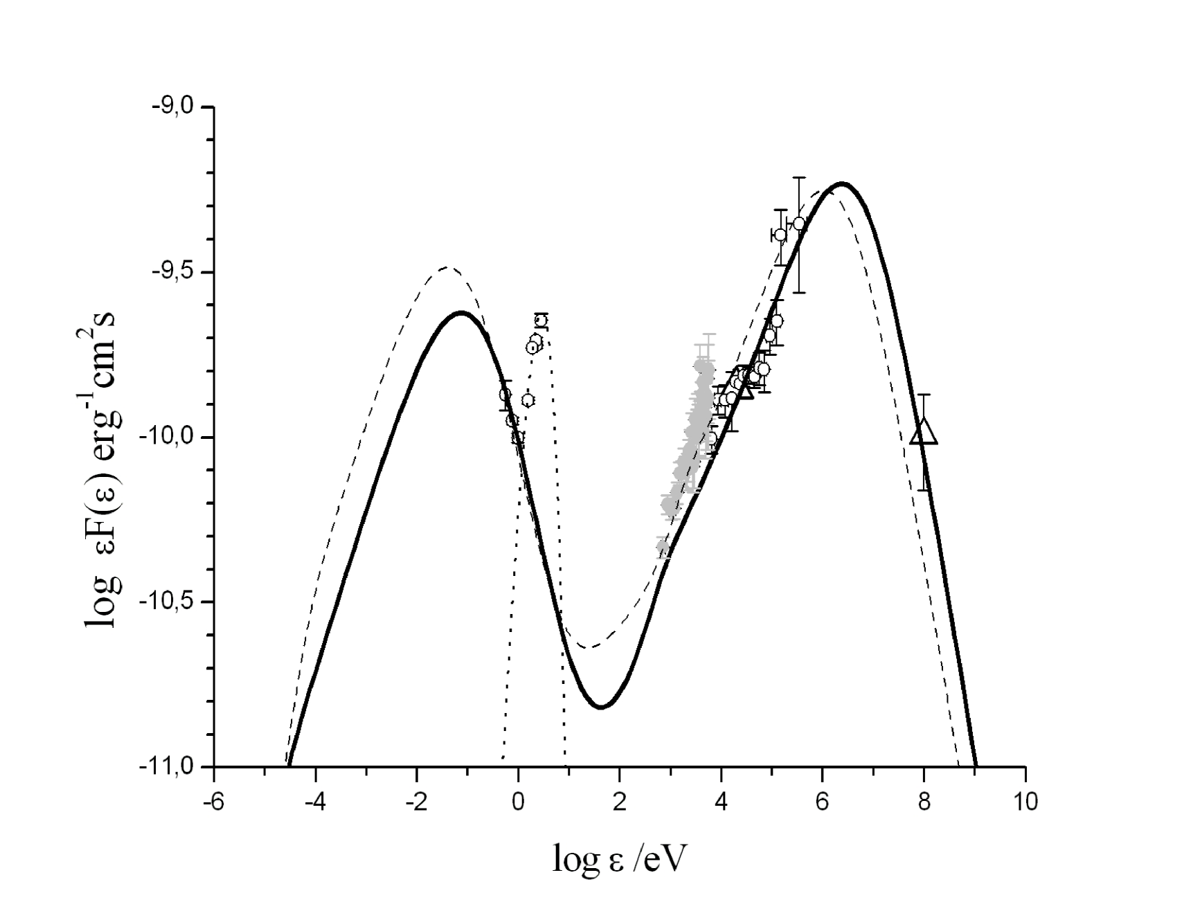
Figure 5: Spectral Energy Distribution of 3C 273 for the first (top panel) and the second week (bottom panel). Triangles are for AGILE data. The grey data refers to the XRT observations, performed in the third week. The line is the model for the simultaneous data of the week. The model for the other week is reported for comparison as dashed line. The reflection hump is not included in the model. Where not visible the energy range is smaller than the symbol.

The observed variability of the SED between the two epochs cannot be associated to a synchrotron flare. In that case an enhancement of the emission at all the observed wavelengths is expected. The variability behaviour can be reproduced as a shift toward higher energies of the electron density, thence related not to the injection of a new blob, but to electron acceleration. According to this hypothesis, we modelled the variability keeping the bulk Doppler factor, the blob radius and the disk luminosity unchanged. Instead, we varied the parameters related to the accelerated electrons: i.e. the electrons energy distribution ($n_{e}$, $\gamma^{*}$ and $p_{2}$) and, slightly, the tangled magnetic field. But the choice of the SED parameters allowing for a change from the first to the second week is not unique. The chosen parameters of the SED model for the two epochs are reported in table 5.

Actually, the spectral variability that we observed can be interpreted in the context of standard model of FSRQ as follows. The flux at frequencies $>3\cdot 10^{14}$ Hz, consistently with the large ($6^{\circ}$) viewing angle, appears dominated by thermal emission from the disk and/or from the BLR. Thus, we expect the emission in the range of frequencies observed by REM to not vary on daily timescales, and to hide variations of the synchrotron emission except in the near-IR (K and H bands). The REM observations, show variations lower than $\sim 10-15\%$ in the near-IR and optical. Our model, showed in fig. 5, produce no variations of the synchrotron emission in the near-IR and optical energy regions.
A moderate shift of the direct synchrotron spectrum towards higher frequencies is detectable in the far-IR and in the soft X (if not hidden by other thermal components, e.g. the components suggested in Turler et al. (2006), and the soft excess reported in Grandi and Palumbo (2004)). But we didn’t have coverage of that energy regions for all the campaign.

Variations are instead revealed in the inverse Compton reprocessing in the X-ray and gamma-ray domain. The relative variations that we detected, $\sim$20-30$\%$ and a factor $\sim$2-3, respectively, together with the fact that the gamma-ray flux appears anti-correlated to the X-ray flux, indicates that a shift toward higher energy in the electron density is very likely responsible for the observed variability.

In the model, the associated SSC variation reflects in a moderate decrease of the leading edge of the SED in the soft X-ray band, whereas the EC by the disk shows up as a flux decrease in the hard X-rays. In the gamma-ray band, the falling portion of the EC spectral energy distribution well describes the observed enhancement.

Table 5: Parameters for the spectral energy distribution for the first and second week of the campaign. $p_{1}$ and $p_{2}$ are the pre and post break spectral index for the electron population, $\gamma^{*}$ is the break energy Lorentz factor, $\gamma_{min}$ is the cut-off energy of the electron population, B the tangled magnetic field, $r$ the radius of the spherical blob in the comoving frame, $\delta$ the Doppler factor, $n_{e}$ the electron density.

week	$p_{1}$	$p_{2}$	$\gamma^{*}$	$\gamma_{min}$	B	r	$\delta$	disk Luminosity	$n_{e}$
					(Gauss)	($10^{16}$ cm)		($10^{45}erg\ cm^{-2}\ s^{-1}$)	($e^{-}/cm^{3}$)
first	2	5	200	3	12	2	9	6	$150$
second	2	4.7	300	3	10	2	9	6	$\ 70$

In the scenario proposed by Sikora et al. (2001), during the acceleration phase, the accelerated electrons population increases, saturating at high energy first. When the phase of electrons acceleration stops, the energy break $\gamma^{*}$ of the electrons population moves to lower energies, reaching the critical energy $\gamma_{C}$ (balancing the radiative cooling time with the duration of the acceleration period) or even lower values. In that model, the gamma-ray light curve reaches its maximum before the hard X, then decay faster than hard X-ray light curve. That scenario might be able to fit the data of our multiwavelength campaign, provided that the second week is related to an electrons acceleration phase, and the first week to the late phase of a previous episode. Thence the gamma-ray activity and the high value of $\gamma^{*}$, during the second week of observation are the signature of the acceleration phase.

5 Summary and Conclusions

We presented data of a pre-scheduled 3-week multi-wavelength campaign on 3C 273 carried out between mid-December 2007 and January 2008, covering from the near-Infrared to the gamma-ray energy bands, for the first time after the demise of the EGRET instrument. The source was found in high state in the X-rays, with a 5-100 keV flux a factor of $\sim$3 higher than the typical value in historical observations (e.g., Courvoisier et al (2003) for the INTEGRAL data). Instead, the AGILE gamma-ray data showed a flux lower-equal to the EGRET measurements, and the optical/IR measurements provided fluxes very similar to the ”standard values” for this source.

Our multi-frequency and continuous set of data allowed us to study the short-term variability (days to week) of this source. The simultaneous light curves from the different instruments do not show any strong correlation, except for an indication of an anti-correlated variability between X-rays and gamma-rays: all the soft and hard X-ray measurements show a decreasing trend at the time of our single positive detection in the gamma-rays in the second week of observation, preceded and followed by non-detections in the first and third week of our campaign.

This behavior can be interpreted and understood when we use our multi-frequency data to model the source spectral energy distribution. Using a model composed by a one-zone homogeneous Synchrotron-Self-Compton plus external Compton from an accretion disk, we find that the spectral variability between the first and the second week is consistent with an acceleration episode of the electron population responsible for the synchrotron emission. In our model the detectable synchrotron variations are in the far-IR and in the soft X-rays, where we didn’t have adequate coverage, whereas the near-IR and optical remain almost unchanged. But the signature of the acceleration is brought up by the inverse Compton peak in the X and gamma-ray energy ranges.

We note that shifts of the inverse-Compton peak from observation to observation were previously proposed (see McNaron-Brown et al (1994)) from the comparison of the June 1991 multi-wavelength campaign, and the OSSE observation of September 1994. Our multi-frequency observation and modelling suggests that this behaviour is a more general feature of this source, happening on shorter timescales.

Our observation of a weaker X-ray flux in the second week motivated us to study the Seyfert-like disk reflection hump in this source. The wide band spectral data from the INTEGRAL instruments show that the jet (non-thermal) emission alone does not describe the energy spectrum adequately. A reflection hump improves the X-ray spectral modelling. We then found that in the second week the jet contribution to the X-ray emission gets dimmer, due to the shift to higher energy of the electron population discussed above, making the likely constant disk contribution to emerge. The quality of our data did not allow to put any constraints on the possible variability of the reflection component, that in our data is consistent with an intermediate intensity reported form previous observations (e.g., Grandi and Palumbo (2004))

Appendix A Complementary data

Table 6: Hard X data from SuperAGILE and ISGRI. The Flux is reported in mCrab units in the energy band 20 - 60 keV

start date	stop date	exposure	flux	observatory
(MJD)	(MJD)	(ks)	(mCrab)
54450.72	54453.91	136	30.2 $\pm$ 2.9	SuperAGILE
54453.91	54457.10	141	24.5 $\pm$ 3.0	SuperAGILE
54458.30	54461.63	140	21.6 $\pm$ 2.2	SuperAGILE
54461.63	54464.96	150	21.2 $\pm$ 2.4	SuperAGILE
54469.57	54473.46	176	22.2 $\pm$ 2.3	SuperAGILE
54453.86	54454.14	21	25.7 $\pm$ 1.6	ISGRI
54454.14	54454.43	18	22.4 $\pm$ 1.6	ISGRI
54454.43	54454.72	21	24.2 $\pm$ 2.4	ISGRI
54454.72	54455.01	22	22.4 $\pm$ 1.5	ISGRI
54455.01	54455.30	22	23.1 $\pm$ 1.5	ISGRI
54455.30	54455.59	24	23.8 $\pm$ 1.4	ISGRI
54455.59	54455.88	22	25.1 $\pm$ 1.5	ISGRI
54455.88	54456.17	22	24.0 $\pm$ 1.5	ISGRI
54456.17	54456.38	14	26.0 $\pm$ 2.9	ISGRI
54459.73	54459.93	8	18.3 $\pm$ 2.6	ISGRI
54459.93	54460.22	24	21.1 $\pm$ 1.5	ISGRI
54460.22	54460.51	23	19.3 $\pm$ 1.6	ISGRI
54460.51	54460.80	24	18.2 $\pm$ 1.5	ISGRI
54460.80	54461.09	20	17.9 $\pm$ 1.6	ISGRI
54461.09	54461.38	23	20.1 $\pm$ 1.6	ISGRI
54461.38	54461.67	24	22.2 $\pm$ 1.5	ISGRI
54461.67	54461.96	15	20.3 $\pm$ 1.9	ISGRI
54461.96	54462.25	24	20.2 $\pm$ 1.5	ISGRI
54462.25	54462.27	6	17.6 $\pm$ 4.1	ISGRI
54465.72	54466.01	16	23.2 $\pm$ 1.9	ISGRI
54466.01	54466.30	24	20.4 $\pm$ 1.4	ISGRI
54466.30	54466.59	23	19.1 $\pm$ 1.5	ISGRI
54466.59	54466.88	24	24.9 $\pm$ 1.5	ISGRI
54466.88	54467.17	23	21.7 $\pm$ 1.5	ISGRI
54467.17	54467.45	24	27.1 $\pm$ 1.5	ISGRI
54467.45	54467.74	24	22.6 $\pm$ 1.5	ISGRI
54467.74	54468.03	22	23.0 $\pm$ 1.5	ISGRI
54468.03	54468.18	21	26.1 $\pm$ 1.9	ISGRI

Table 6: continued.

Table 7: REM and UVOT data for the multiwavelength campaign

date	MJD	filter	$\lambda$	exposure	magn	energy flux	observatory
(aaaammdd)			($\AA$)	(s)		(mJy)
20080106	54471.5	UVM2	2231	729	11.16 $\pm$ 0.03	31.0 $\pm$ 0.9	UVOT
20080104	54469.7	UVM2	2231	610	11.17 $\pm$ 0.03	30.7 $\pm$ 0.9	UVOT
20080106	54471.5	B	4329	268	12.86 $\pm$ 0.02	33.2 $\pm$ 0.6	UVOT
20080106	54471.5	V	5402	268	12.67 $\pm$ 0.01	33.1 $\pm$ 0.3	UVOT
20080104	54469.7	V	5402	213	12.63 $\pm$ 0.01	34.4 $\pm$ 0.3	UVOT
20080114	54479.3	V	5496	300	12.64 $\pm$ 0.02	33.9 $\pm$ 0.7	REM
20080111	54476.3	V	5496	300	12.65 $\pm$ 0.02	33.7 $\pm$ 0.6	REM
20080106	54471.3	V	5496	300	12.53 $\pm$ 0.03	37.5 $\pm$ 0.9	REM
20080102	54467.4	V	5496	300	12.61 $\pm$ 0.04	35.1 $\pm$ 1.2	REM
20071227	54461.3	V	5496	300	12.70 $\pm$ 0.06	32.2 $\pm$ 1.7	REM
20071223	54457.3	V	5496	300	12.63 $\pm$ 0.06	34.4 $\pm$ 1.8	REM
20071220	54454.3	V	5496	300	12.58 $\pm$ 0.02	35.9 $\pm$ 0.7	REM
20071211	54445.3	V	5496	300	12.67 $\pm$ 0.06	33.3 $\pm$ 1.9	REM
20080114	54479.3	I	7895	300	12.04 $\pm$ 0.05	40.3 $\pm$ 1.8	REM
20080111	54476.3	I	7895	300	12.10 $\pm$ 0.05	38.1 $\pm$ 1.9	REM
20080106	54471.3	I	7895	300	12.02 $\pm$ 0.03	41.1 $\pm$ 1.0	REM
20080102	54467.4	I	7895	300	12.01 $\pm$ 0.03	41.5 $\pm$ 1.2	REM
20071227	54461.3	I	7895	300	12.14 $\pm$ 0.04	37.0 $\pm$ 1.3	REM
20071223	54457.3	I	7895	300	12.14 $\pm$ 0.03	37.0 $\pm$ 1.0	REM
20071220	54454.3	I	7895	300	12.06 $\pm$ 0.02	39.8 $\pm$ 0.8	REM
20071211	54445.4	I	7895	300	12.09 $\pm$ 0.03	38.7 $\pm$ 1.2	REM
20080114	54479.3	R	6396	300	12.48 $\pm$ 0.02	33.0 $\pm$ 0.7	REM
20080111	54476.3	R	6396	300	12.52 $\pm$ 0.01	31.8 $\pm$ 0.3	REM
20080106	54471.3	R	6396	300	12.40 $\pm$ 0.03	35.5 $\pm$ 0.8	REM
20080102	54467.4	R	6396	300	12.49 $\pm$ 0.04	32.7 $\pm$ 1.1	REM
20071227	54461.3	R	6396	300	12.55 $\pm$ 0.05	31.1 $\pm$ 1.5	REM
20071223	54457.3	R	6396	300	12.47 $\pm$ 0.06	33.3 $\pm$ 1.9	REM
20071220	54454.3	R	6396	300	12.45 $\pm$ 0.02	34.0 $\pm$ 0.7	REM
20071211	54445.4	R	6396	300	12.49 $\pm$ 0.03	32.8 $\pm$ 0.9	REM
20080114	54479.3	J	12596	30	11.53 $\pm$ 0.05	39.8 $\pm$ 1.9	REM
20080111	54476.3	J	12596	30	11.45 $\pm$ 0.06	42.8 $\pm$ 2.2	REM
20080106	54471.3	J	12596	30	11.22 $\pm$ 0.08	53.0 $\pm$ 3.7	REM
20080102	54467.4	J	12596	30	11.47 $\pm$ 0.03	42.1 $\pm$ 1.4	REM
20071230	54464.3	J	12596	30	11.47 $\pm$ 0.04	42.0 $\pm$ 1.4	REM
20071227	54461.3	J	12596	30	11.53 $\pm$ 0.03	39.9 $\pm$ 1.3	REM
20071223	54457.3	J	12596	30	11.55 $\pm$ 0.03	39.1 $\pm$ 1.2	REM
20071220	54454.3	J	12596	30	11.47 $\pm$ 0.04	41.9 $\pm$ 1.4	REM
20071211	54445.3	J	12596	30	11.42 $\pm$ 0.05	44.1 $\pm$ 2.1	REM
20080114	54479.3	H	15988	30	10.71 $\pm$ 0.04	56.6 $\pm$ 2.1	REM
20080111	54476.3	H	15988	30	10.68 $\pm$ 0.05	58.4 $\pm$ 2.4	REM
20080106	54471.3	H	15988	30	10.54 $\pm$ 0.07	66.7 $\pm$ 4.5	REM
20080102	54467.4	H	15988	30	10.65 $\pm$ 0.02	59.8 $\pm$ 1.3	REM
20071230	54464.3	H	15988	30	10.68 $\pm$ 0.02	58.5 $\pm$ 1.2	REM
20071227	54461.3	H	15988	30	10.69 $\pm$ 0.02	58.0 $\pm$ 1.3	REM
20071223	54457.3	H	15988	30	10.71 $\pm$ 0.02	56.6 $\pm$ 1.2	REM
20071220	54454.3	H	15988	30	10.65 $\pm$ 0.03	59.8 $\pm$ 1.5	REM
20071211	54445.4	H	15988	30	10.70 $\pm$ 0.04	57.5 $\pm$ 2.1	REM
20080114	54479.3	K	22190	30	9.70 $\pm$ 0.05	88.8 $\pm$ 4.2	REM
20080111	54476.3	K	22190	30	9.55 $\pm$ 0.08	102.0 $\pm$ 7.5	REM
20080102	54467.4	K	22190	30	9.65 $\pm$ 0.03	93.2 $\pm$ 2.3	REM
20071230	54464.4	K	22190	30	9.68 $\pm$ 0.03	91.0 $\pm$ 2.2	REM
20071227	54461.3	K	22190	30	9.67 $\pm$ 0.03	91.1 $\pm$ 2.3	REM
20071223	54457.3	K	22190	30	9.56 $\pm$ 0.03	101.3 $\pm$ 2.9	REM
20071220	54454.3	K	22190	30	9.58 $\pm$ 0.11	99.6 $\pm$ 10.1	REM
20071211	54445.4	K	22190	30	9.51 $\pm$ 0.05	105.9 $\pm$ 4.8	REM

Table 7: continued.

References

- Barbiellini et al. (2001) Barbiellini, G., Tavani, M., Argan, A., et al., 2001, Gamma 2001: Gamma-Ray Astrophysics, ed. S. Ritz, N. Gehrels, Chris R. Shrader, AIP Conf. Proc., 587, 754;
- Barthelmy et al. (2006) Barthelmy, S. D., Barbier, L. M., Cummings, J. R., et al., 2005, SSRv 120, 143;
- Bignami et al. (1981) Bignami, G. F., Bennett, K., Buccheri, R., et al., 1981, A&A, 93, 71;
- Boutelier et al. (2008) Boutelier, T.,Henry, G.,Petrucci, P. O., Accepted by MNRAS, and arXiv:0807.4998v1;
- Burrows et al. (2005) Burrows, D. N., Hill, J. E., Nousek, J. A., et al., 2005, SSRv, 120, 165;
- Collmar et al. (2000) Collmar, W., Reimer, O., Bennett, K., et al., 2000, A&A, 354, 513;
- Courvoisier et al (2003) Courvoisier, T. J.-L., Beckmann, V., Bourban, G., et al., 2003, A&A, 411, L343;
- Cusumano (2007) Cusumano, G., submitted to IL NUOVO CIMENTO, and arXiv:astro-ph/0701813v1;
- Dickey and Lockman (1995) Dickey, J. M., and Lockman, F. J., 1990, ARA&A, 28, 215;
- Feroci et al. (2007) Feroci, M., Costa, E., Soffitta, P., et al., 2007, Nucl. Instr. and Meth. A, 581, 728;
- Fitzpatrick (1999) Fitzpatrick, E. L., 1999, PASP 111, 63;
- Grandi and Palumbo (2004) Grandi, P., and Palumbo, G., 2004, Sci, 306, L998;
- Gonzales et al. (2001) Gonzàlez-Pèrez J. N., Kidger, M. R., and Martìn-Luis, F., 2001, AJ, 122, 2055;
- Lawson et al. (1998) Lawson, A. J., McHardy, I. M., and Newsam, A. M., 1998, Nucl. Phys. B, 69/1-3, 439-444;
- Levine et al. (1996) A. M. Levine et al, Levine, A. M., Bradt, H., Cui, W., et al., 1996, ApJ, 469, L33;
- Lichti et al (1995) Lichti, G. G., Balonek, T., Courvoisier, T. J.-L., et al., 1995, A&A 298, 711;
- Lund et al. (2003) Lund, N.; Budtz-Jorgensen, C., Westergaard, N. J., et al., 2003, A&A, 411, L231;
- Magdziarz & Zdziarski (1995) Magdziarz, P., and Zdziarski, A. A., 1995, MNRAS, 273, 837;
- Maraschi, Ghisellini, Celotti (1992) Maraschi. L., Ghisellini, G., and Celotti, A., 1992, ApJ, L5;
- Marsher & Bloom (1992) Marscher, A. P., and Bloom, S. D., 1992, Proceedings of The Compton Observatory Science Workshop, 346;
- Mattox et al (1996) Mattox, J. R., Bertsch, D. L., Chiang, J., et al., 1996, J. R. Mattox et al., ApJ, 461, 396;
- McNaron-Brown et al (1994) McNaron-Brown, K., Johnson, W. N., Dermer, C. D., and Kurfess, J. D., 1997, ApJ, 474, L85;
- Pacciani et al. (2008) Pacciani, L., Uberti, O., Del Monte, E., et al., 2008, Nucl. Instr. and Meth. A, 593, 367;
- Poole (2008) Poole, T. S., Breeveld, A. A., Page, M. J., et al., 2008, MNRAS, 383, 627;
- M. Prest et al. (2003) Prest, M., Barbiellini, G., Bordignon, G., et al., 2003, Nucl. Instr. and Meth. A, 501, 280;
- Roming et al. (2005) Roming, P. W. A, Kennedy, T. E., Mason, K. O., et al., 2005, SSRv, 120, 95;
- Schlegel et al. (1998) Schlegel, D. J., Finkbeiner, D. P., and Davis, M., 1998, ApJ, 500, 525;
- Sikora et al. (1994) Sikora, M., Begelman M. C., and Rees, M., 1994, ApJ, 421, 153;
- Sikora et al. (2001) Sikora, M., Blazejowski, M., Begelman, M. C., Modersky, R., 2001, ApJ, 554, 1; erratum: 2001, ApJ, 561, 1154;
- Stetson (1987) Stetson, P. B., 1987, PASP, 99, 191;
- Sokolov et al. (2004) Sokolov, A., Marscher, A. P., and McHardy, I. M., 2004, Apj, 613, 725;
- Swanenburg et al. (1978) Swanenburg, B. N., Hermsen, W., and Bennett, K., 1978, Nat, 275, 298;
- Tavani et al. (2008) Tavani, M., Barbiellini, G., Argan, A., et al., 2008, submitted to A&A, and arXiv:astro-ph/0807.4254v1;
- Turler et al. (2006) Turler, M., Chernyakova, M., Courvoisier, T. J.-L., et al., 2006, A&A, 451, L1;
- Ubertini et al. (2003) Ubertini, R., Lebrun, F., di Cocco, G., et al., 2003, A&A, 411, 131;
- Urry and Padovani (1995) Urry, C. M., and Padovani, P., 1995, PASP, 107, 803;
- Vedrenne et al. (2003) Vedrenne, G., Roques, J.-P., Schonfelder, V., et al., 2003, A&A, 411, 63;
- Montigny et al. (1997) von Montigny, C., Aller, H., Aller, M., et al., 1997, ApJ, 483, 161;
- Winkler et al. (2003) Winkler, C., Gehrels, N., Schonfelder, V., et al., 2003, A&A, 411, L349;
- Yaqoob and Serlemitsos (2000) Yaqoob, T., Serlemitsos, P., 2000, Apj, 544, L95;
- Zerbi et al (2001) Zerbi, R. M., Chincarini, G., Ghisellini, G., et al., 2001, AN, 322, 275;