A note on differences between (4+1)- and (5+1)-dimensional anisotropic cosmology in the presence of the Gauss-Bonnet term

Abstract

We investigate a flat anisotropic (5+1)-dimensional cosmological model in the presence of the Gauss-Bonnet (GB) contribution in addition to usual Einstein term in the action. We compared it with (4+1)-dimensional case and found a substantial difference in corresponding cosmological dynamics. This difference is manifested in the probability of the model to have smooth transition from GB-term-dominated to Einstein-term-dominated phases—this probability in a reasonable measure on the initial condition space is almost zero for (4+1) case and about 60$\%$ for (5+1) case. We discuss this difference as well as some features of the dynamics of the considered model.

The Lovelock gravity Lovelock have been intensively studied last several years (see, for example moreGB ; Maeda1 ; Maeda2.Maeda3; Ferraro ; Barrau ; Maeda4 ; Cai ; Giribet ; D1 ; D2 ; Paddy ) showing a revival of interest to this theory after about a decade of rather slow progress (for achievements of 80-th and early 90-th of the last century see, for example, evenmoreGB ; N1 ; N2 ; Kitaura ). The main feature of this extension of the General Relativity is that the resulting equations of motion are second order differential equations, in contrast to 4-th order equations in other modified gravity theories. Another important feature of Lovelock gravity is finite number of terms in the Lagrangian in contrast to string gravity, where there is an infinite row of additional terms. This means that in perturbative string gravity we can study effects arising from corrections to GR only at the level of small perturbations, otherwise it would be necessary to include all infinite set of terms into analysis. In Lovelock gravity it is possible to study regimes with non-Einstein terms being equally or more important than the Einstein part of the action.

The Lagrangian of Lovelock gravity in an $N$-dimensional space consists of all terms which are topological invariants in lower dimensional spaces. As a result, there are no corrections to Einstein theory in ($3+1$) dimensions: the second curvature invariant, Gauss-Bonnet term, appears in four dimensions and have a contribution to the equations of motion for $N>4$. The third invariant, cubic in curvature, starts to contribute from ($6+1$) dimensions etc. In the present paper we study a flat anisotropic ($5+1$)-dimensional Universe, so the Lovelock Lagrangian has only one additional term in the form of the Gauss-Bonnet combination.

In the multidimensional anisotropic cosmology the GB-term leads to two qualitatively new features. A new type of singularity with finite scale factors and energy density and diverging time derivatives appears NS ; NS2 ; NS3 , and recollaps of a flat Universe becomes possible rc . In the recent paper s_ind it was shown that in the dynamics of a ($4+1$)-dimensional anisotropic Universe these two regimes are in some sense typical, and in most cases they prevent the Universe from reaching a low-energy regime from a standard Big Bang singularity. Only special initial conditions with three equal Hubble parameters allow smooth evolution from Big Bang singularity to a 4-dimensional Kasner regime (which is exact solution in Einstein gravity), all other trajectories either describe recollapsing Universe or meet the nonstandard singularity.

In the present paper we provide a similar analysis for a flat ($5+1$)-dimensional Universe in Lovelock gravity. We show that the former result is valid only for that particular number of space-time dimensions, and though in the ($5+1$)-dimensional case there are no additional terms in Lovelock Lagrangian in comparison with the ($4+1$)-dimensional one, the smooth evolution from high-energy to low-energy regimes in ($5+1$)-dimensional Universe is typical and does not require severe fine-tuning of the initial conditions.

We consider a flat anisotropic Universe with the metrics $g_{ik}=diag(-1,a^{2},b^{2},c^{2},d^{2},e^{2})$ and the action

$$S=\int\sqrt{-g}(R+\alpha GB)d^{6}x,$$

where the Gauss-Bonnet term

$$GB=R^{iklm}R_{iklm}-4R^{ik}R_{ik}+R^{2}.$$

Introducing five Hubble parameters in a standard way, it is possible to write down equations of motion in the form of first integral

$$\begin{array}[]{l}2H_{a}H_{b}+2H_{a}H_{c}+2H_{a}H_{d}+2H_{a}H_{f}+2H_{b}H_{c}+2H_{b}H_{d}+2H_{b}H_{f}+2H_{c}H_{d}\\ \\ +2H_{c}H_{f}+2H_{d}H_{f}+24\alpha\left[\right.H_{a}H_{b}H_{c}H_{d}+H_{a}H_{b}H_{c}H_{f}+H_{a}H_{b}H_{d}H_{f}\\ \\ \left.+H_{a}H_{c}H_{d}H_{f}+H_{b}H_{c}H_{d}H_{f}\right]=0,\end{array}$$ (1)

and five dynamical equations. The first equation of motion has the form

$$\begin{array}[]{l}2(\dot{H}_{b}+H_{b}^{2})+2(\dot{H}_{c}+H_{c}^{2})+2(\dot{H}_{d}+H_{d}^{2})+2(\dot{H}_{f}+H_{f}^{2})+2H_{b}H_{c}+2H_{b}H_{d}\\ \\ +2H_{b}H_{f}+2H_{c}H_{d}+2H_{c}H_{f}+2H_{d}H_{f}++8\alpha\left[3H_{b}H_{c}H_{d}H_{f}+(\dot{H}_{b}+H_{b}^{2})\right.\\ \\ \times(H_{c}H_{d}+H_{c}H_{f}+H_{d}H_{f})+(\dot{H}_{c}+H_{c}^{2})(H_{b}H_{d}+H_{b}H_{f}+H_{d}H_{f})\\ \\ \left.+(\dot{H}_{d}+H_{d}^{2})(H_{b}H_{c}+H_{b}H_{f}+H_{c}H_{f})+(\dot{H}_{f}+H_{f}^{2})(H_{b}H_{c}+H_{b}H_{d}+H_{c}H_{d})\right]=0.\end{array}$$ (2)

four other equations can be obtained by cyclic transmutation of indices TT .

Two obvious limiting cases can be identified easily. First, in the low-curvature regime, when the contribution from the Gauss-Bonnet term is small, we have well-known generalized Kasner solution. In this solution scale factors have power-law dependence on time with the power indexes $p_{i}$, and, correspondingly, $H_{i}=p_{i}/t$ with the Kasner conditions $\sum p_{i}=1$ and $\sum p_{i}^{2}=1$.

On the other hand, when Einstein part of equations of motion are negligible in comparison with the Gauss-Bonnet contribution, another form of power-law solution exists TT . There are two form of this solution, both require $\sum\limits_{i>j>k>l}p_{i}p_{j}p_{k}p_{l}=0$, and either $\sum\limits_{i}p_{i}=3$ or $\sum\limits_{i>j>k}p_{i}p_{j}p_{k}=0$. The latter case contains solutions with $p_{i}=(a,b,0,0,0)$ where $a$ and $b$ are arbitrary numbers. In addition to discussion in TT we can show now that this form is the only possible solution of the second class up to transmutation of power indices.

Indeed, expressing $p_{1}$ from $\sum\limits_{i>j>k}p_{i}p_{j}p_{k}=0$, then substituting it into $\sum\limits_{i>j>k>l}p_{i}p_{j}p_{k}p_{l}=0$ and expressing $p_{2}$ we get

$$p_{2}=-\frac{1}{2}\frac{p_{4}p_{5}+p_{3}p_{4}+p_{3}p_{5}\pm p_{3}p_{4}p_{5}\sqrt{-3p_{4}^{2}p_{5}^{2}-2p_{3}p_{4}^{2}p_{5}-2p_{3}p_{5}^{2}p_{4}-3p_{3}^{2}p_{4}^{2}-2p_{3}^{2}p_{4}p_{5}-3p_{3}^{2}p_{5}^{2}}}{p_{3}p_{4}^{2}p_{5}+p_{3}^{2}p_{4}^{2}+p_{3}^{2}p_{4}p_{5}+p_{3}p_{5}^{2}p_{4}+p_{3}^{2}p_{5}^{2}+p_{4}^{2}p_{5}^{2}}.$$ (3)

We want to show that the expression under the radical is non-positive. To show this consider the case when this expression crosses zero:

$${\rm Det}=-(3p_{4}^{2}p_{5}^{2}+2p_{3}p_{4}^{2}p_{5}+2p_{3}p_{5}^{2}p_{4}+3p_{3}^{2}p_{4}^{2}+2p_{3}^{2}p_{4}p_{5}+3p_{3}^{2}p_{5}^{2})=0$$ (4)

It would happen when

$$p_{3}=-\frac{p_{4}p_{5}(p_{4}+p_{5}\pm 2\sqrt{-2p_{4}^{2}-p_{4}p_{5}-2p_{5}^{2}})}{3p_{4}^{2}+2p_{4}p_{5}+3p_{5}^{2}}.$$ (5)

One can easily verify that radical expression in (5) is negative for any nonzero $p_{4}$ and $p_{5}$. This means that the expression under radical in (3) has the same sign for any combination of non-zero $p_{i}$, an easy check shows that this sign is negative, ruling out all these combinations. If one of $p_{i}$ is zero, the condition $\sum\limits_{i>j>k>l}p_{i}p_{j}p_{k}p_{l}=0$ requires that at least one of remaining indexes is also equal to zero, and in this case the condition $\sum\limits_{i>j>k}p_{i}p_{j}p_{k}=0$ further requires that the third index also vanishes. As a result, the only possible form of the studied class is the combination $(a,b,0,0,0)$ found in TT .

Figure 1: Typical behavior of the model with smooth high-to-low-energy power-law regimes transition. In (a) we present the behavior of individual $H_{i}(t)$, in (b)—the expansion rate $\sum\limits_{i}H_{i}(t)$, in (c)—individual Kasner exponents $p_{i}(t)$,in (d) — the sum $\sum\limits_{i}p_{i}(t)$, and in (e) — the sum $\sum\limits_{i>j>k}p_{i}p_{j}p_{k}$.

This means that this class of solutions is a rather special one, and it is not surprising that we do not see it in our numerical simulations. From now on we consider only first class of power-law solution as a solution with standard cosmological singularity in a high-energy regime.

Apart from high-curvature and low-curvature asymptotic power-law regimes the system (1–2) describes complicated behavior in the range of Hubble parameters where both Gauss-Bonnet and Einstein contributions are important. We have studied this system numerically, starting from initial conditions distributed randomly in the interval [0,1] for three Hubble parameters, in the interval [-1,1] for one of them and calculating fifth Hubble parameter from the constraint equation (1). The integration stopped when one of the following regimes are reached:

• For expanding Universe: low-curvature Kasner regime, nonstandard singularity or recollaps.

• For contracting Universe: high-curvature power-law regime (”standard singularity”) or nonstandard singularity.

Matching two branches, expanding and contracting, of numerical solution allows us to construct a full history of the modeled Universe evolving from one of listed states to another.

The main feature which distinguishes the (5+1) case from the (4+1) one is that now the transition from a standard singularity to low-curvature Kasner regime does not require severe fine-tuning (we remind a reader that in the former case only trajectories with three scale factors equal to each other can show this type of transition).

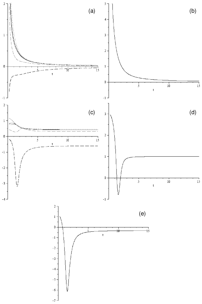
In Fig. 1 we presented a typical behavior of the model with “standard singularity” $\to$ Kasner smooth transition. In (a) panel we show $H_{i}(t)$ evolution curves, in (b) panel—$\sum\limits_{i}H_{i}(t)$; individual Kasner exponents $p_{i}$ are shown in (c) and their sum $\sum\limits_{i}p_{i}(t)$ in (d). One can easily see that this is a high-energy power-law ($\sum\limits_{i}p_{i}(t)=3$) to low-energy Kasner ($\sum\limits_{i}p_{i}(t)=1$) transition indeed. We have found that about 60$\%$ of all the trajectories belong to this class. Studying examples of this kind of dynamics for various initial conditions we also noticed that final values of power indexes are not distributed in homogeneous way on the Kasner sphere, but prefer the situation clearly seen in the Fig.1(c) with one negative index and four positive and close to each other. Inserting $p_{1}\approx p_{2}\approx p_{3}\approx p_{4}$ into the Kasner conditions one can found that $\sum\limits_{i>j>k}p_{i}p_{j}p_{k}\approx-0.3$. This estimation meets the results of our numerical analysis fairy well, which can be seen from Fig.1(e) where the combination $\sum\limits_{i>j>k}p_{i}p_{j}p_{k}$ is plotted. The reason for $p_{i}$ to be approximately equal in the low-energy stage remains a mystery and may indicates that some hidden symmetries we are ignorant about are involved, so the problem requires more detailed investigation.

Figure 2: Typical behavior of the model which experiences a non-standard singularity. In panel (a) we presented Hubble functions $H_{i}(t)$ and in (b)—the denominator of $\dot{H}_{i}$.

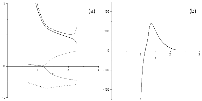
One of “non-smooth” solutions indicated above is the case of nonstandard singularity. This is the case when sometime during the evolution $\dot{H}_{i}$ diverges while $H_{i}$ remain finite. Solving eqs.(2) with respect to $\dot{H}_{i}$ we can express them in the form of fraction, and the nonstandard singularity occurs when the denominator crosses zero while numerator is regular and non-zero. In Fig. 2 the behavior of our model is shown for this case. In panel (a) we present the Hubble functions $H_{i}(t)$, in panel (b) — the behavior of the denominator of the fractional expression for $\dot{H}_{i}$. At $t\approx 1.2$ the denominator crosses zero, numerator and Hubble parameters remain regular and non-zero. As this singularity is weak according to the Tipler terminology Tipler , our numerical program typically goes through it, and the numerical results after the singularity are not physically valid: despite $H_{i}(t)$ are regular, $\dot{H}_{i}(t)$ are singular, and, hence, scalar curvature invariants diverge, which makes the non-standard singularity physical, but not a coordinate one. So, the evolution presented in Fig. 2 (a) is only valid till the point $t\approx 1.2$ where the non-standard singularity occurs. Depending on initial conditions, the nonstandard singularity can be found either in future or past history of the particular Universe. These trajectories take up to 15$\%$ of all the trajectories.

Figure 3: Typical behavior of the model which experiences a recollaps. In (a) we present the behavior of $H_{i}(t)$, in (b)— the expansion rate $\sum\limits_{i}H_{i}(t)$, in (c)—the Kasner exponents $p_{i}(t)$; $\dot{H}_{i}(t)$ in (d) and their denominator in (e).

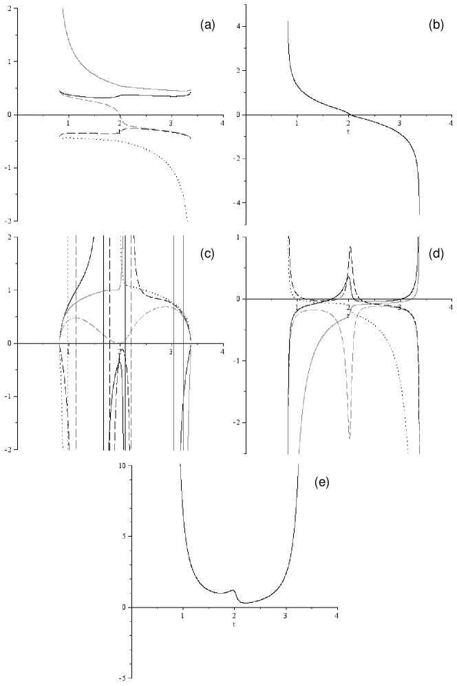
Finally, the last case is the recollaps. In this case, starting from expansion (the initial conditions in this case are chosen in a way to ensure $\sum\limits_{i}H_{i}>0$ from the beginning), the Universe begins to contract at some point and ends up in a singularity. In Fig. 3 we presented a typical behavior of the model which experience recollaps. In the panel (a) we showed individual $H_{i}(t)$, their sum in (b), individual $p_{i}(t)$ in (c). They diverge at some points due to the definition of $p_{i}$: $p_{i}=-H_{i}^{2}/\dot{H}_{i}$. In the panel (d) we presented $\dot{H}_{i}(t)$ and one can verify zeros of $\dot{H}_{i}(t)$ correspond to “singularities” of $p_{i}(t)$. Also in panel (e) of the Fig. 3 we presented the denominator of the $\dot{H}$, so the reader can verify that singularities in $p_{i}$ have nothing to do with the nonstandard singularity described above. Last thing to mention, this case occupy remaining 25$\%$ of all the trajectories.

We have considered dynamics of a flat anisotropic vacuum ($5+1$)-dimensional Universe in Gauss-Bonnet gravity. Unlike the ($4+1$)-dimensional case studied earlier s_ind , we have found that nonstandard singularity and possible recollaps which usually prevented five-dimensional Universe from reaching a low-curvature regime do not dominate in six dimensions. About 60% of trajectories in the latter case show smooth transition from GB dominated epoch to a low-curvature six-dimensional Kasner regime. The other possibilities are a “non-standard” singularity (about 15%) and a recollaps (about 25%). As we have used random set of initial conditions, other realizations can show slightly different numbers. However, our main result has a qualitative character and could not change significantly — a transition from Big Bang to low-curvature asymptotic is rather general in ($5+1$) dimensions in contrast to the ($4+1$)-dimensional case. This may indicate that Lovelock cosmology in the world with odd number of space dimensions is much less pathological than in even-dimensional worlds.

Some dynamical features of the model still require additional investigation. Another possible direction of future work is to include a matter into analysis, which can modify the results for both ($4+1$)- and ($5+1$)-dimensional cases.

References

- (1) D. Lovelock, J. Math. Phys. 12, 498 (1971).
- (2) S. Nojiri, S. Odintsov and S. Ogushi, Int. J. Mod. Phys. A17, 4809 (2002).
- (3) T.Torii and H.Maeda, Phys. Rev. D71:124002 (2005).
- (4) T.Torii and H.Maeda, Phys. Rev. D72:064007 (2005).
- (5) H.Maeda, Phys. Rev. D73:104004 (2006).
- (6) M.Aiello, R.Ferraro and G.Giribet, Class. Quant. Grav. 22, 2579 (2005).
- (7) J.Grain, A.Barrau and P.Kanti, Phys.Rev. D72: 104016 (2005).
- (8) M.Nozawa and H.Maeda, Class. Quant. Grav. 23, 1779 (2006).
- (9) R. Cai and N.Ohta Phys. Rev. D74:064001 (2006).
- (10) C.Garraffo and G.Giribet, Mod. Phys. Lett. A23, 180 (2008).
- (11) M.Dehghani and N.Farhangkhah, Phys. Rev. D78:064015 (2008).
- (12) M.Dehghani, N.Bostani and S.Hendi, Phys. Rev. D78:064031 (2008).
- (13) A.Paranjape, S.Sarkar and T.Padmanabhan, Phys.Rev. D74:104015 (2006).
- (14) N.Deruelle, Nucl. Phys. B327, 253 (1989).
- (15) N.Deruelle and J.Madore ”Kaluza-Klein cosmology with the Lovelock Lagrangian” In: Liege 1986 Proceedings, Origin and early history of the Universe, p.277-284.
- (16) N.Deruelle and L.Farina-Busto, Phys. Rev. D41, 3696 (1990).
- (17) T.Kitaura and J.Wheeler, Phys.Rev. D48, 667 (1993).
- (18) S.Kawai and J.Soda, Phys. Rev. D59:063506 (1999).
- (19) H.Yajima, K.-I. Maeda and H.Okubo, Phys. Rev. D62:034020 (2000).
- (20) A.Toporensky and S.Tsujikawa, Phys. Rev. D65:123509 (2002).
- (21) S.Alexeyev, A.Toporensky and V.Ustiansky, Phys. Lett. B509, 151 (2001).
- (22) R. Chingangban, M. Sami, P. V. Tretyakov, and A. V. Toporensky, Phys. Lett. B661, 162 (2008).
- (23) A. Toporensky and P. Tretyakov, Grav. Cosmol. 13, 207 (2007).
- (24) F.J.Tipler, Phys. Lett. A64, 8 (1977).