Real space renormalization group approach to the two-dimensional antiferromagnetic Heisenberg model (I) - The singlet triplet gap.

Abstract

The low energy behaviour of the two-dimensional antiferromagnetic Heisenberg model is studied in the sector with total spins $S=0,1,2$ by means of a renormalization group procedure, which generates a recursion formula for the interaction matrix $\Delta_{S}^{(n+1)}$ of 4 neighbouring “$n$ clusters” of size $2^{n}\times 2^{n}$, $n=1,2,3,\ldots$ from the corresponding quantities $\Delta_{S}^{(n)}$. Conservation of total spin $S$ is implemented explicitly and plays an important role. It is shown, how the ground state energies $E_{S}^{(n+1)}$, $S=0,1,2$ approach each other for increasing $n$, i.e. system size. The most relevant couplings in the interaction matrices are generated by the transitions $\langle S^{\prime},m^{\prime};n+1|S_{q}^{*}|S,m;n+1\rangle$ between the ground states $|S,m;n+1\rangle$ ($m=-S,\ldots,S$) on an $(n+1)$-cluster of size $2^{n+1}\times 2^{n+1}$, mediated by the staggered spin operator $S_{q}^{*}$.

I Introduction

The discovery of high $T_{c}$ superconductors 20 years ago bednorz86 led to an intensive search for new mechanisms, which could explain the observed superconductivity in $CuO_{2}$ planes. It became clear very soon, that two ingredients are needed, holes in low concentration which move in a $2D$ antiferromagnetic background. The Hubbard modelhubbard63 and the $t-J$ modelanderson87 have been discussed in this context. If the hopping of holes is frozen in, these models reduce to the Heisenberg model with Hamiltonian

$$H = \sum_{\langle x,y\rangle}{\bf S}(x){\bf S}(y)$$ (1)

where $S_{i}(x)$, $i=1,2,3$ denote spin $1/2$ operators at site $x$. In the absence of an external field (1) conserves the total spin

$${\bf S} = \sum_{x}{\bf S}(x)$$ (2)

and the ground state is known to be a singlet state ($S=0$) with momentum ${\bf p}=(0,0)$. The first excited state $|1,q\rangle$ is a triplet ($S=1,\,\,q=0,\pm 1$) with momentum ${\bf p}=(\pi,\pi)$. The transition between these two states is mediated by the staggered spin operator

$$S_{q}^{*} = \sum_{x}(-1)^{x}S_{q}(x)\hskip 22.76228ptq=0,\pm 1$$ (3)

$$S_{0}(x) = \frac{1}{2}\sigma_{3}(x)\,,\hskip 17.07182ptS_{\pm}(x)=\frac{1}{2\sqrt{2}}\Big{(}\sigma_{1}(x)\pm i\sigma_{2}(x)\Big{)}$$

and the matrix element

$$m^{*} = \frac{1}{N}\langle 1q|S_{q}^{*}|0\rangle$$ (5)

can be considered as an order parameter.

The ground state properties of the $2D$ Heisenberg model (1) have been investigated with various methods. The variational $RVB$-state baskaran87 (“Resonating Valence Bond”) starts from singlet states on pairs of sites, which cover the whole $2D$ lattice. By construction, these states lead to eigenstates of the total spin ${\bf S}$ with $S=0$. However, the manifold of these states which can be constructed is nonorthogonal and overcomplete.

Numerical methods - e.g. the Lanczos algorithm - are limited to small clusters $N\leq 6\times 6=36$ due to storage problems. The computation on the largest cluster $6\times 6$ has been performed by Schulz and Zimanschulz92 15 years ago.

In spite of the great improvements achieved during this time, it is not possible so far to repeat the calculation of Schulz and Ziman for the next interesting cluster $8\times 8$. This is only possible with other techniques, as the quantum Monte Carlo [cf. e.g. (manousakis91, )].

Our approach to the low energy properties of the two-dimensional antiferromagnetic Heisenberg model starts from a decomposition of the lattice into plaquettes as depicted in Fig. 1. Quantum numbers, energies and couplings for plaquette states are discussed in Section II. In particular we find, that the lowest energy plaquette states with total spin $S=0$ (singlet), $S=1$ (triplet), $S=2$ (quintuplet) appear to be most important for the construction of the ground states on larger clusters. This is demonstrated in Section III where we compose 4 plaquettes to a $4\times 4$ cluster with open boundary conditions (cf. Fig. 2). We deduce interaction matrices from the couplings between neighbouring plaquettes for the $4\times 4$ system in the sectors with total spin $S=0,1,2$. The diagonalization of these interaction matrices yield predictions for energies and transition matrix elements, which can be compared with Lanczos results on a $4\times 4$ system. We find agreement within $1-6\%$, depending on the quantity under consideration.

In a next step, described in Section IV, we generalize this approach to larger “$n$-clusters” of size $2^{n}\times 2^{n}$, $n=2,3,4,\ldots$. E.g. the $n=3$ cluster of size $8\times 8$ is composed from four $n=2$ clusters ($4\times 4$). Each of these clusters can be occupied with a cluster ground state with total spin $S$ ($S=0,1,2$). The interaction matrix for the $n+1$-clusters have the same structure as in the step before - i.e. for $n$-clusters. The $n$-dependence can be absorbed in a renormalization of couplings and gaps, which is discussed in Sections V and VI. The numerical evaluation of the renormalization group equations is discussed in Section VII. Section VIII is devoted to the treatment of the staggered magnetization in our approach.

Let us finally mention, that the idea to describe the ground state properties of the antiferromagnetic Heisenberg model in the framework of a renormalization group approach is not new. One of the first attempts in this direction has been presented already in 1992 by Lin and Campbell.lin92 ; lin94 They started from $L\times L$ clusters with $L$ odd ($L=3,5$) and computed the ground state (which has total spin 1/2) and its interaction with sites on a ring. In this way, they were able to make a prediction for the staggered magnetization on a $7\times 7$ lattice.

There have been many investigations of ordered antiferromagnets, which start from the observation that the dominant fluctuations are controlled by the quantum nonlinear $\sigma$-model with imaginary time. chakravarty88 ; fisher89 ; affleck86 ; affleck87

The various renormalization group approaches differ in the clusters used and in the truncation of the Hilbert space, which is needed to make the evaluation feasible. This is discussed in Section IX.

II Plaquette states: Quantum numbers, energies and couplings

Our approach to the $2D$ antiferromagnetic Heisenberg model starts with a decomposition of the $2D$ lattice into plaquettes as depicted in Fig. 1.

Figure 1: 4-plaquette system with $2^{n}\times 2^{n}=4\times 4$ sites – here $n=2$; the single plaquette on the right shows the enumeration of plaquette sites.

Each plaquette can carry 16 eigenstates. Their quantum numbers and energies are listed in Table 1.

	$|0\rangle$	$|A_{q}\rangle$	$|B_{q}\rangle$	$|C_{q}\rangle$	$|\hat{0}\rangle$	$|Q_{r}\rangle$
$S(P)$	0	1	1	1	0	2
$S_{z}(P)$	0	$q=\pm 1,0$	$q=\pm 1,0$	$q=\pm 1,0$	0	$r=\pm 2,\pm 1,0$
$E(P)$	-2	-1	0	0	0	1

Table 1: Quantum numbers of the 16 plaquette states.

The spin quantum numbers $S(P)$ in the first row result from a decomposition of the 4 spins into irreducible representations of the $SU(2)$. In this way we get two singlets $|0\rangle$, $|\hat{0}\rangle$ with energies $E_{0}=-2$, $E_{\hat{0}}=0$, three triplets $|Aq\rangle$, $Bq\rangle$, $|Cq\rangle$ with energies $E_{A}=-1$, $E_{B}=E_{C}=0$ and one quintuplet $|Q_{r}\rangle$ with energy $E_{2}=1$.

The ground state $|0\rangle$ is given by the following spin configuration on the plaquette

$$|0\rangle = \frac{1}{\sqrt{12}}\left\{\left(\begin{array}[]{cc}+&+\\ -&-\end{array}\right)+\left(\begin{array}[]{cc}-&-\\ +&+\end{array}\right)+\left(\begin{array}[]{cc}+&-\\ +&-\end{array}\right)+\right.$$ (14)

$$\left.\hskip 25.6073pt\left(\begin{array}[]{cc}-&+\\ -&+\end{array}\right)-2\left(\begin{array}[]{cc}+&-\\ -&+\end{array}\right)-2\left(\begin{array}[]{cc}-&+\\ +&-\end{array}\right)\right\}\,.$$

The three triplet states are obtained

$$|i,q\rangle = S_{q}^{(i)}|0\rangle\frac{1}{\langle 0|S_{-q}^{(i)}S_{q}^{(i)}|0\rangle^{1/2}}\quad i=A,B,C\quad\quad$$ (16)

by application of the plaquette spin operators

$$S_{q}^{(i)} = \sum_{x\in P}\chi^{(i)}(x)S_{q}(x)\quad q=0,\pm 1\quad i=A,B,C$$

on the ground state (LABEL:GS_0). The signs $\chi^{(i)}(x)$

$$\chi^{(A)}(x)=(+-+-), \chi^{(B)}(x)=(++--),\quad$$

$$\chi^{(C)}(x)=(+--+)\,$$ (18)

define the magnetic order of triplet states on the plaquette:

$|A_{q}\rangle$ is antiferromagnetic in the sense, that it changes sign running around the plaquette

$|B_{q}\rangle$ and $|C_{q}\rangle$ are collinear antiferromagnetic in horizontal and vertical direction, respectively.

The tensor states $|Q_{r}\rangle$, $r=-2,-1,0,1,2$ are totally symmetric with respect to the four sites of the plaquette.

The simplest variational ansatz on the $2D$ lattice would start from a product state where all plaquettes are occupied with singlets. Such an ansatz would lead to an energy per plaquette $E_{0}(P)=-2$ which is just $75\%$ of the “exact” value

$$\hat{E}_{0} = 4\cdot(-0.668)=-2.674$$ (19)

as it follows for the thermodynamical limit from a finite-size scaling analysis [Husehuse88 (1988)]. Recent quantum Monte Carlo calculations [Sandviksandvik97 (1997), Loewloew07 (2007)] improve the ground state energy to $e_{0}=0.669437(5)$.

Therefore the interaction between neighbouring plaquettes $P_{l}$ $P_{r}$ - as depicted in Fig. 2 - has to account for 25$\%$ of the ground state energy.

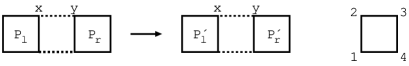
Figure 2: Interaction of neighbouring plaquettes.

If the two neighbouring plaquettes carry spins $|S_{l},m_{l}\rangle$, $|S_{r},m_{r}\rangle$ $S=0,1,2$, $m=-S,\ldots,S$ the spin interaction term ${\bf S}(x){\bf S}(y)$ at two neighbouring sites $x\in P_{l}$, $y\in P_{r}$ induces a change in the spin quantum numbers

$$|S_{l},m_{l}\rangle\begin{array}[]{c}{\bf S}(x)\\ \longrightarrow\end{array}|S^{\prime}_{l},m^{\prime}_{l}\rangle |S_{r},m_{r}\rangle\begin{array}[]{c}{\bf S}(y)\\ \longrightarrow\end{array}|S^{\prime}_{r},m^{\prime}_{r}\rangle\,.$$ (24)

The transition matrix element

$$\langle S^{\prime}_{l},m^{\prime}_{l}|S_{q}(x)|S_{l},m_{l}\rangle = v_{q}\left(\begin{array}[]{c|cc}S^{\prime}_{l}&1&S_{l}\\ m^{\prime}_{l}&q&m_{l}\end{array}\right)M(S^{\prime}_{l},x,S_{l})$$ (28)

can be evaluated by means of the Wigner-Eckart Theorem.edmonds60 All these matrix elements can be expressed in terms of a Clebsch-Gordan coefficient and one reduced matrix element $M(S^{\prime}_{l},x,S_{l})$. The latter only depends on the initial and final plaquette spins $S_{l}$ and $S^{\prime}_{l}$ and the triplet operator $S_{q}(x)$ at site $x$. The phase $v_{q}$ ($v_{+}=-1$, $v_{0}=v_{-}=1$) results from the transformation properties of the spin operator $S_{q}(x)$ under the group $SU(2)$. The interaction between neighbouring plaquettes then depends on the product of two Clebsch-Gordan coefficients

$$v_{q}v_{q}\left(\begin{array}[]{c|cc}S^{\prime}_{l}&1&S_{l}\\ m^{\prime}_{l}&q&m_{l}\end{array}\right)\left(\begin{array}[]{c|cc}S^{\prime}_{r}&1&S_{r}\\ m^{\prime}_{r}&q&m_{r}\end{array}\right)\overline{M}(S^{\prime}_{l},S_{l};S^{\prime}_{r},S_{r})$$ (34)

(35)

and the product of reduced matrix elements

$$\overline{M}(S^{\prime}_{l},S_{l};S^{\prime}_{r},S_{r}) = \sum_{\langle x,y\rangle}M(S^{\prime}_{l},x,S_{l})M(S^{\prime}_{r},y,S_{r})\quad\quad$$

(36)

summed over the two neighbouring sites $\langle x,y\rangle$, which connect the left and right plaquette as shown in Fig. 2. The Clebsch-Gordan coefficients lead to selection rules

$$S^{\prime}_{l} = S_{l}\pm 1,S_{l}\hskip 35.56593pt\mbox{for }S_{l}\geq 1$$

$$S^{\prime}_{l} = 1\hskip 62.59596pt\mbox{for }S_{l}=0$$

$$m^{\prime}_{l} = m_{l}+q\,.$$

The explicit calculation of the transition matrix elements yields the weights $\overline{M}(S^{\prime}_{l},S_{l};S^{\prime}_{r},S_{r})$ for the following cases:

1. Creation of triplet pairs from singlet pairs

   $$0\quad 0 \leftrightarrow A_{q}\quad A_{-q}$$ (38)

   Note, that the initial and final states have total spin 0. According to (35) and (36) the weight for this process turns out to be

   $$\sum_{q}\left(\begin{array}[]{c|cc}1&1&0\\ q&q&0\end{array}\right)\left(\begin{array}[]{c|cc}1&1&0\\ -q&-q&0\end{array}\right)\overline{M}^{(1)}(10,10)$$ (43)

   where

   $$\overline{M}^{(1)}(10,10) = a^{(1)}=-\frac{1}{3}\,.$$ (45)

2. Hopping of an isolated triplet on a singlet background

   $$0\quad A_{q} \leftrightarrow A_{q}\quad 0\quad q=\pm 1,0$$ (46)

   Here, the initial and final states are triplets on different plaquettes ($P_{r}$ and $P_{l}$). The corresponding weight is given again by (45).

3. The triplet-triplet process

   $$A_{s+q}\quad A_{t-q} \leftrightarrow A_{s}\quad A_{t}\quad q=\pm 1,0$$ (47)

   introduces a new weight:

   $$(-)^{q}\left(\begin{array}[]{c|cc}1&1&1\\ s+q&q&s\end{array}\right)\left(\begin{array}[]{c|cc}1&1&1\\ t-q&-q&t\end{array}\right)\overline{M}^{(1)}(11,11)\,.$$ (52)

   (53)

   where

   $$\overline{M}^{(1)}(11,11) = \frac{1}{4}\,.$$ (54)

4. The process

   $$Q_{r}\quad 0 \leftrightarrow A_{r-q}\quad A_{q}$$ (55)

   starts from an initial state with a spin 2 plaquette $Q_{r}$ and a spin 0 plaquette (singlet). In the final state we have two triplets $A_{r-q}$ $A_{q}$ coupled with an appropriate Clebsch-Gordan coefficient to form again a spin 2 state. The coupling for (55) turns out to be

   $$\left(\begin{array}[]{c|cc}2&1&1\\ r&q&r-q\end{array}\right)\left(\begin{array}[]{c|cc}1&1&0\\ q&q&0\end{array}\right)\overline{M}(21,10)$$ (60)

   where

   $$\overline{M}^{(1)}(21,10) = \frac{1}{2\sqrt{3}}\,.$$ (61)

5. The process

   $$Q_{r}\quad A_{-q} \leftrightarrow A_{r-q}\quad 0$$ (62)

   describes the transition from a spin 2 - spin 1 to a spin 1 spin 0 plaquette. It is accompanied with a weight

   $$(-)^{q}\left(\begin{array}[]{c|cc}2&1&1\\ r&q&r-q\end{array}\right)\left(\begin{array}[]{c|cc}1&1&0\\ -q&-q&0\end{array}\right)\overline{M}^{(1)}(21,10)\,.$$ (67)

6. The exchange of a spin 2 - spin 1 plaquette

   $$Q_{r}\quad A_{p} \leftrightarrow A_{r-q}\quad Q_{p+q}$$ (69)

   carries a weight

   $$\left(\begin{array}[]{c|cc}2&1&1\\ r&q&r-q\end{array}\right)\texttwosuperior\left(\begin{array}[]{c|cc}2&1&1\\ p+q&q&p\end{array}\right)\texttwosuperior\overline{M}^{(1)}(21,21)\,.$$ (74)

   where

   $$\overline{M}^{(1)}(21,21) = -\frac{1}{4}\,.$$ (76)

7. If the spin 2 - spin 1 plaquettes do not change their position

   $$Q_{r}\quad A_{p} \leftrightarrow Q_{r+q}\quad A_{p-q}$$ (77)

   the corresponding weight is:

   $$(-)^{q}\left(\begin{array}[]{c|cc}2&1&2\\ r+q&q&r\end{array}\right)\texttwosuperior\left(\begin{array}[]{c|cc}1&1&1\\ p-q&-q&p\end{array}\right)\texttwosuperior\overline{M}^{(1)}(22,11)\,.$$ (82)

   (83)

   where

   $$\overline{M}^{(1)}(22,11) = \frac{\sqrt{3}}{4}\,.$$ (84)

(45)-(83) is a complete list of processes where only singlets $|0\rangle$, $A$-triplets $|A_{q}\rangle$ and quintuplets $|Q_{r}\rangle$ are involved. In our opinion they are most important for the low energy behaviour for the following reasons:

• $|0\rangle$ and $|A_{q}\rangle$ have the lowest energies according to Table 1.

• the staggered spin operator [eq. (LABEL:staggered) for $i=A$] on the plaquette induces the dominant transitions

  $$|0\rangle\stackrel{{\scriptstyle S_{q}^{(*)}}}{{\rightarrow}}|A_{q}\rangle\stackrel{{\scriptstyle S_{r-q}^{(*)}}}{{\rightarrow}}|Q_{r}\rangle$$

  As a consequence, the weights (45), (61) and (76) which are built up from these transitions are dominant as well.

Truncating the states with subdominant transitions anticipates antiferromagnetic order of the system for the renormalization procedure. This is somewhat in analogy to treatments by spin-wave theory or mappings to nonlinear sigma models, see e.g. (hamer94, ) and (chakravarty88, ). In these approaches long-range antiferromagnetic order is assumed from the beginning and fluctuations around this is built in subsequently. In our approach however, the system may or may not develop long-range order. This is determined by the renormalization group flow.

III The four plaquette system

We are going to construct in this Section the ground states of the four plaquette system with $4\times 4$ sites depicted in Fig. 1. It turns out that the ground states are symmetric under rotation of the four plaquettes. We therefore start from rotationally symmetric basis states, which are eigenstates of the total spin squared ${\bf S}^{2}$ and its 3-component

$${\bf S} = \sum_{j=1}^{4}{\bf S}(P_{j})\,.$$ (1)

III.1 The singlet sector

In Table 2 we list 7 singlet states which can be constructed on the four plaquette system with singlets ($0$), triplets ($A_{q}$) and at most one spin 2 ($Q_{r}$) plaquette.

$|1,0\rangle=$	$\left(\begin{array}[]{cc}0&0\\ 0&0\end{array}\right)$
$|2,0\rangle=$	${\displaystyle\frac{1}{2\sqrt{3}}\sum_{q}}(-)^{q}\left\{\left(\begin{array}[]{cc}A_{q}&A_{-q}\\ 0&0\end{array}\right)+\mbox{ rot}\right\}$
$|3,0\rangle=$	${\displaystyle\frac{1}{\sqrt{6}}\sum_{q}}(-)^{q}\left\{\left(\begin{array}[]{cc}A_{q}&0\\ 0&A_{-q}\end{array}\right)+\left(\begin{array}[]{cc}0&A_{q}\\ A_{-q}&0\end{array}\right)\right\}$
$|4,0\rangle=$	${\displaystyle\frac{1}{3}\sum_{q,p}}(-)^{p+q}\left(\begin{array}[]{cc}A_{q}&A_{p}\\ A_{-p}&A_{-q}\end{array}\right)$
$|5^{\prime},0\rangle=$	${\displaystyle\sum_{q,p}}(-)^{p+q}\left\{\left(\begin{array}[]{cc}A_{-p}&A_{p}\\ A_{q}&A_{-q}\end{array}\right)+\mbox{ rot}\right\}$
$|6,0\rangle=$	${\displaystyle\frac{1}{2\sqrt{10}}\sum_{q,p}}(-)^{p+q}\left(\begin{array}[]{c|cc}2&1&1\\ r&q&p\end{array}\right)\times$
	$\left\{\left(\begin{array}[]{cc}A_{q}&A_{p}\\ Q_{-r}&0\end{array}\right)+\left(\begin{array}[]{cc}A_{q}&Q_{-r}\\ A_{p}&0\end{array}\right)+\mbox{ rot}\right\}$
$|7,0\rangle=$	${\displaystyle\frac{1}{2\sqrt{5}}\sum_{q,p}}(-)^{p+q}\left(\begin{array}[]{c|cc}2&1&1\\ r&q&p\end{array}\right)\times$
	$\left\{\left(\begin{array}[]{cc}Q_{-r}&A_{p}\\ A_{q}&0\end{array}\right)+\mbox{ rot}\right\}$

Table 2: Basis states of the 4 plaquette system in the singlet sector.

Starting from the state $|1,0\rangle$, where the four plaquettes are occupied with plaquette singlets $|0\rangle$, the creation process (38) generates the state $|2,0\rangle$ with neighbouring triplets $A_{q}A_{-q}$ coupled to a total spin 0. The hopping process (46) leads from $|2,0\rangle$ to $|3,0\rangle$. Further application of (38) and (46) generates the states $|3,0\rangle$,, $|4,0\rangle$, $|5^{\prime},0\rangle$. The first four states $|i,0\rangle$, $i=1,2,3,4$ are orthonormal. This is not the case for $|5^{\prime},0\rangle$, which is orthonormalized by

$$|5,0\rangle = N_{5}\Big{(}|5^{\prime},0\rangle-\langle 4,0|5^{\prime},0\rangle|4,0\rangle\Big{)}\,,$$ (2)

where

$$\langle 4,0|5^{\prime},0\rangle = 4$$ (3)

and

$$N_{5} = \frac{1}{4\sqrt{5}}\,.$$ (4)

The states $|6,0\rangle$ and $|7,0\rangle$ contain one spin 2 plaquette $Q_{r}$ coupled together with two spin 1 plaquettes $A_{q}$ $A_{p}$ to form a state with total spin 0. The states $|i,0\rangle$ $i=1,2,..,7$ are orthonormal and complete in the sense, that no further rotational symmetric state can be constructed from plaquette singlets, triplets and one quintuplet. The Hamiltonian restricted to the Hilbert space of these seven singlet states can be written as

$$H_{0}^{(2)} = 4E_{0}^{(1)}+a^{(1)}\Delta_{0}^{(2)}\,.$$ (5)

The first term is just the energy of the state $|1,0\rangle$. We have scaled out the singlet-triplet coupling (45). The remaining “interaction matrix” $\Delta_{0}^{(2)}$ is listed in Appendix A.1.

The following remarkable features can be observed in the interaction matrix $\Delta_{0}^{(2)}$:

1. The nondiagonal matrix elements are nonnegative and fixed by the weights

   $$a^{(1)}=\overline{M}^{(1)}(10;10) = -\frac{1}{3}$$ (6)

   $$\gamma^{(1)}=\frac{\overline{M}^{(1)}(21;10)}{\overline{M}^{(1)}(10;10)} = -\frac{\sqrt{3}}{2}$$ (7)

   They are induced by the singlet-triplet $(1,0)$ and triplet-quintuplet $(2,1)$ transition matrix elements according to (36).

   Therefore, the Perron-Frobenius theorem holds, which states that the eigenvectors $|\sigma^{(2)}\rangle$ with largest eigenvalue $\sigma^{(2)}$:

   $$\Delta_{0}^{(2)}|\sigma^{(2)}\rangle = \sigma^{(2)}|\sigma^{(2)}\rangle$$ (8)

   $$\sigma^{(2)} = 2.20917$$ (9)

   have nonnegative components:

   $$\langle i,0|\sigma^{(2)}\rangle \geq 0\quad i=1,...,7\,.$$ (10)

2. The triplet-triplet and quintuplet-quintuplet transition matrix elements, which define the weights

   $$\beta^{(1)} = \frac{M^{(1)}(11;11)}{a^{(1)}}=-\frac{3}{4}$$ (11)

   $$\varepsilon^{(1)} = \frac{M^{(1)}(22;11)}{a^{(1)}}=-\frac{3\sqrt{3}}{4}$$ (12)

   only contribute to the diagonal matrix elements. They also depend on the two scaled gaps

   $$\rho=\rho^{(1)} = \frac{1}{a^{(1)}}\Big{(}E_{1}^{(1)}-E_{0}^{(1)}\Big{)}=-3$$ (13)

   $$\kappa=\kappa^{(1)} = \frac{1}{a^{(1)}}\Big{(}E_{2}^{(1)}+E_{0}^{(1)}-2E_{1}^{(1)}\Big{)}=-3$$ (14)

   $$\,.$$

3. The ground state energy of the Hamiltonian (5) in the restricted Hilbert space of the singlet states $|j,0\rangle$, $j=1,...,7$ is given by

   $$E_{0}^{(2)} = 4E_{0}^{(1)}+a^{(1)}\sigma^{(2)}=-8.7236$$ (15)

   which deviates from the “exact´´ value for the $4\times 4$ system with open b.c.

   $$E_{0}^{(L)} = -9.1892$$ (16)

   by $5.0\%$.

III.2 The triplet sector

$|1,+\rangle=$	${\displaystyle\frac{1}{\sqrt{4}}}\left\{\left(\begin{array}[]{cc}A_{+}&0\\ 0&0\end{array}\right)+\mbox{ rot}\right\}$
$|2,+\rangle=$	${\displaystyle\frac{1}{2\sqrt{3}}\sum_{q}}(-)^{q}\left\{\left(\begin{array}[]{cc}A_{+}&A_{q}\\ A_{-q}&0\end{array}\right)+\mbox{ rot}\right\}$
$|3^{\prime},+\rangle=$	${\displaystyle\sum_{q}}(-)^{q}\left\{\left(\begin{array}[]{cc}A_{+}&A_{q}\\ 0&A_{-q}\end{array}\right)+\left(\begin{array}[]{cc}A_{q}&A_{-q}\\ 0&A_{+}\end{array}\right)+\mbox{ rot}\right\}$
$|4,+\rangle=$	${\displaystyle\frac{1}{2\sqrt{2}}\sum_{q}}\left(\begin{array}[]{c|cc}1&2&1\\ 1&1-q&q\end{array}\right)\times$
	$\hskip 31.2982pt\left\{\left(\begin{array}[]{cc}Q_{1-q}&A_{q}\\ 0&0\end{array}\right)+\left(\begin{array}[]{cc}Q_{1-q}&0\\ A_{q}&0\end{array}\right)+\mbox{ rot}\right\}$
$|5,+\rangle=$	${\displaystyle\frac{1}{\sqrt{4}}\sum_{q}}\left(\begin{array}[]{c|cc}1&2&1\\ 1&1-q&q\end{array}\right)\left\{\left(\begin{array}[]{cc}Q_{1-q}&0\\ 0&A_{q}\end{array}\right)+\mbox{ rot}\right\}$
$|k,+\rangle=$	${\displaystyle\frac{1}{\sqrt{4}}\sum_{p,q,r}}C_{-r,-p,-q}^{J,j}\times\left\{\left(\begin{array}[]{cc}Q_{r+1}&A_{-p}\\ A_{-q}&A_{-r+p+q}\end{array}\right)+\mbox{ rot}\right\}$
with:
	$C_{-r,-p,-q}^{J,j}=\left(\begin{array}[]{c|cc}j&1&1\\ -p-q&-p&-q\end{array}\right)\times$
	$\left(\begin{array}[]{c|cc}J&j&1\\ -r&-p-q&-r+p+q\end{array}\right)\left(\begin{array}[]{c|cc}1&2&J\\ 1&r+1&-r\end{array}\right)$
and:	$\,k\,$  6  7  8 9 $j$ 0 2 2 2 $J$ 1 1 2 3

Table 3: Basis states of the 4 plaquette system in the triplet sector.

The rotational symmetric eigenstates of the 4 plaquette system in the sector with total spin $S=1$ are listed in Table 3:

Starting from $|1,+\rangle$, we generate the other states $|3^{\prime},+\rangle$, $|2,+\rangle$, $|4,+\rangle$ and $|5,+\rangle$ by means of the processes (38) (46) and (55). The states $|1,+\rangle$, $|2,+\rangle$, $|4,+\rangle$, $|5,+\rangle$ are orthonormal. The state $|3^{\prime},+\rangle$ is not yet orthonormal with respect to $|2,+\rangle$, which is achieved by:

$$|3,+\rangle = N_{3}\Big{(}|3^{\prime},+\rangle-\langle 2,+|3^{\prime},+\rangle|2,+\rangle\Big{)}\,,$$ (17)

with

$$\langle 2,+|3^{\prime},+\rangle = \frac{4}{\sqrt{3}}$$ (18)

and

$$N_{3} = \frac{\sqrt{3}}{4\sqrt{5}}\,.$$ (19)

The states $|k,+\rangle$, $k=6,7,8,9$ contain one spin-2 and three spin-1 plaquettes, which are coupled together with appropriate Clebsch-Gordan coefficients ($C_{-r,-p,-q}^{J,j}$) eigenstates with total spin 1. There exist two further states ($j=1$, $J=1,2$) that do not couple to the considered ones.

The Hamiltonian in the restricted Hilbert space of the states $|k,+\rangle$ $k=1,\ldots,9$ reads

$$H_{1}^{(2)} = 3E_{0}^{(1)}+E_{1}^{(1)}+a^{(1)}\Delta_{1}^{(2)}\,.$$ (20)

The first term is the energy of the lowest state $|1,+\rangle$. Again we have scaled out the singlet-triplet coupling $a^{(1)}$ (6), such that the interaction matrix $\Delta_{1}^{(2)}$ depends on the two scaled gaps $\rho^{(1)}$ (13), $\kappa^{(1)}$ (14) and the three scaled couplings $\gamma^{(1)}$ (7), $\beta^{(1)}$ (11) and $\varepsilon^{(1)}$ (12). Diagonalizing the interaction matrix:

$$\Delta_{1}^{(2)}|\tau^{(2)}\rangle = \tau^{(2)}|\tau^{(2)}\rangle$$ (21)

yields the largest eigenvalue

$$\tau^{(2)} = 3.41009$$ (22)

which corresponds to a ground state energy

$$E_{1}^{(2)} = -7-\frac{\tau^{(2)}}{3}=-8.18405\,.$$ (23)

The latter deviates from the Lanczos result on a $4\times 4$ system with open b.c.

$$E_{1}^{(L)} = -8.6869..$$ (24)

by $6.3\%$.

III.3 The spin 2 sector

The 14 basis states $|l,2+\rangle$ for the 4-plaquette system (Fig. 1) in the spin 2 sector are listed in Table 4

The states $|l,2+\rangle$, $l=1,2,3,5$ are orthonormal, which is not the case for $|4^{\prime},2+\rangle$ with respect to $|3,2+\rangle$. We therefore introduce

$$|4,2+\rangle = N_{4}\Big{(}|4^{\prime},2+\rangle-\langle 3,2+|4^{\prime},2+\rangle|3,2+\rangle\Big{)}$$

with

$$\langle 3,2+|4^{\prime},2+\rangle = \frac{4\sqrt{2}}{\sqrt{3}}$$ (26)

$$N_{4} = \frac{\sqrt{3}}{2\sqrt{7}}$$ (27)

The states $|6+j,2+\rangle$, $|9+j,2+\rangle$ and $|12+j,2+\rangle$ contain one spin 2 and two spin 1 plaquettes - the latter are coupled together to a state with spin $j$, which then forms with the $Q_{r}$ plaquette a state with total spin 2.

In the restricted Hilbert space of the states $|l,2+\rangle$, $l=1,\ldots,14$ the Hamiltonian can be written as

$$H_{2}^{(2)} = 2(E_{0}^{(1)}+E_{1}^{(1)})+a^{(1)}\Delta_{2}^{(2)}\,.$$ (28)

Again the first term corresponds to the plaquette energies of the state $|1,2+\rangle$ (and $|2,2+\rangle$). The interaction matrix $\Delta_{2}^{(2)}$ depends on the scaled gaps $\rho^{(1)}$ (13), $\kappa^{(1)}$ (14) and the three scaled couplings $\gamma^{(1)}$ (7), $\beta^{(1)}$ (11) and $\varepsilon^{(1)}$ (12), as can be seen in Appendix A.3.

$|1,2+\rangle=$	${\displaystyle\frac{1}{\sqrt{4}}}\left\{\left(\begin{array}[]{cc}A_{+}&A_{+}\\ 0&0\end{array}\right)+\mbox{ rot}\right\}$
$|2,2+\rangle=$	${\displaystyle\frac{1}{\sqrt{2}}}\left\{\left(\begin{array}[]{cc}A_{+}&0\\ 0&A_{+}\end{array}\right)+\left(\begin{array}[]{cc}0&A_{+}\\ A_{+}&0\end{array}\right)\right\}$
$|3,2+\rangle=$	${\displaystyle\sum_{q}\frac{(-)^{q}}{\sqrt{6}}}\Bigg{\{}\left(\begin{array}[]{cc}A_{+}&A_{q}\\ A_{-q}&A_{+}\end{array}\right)+\left(\begin{array}[]{cc}A_{q}&A_{+}\\ A_{+}&A_{-q}\end{array}\right)\Bigg{\}}$
$|4^{\prime},2+\rangle=$	${\displaystyle\sum_{q}}(-)^{q}\Bigg{\{}\left(\begin{array}[]{cc}A_{+}&A_{+}\\ A_{q}&A_{-q}\end{array}\right)+\mbox{ rot}\Bigg{\}}$
$|5,2+\rangle=$	${\displaystyle\frac{1}{\sqrt{4}}}\left\{\left(\begin{array}[]{cc}Q_{2+}&0\\ 0&0\end{array}\right)+\mbox{ rot}\right\}$
$|6+j,2+\rangle=$	${\displaystyle\frac{1}{\sqrt{4}}\sum_{q,p}}C_{p,q}^{j}\left\{\left(\begin{array}[]{cc}A_{-p}&0\\ Q_{r+2}&A_{-q}\end{array}\right)+\mbox{ rot}\right\}$
$|9+j,2+\rangle=$	${\displaystyle\frac{1}{\sqrt{4}}\sum_{q,p}}C_{p,q}^{j}\left\{\left(\begin{array}[]{cc}A_{-q}&A_{-p}\\ Q_{r+2}&0\end{array}\right)+\mbox{ rot}\right\}$
$|12+j,2+\rangle=$	${\displaystyle\frac{(-)^{j}}{\sqrt{4}}\sum_{q,p}}C_{p,q}^{j}\left\{\left(\begin{array}[]{cc}0&A_{-p}\\ Q_{r+2}&A_{-q}\end{array}\right)+\mbox{ rot}\right\}$
	$C_{p,q}^{j}=\left(\begin{array}[]{c|cc}2&2&j\\ 2&2+r&-r\end{array}\right)\left(\begin{array}[]{c|cc}j&1&1\\ -r&-q&-p\end{array}\right)$
	$\hskip 62.59596ptj=0,1,2;\quad r=p+q$

Table 4: Basis states of the 4 plaquette system in the quintuplet sector.

Diagonalizing the interaction matrix

$$\Delta_{2}^{(2)}|\xi^{(2)}\rangle = \xi^{(2)}|\xi^{(2)}\rangle$$ (29)

yields the largest eigenvalue

$$\xi^{(2)} = 3.48987$$ (30)

which corresponds to a ground state energy

$$E_{2}^{(2)} = -6-\frac{\xi^{(2)}}{3}=-7.36767\,.$$ (31)

The latter deviates from the Lanczos result on a $4\times 4$ system with open b.c.

$$E_{2}^{(L)} = -7.7909..$$ (32)

by $8.0\%$.

IV The renormalization group procedure

In the previous Section we have explained how to construct the ground state on a ($n=2$) cluster of size $4\times 4$ from four interacting $n=1$ plaquettes ($2\times 2$). We only took into account plaquette states with total spin 0, 1 and 2. This procedure will now be extended to compute the ground states on ($n+1$) clusters ($2^{n+1}\times 2^{n+1}$) with total spin $S=0,1,2$ from the corresponding quantities on $n$ clusters. The ground states

$$|S,m;n+1\rangle S=0,1,2,m=-S,\ldots S$$ (33)

are supposed to carry alternating momenta

$${\bf p}_{S}=(0,0) S=0,2$$ for

$${\bf p}_{S}=(\pi,\pi) S=1\,.$$ for

Our approach starts from the basic assumption, that the ground state (33) on ($n+1$) clusters can be constructed from the ground state on $n$ clusters

$$|S^{\prime},m^{\prime};n\rangle S=S^{\prime}+1,S^{\prime},S^{\prime}-1\hskip 14.22636ptS^{\prime}\geq 1$$

$$S=1,0\hskip 71.13188ptS^{\prime}=0$$

Under this assumption the Hamiltonians $H_{S}^{(n+1)}$ on the $(n+1)$ cluster ($2^{n+1}\times 2^{n+1}$) can be written in an analogous form to (5) for $S=0$, (20) for $S=1$ and (28) for $S=2$. To be definite, we introduce first the analogues of the basis states in Tables 2, 3, 4:

$$|i,0;n+1\rangle i=1,\ldots 7$$ (36)

$$|k,+;n+1\rangle k=1,\ldots 9$$ (37)

$$|l,2+;n+1\rangle l=1,\ldots 14$$ (38)

on a $(n+1)$ block ($2^{n+1}\times 2^{n+1}$).

Then the analogues of the interaction matrices $\Delta_{0}^{(n+1)}$ are obtained from Appendix A by substituting the scaled energy gaps and couplings

$$\rho=\rho^{(n)} = \frac{E_{1}^{(n)}-E_{0}^{(n)}}{a^{(n)}}$$ (39)

$$\kappa=\kappa^{(n)} = \frac{E_{2}^{(n)}+E_{0}^{(n)}-2E_{1}^{(n)}}{a^{(n)}}$$ (40)

$$a=a^{(n)} = \overline{M}^{(n)}(10;10)$$ (41)

$$\gamma=\gamma^{(n)} = \frac{1}{a^{(n)}}\cdot\overline{M}^{(n)}(21;10)$$ (42)

$$\beta=\beta^{(n)} = \frac{1}{a^{(n)}}\cdot\overline{M}^{(n)}(11;11)$$ (43)

$$\varepsilon=\varepsilon^{(n)} = \frac{1}{a^{(n)}}\cdot\overline{M}^{(n)}(22;11)$$ (44)

The latter can be related by

$$\overline{M}^{(n)}(S_{l}^{\prime},S_{l};S_{r}^{\prime},S_{r})$$

$$= \sum_{\langle x,y\rangle}M^{(n)}(S_{l}^{\prime},x,S_{l})M^{(n)}(S_{r}^{\prime},y,S_{r})$$

to the reduced matrix elements

$$\langle S_{l}^{\prime},m_{l}^{\prime},n|S_{q}(x)|S_{l},m_{l},n\rangle$$ (48)

$$= v_{q}\left(\begin{array}[]{c|cc}S_{l}^{\prime}&1&S_{l}\\ m_{l}^{\prime}&q&m_{l}\end{array}\right)M^{(n)}(S_{l}^{\prime},x,S_{l})$$

for the transition $S_{l},m_{l}\rightarrow S_{l}^{\prime},m_{l}^{\prime}$ of the cluster spins.

The renormalization group procedure only affects the reduced matrix elements - i.e. the couplings (41) - (44) and the scaled gaps (39) and (40) which enter as parameters in the analogues for the interaction matrices in Appendix A

$$\Delta_{S}^{(n+1)}(\rho^{(n)},\kappa^{(n)},\gamma^{(n)},\beta^{(n)},\varepsilon^{(n)}) S=0,1,2$$

on an $(n+1)$ block $2^{n+1}$. The largest eigenvalues of the interaction matrices

$$\Delta_{0}^{(n+1)}|\sigma^{(n+1)}\rangle = \sigma^{(n+1)}|\sigma^{(n+1)}\rangle$$ (51)

$$\Delta_{1}^{(n+1)}|\tau^{(n+1)}\rangle = \tau^{(n+1)}|\tau^{(n+1)}\rangle$$ (52)

$$\Delta_{2}^{(n+1)}|\xi^{(n+1)}\rangle = \xi^{(n+1)}|\xi^{(n+1)}\rangle$$ (53)

yield for the ground state energies

$$E_{0}^{(n+1)} = 4E_{0}^{(n)}+a^{(n)}\sigma^{(n+1)}$$ (54)

$$E_{1}^{(n+1)} = 3E_{0}^{(n)}+E_{1}^{(n)}+a^{(n)}\tau^{(n+1)}$$ (55)

$$E_{2}^{(n+1)} = 2(E_{0}^{(n)}+E_{1}^{(n)})+a^{(n)}\xi^{(n+1)}\,.$$ (56)

V The renormalization of the spin matrix elements

Our starting point is the group of spin matrix elements on a ($n+1$) cluster:

$$\langle\tau^{(n+1)}|S_{+}(x)|\sigma^{(n+1)}\rangle = M^{(n+1)}(1,x,0)$$ (57)

$$\langle\xi^{(n+1)}|S_{+}(x)|\tau^{(n+1)}\rangle = M^{(n+1)}(2,x,1)$$ (58)

$$\langle\tau^{(n+1)}|S_{0}(x)|\tau^{(n+1)}\rangle = \left(\begin{array}[]{c|cc}1&1&1\\ 1&0&1\end{array}\right)M^{(n+1)}(1,x,1)$$ (61)

$$\langle\xi^{(n+1)}|S_{0}(x)|\xi^{(n+1)}\rangle = \left(\begin{array}[]{c|cc}2&1&2\\ 2&0&2\end{array}\right)M^{(n+1)}(2,x,2)$$ (65)

These matrix elements are expressed in terms of the corresponding reduced matrix elements by means of the Wigner Eckart Theorem [cf. (LABEL:wigner-eckart)].

The eigenstates of the interaction matrices [cf. (51)-(53)] are represented in terms of the basis states [(36)-(38)]

$$|\sigma^{(n+1)}\rangle = \sum_{i=1}^{7}\sigma_{i}^{(n+1)}|i,0,n+1\rangle$$ (67)

$$|\tau^{(n+1)}\rangle = \sum_{k=1}^{9}\tau_{k}^{(n+1)}|k,1,n+1\rangle$$ (68)

$$|\xi^{(n+1)}\rangle = \sum_{l=1}^{14}\xi_{l}^{(n+1)}|l,2,n+1\rangle$$ (69)

which leads to the following set of recursion formulas for the reduced matrix elements

$$M^{(n+1)}(1,x,0) = I^{(n+1)}(1,0)M^{(n)}(1,x,0)$$

$$+I^{(n+1)}(2,1)M^{(n)}(2,x,1)$$

$$M^{(n+1)}(2,x,1) = G^{(n+1)}(1,0)M^{(n)}(1,x,0)$$

$$+G^{(n+1)}(2,1)M^{(n)}(2,x,1)$$

$$M^{(n+1)}(1,x,1) = F_{\tau}^{(n+1)}(1,1)M^{(n)}(1,x,1)$$

$$+F_{\tau}^{(n+1)}(2,2)M^{(n)}(2,x,2)$$

$$M^{(n+1)}(2,x,2) = F_{\xi}^{(n+1)}(1,1)M^{(n)}(1,x,1)$$

$$+F_{\xi}^{(n+1)}(2,2)M^{(n)}(2,x,2)\,.$$

The coefficients depend in a bilinear form on the components of the eigenvectors

$$I^{(n+1)}(a,b) = \sum_{k,i}\tau_{k}^{(n+1)}I_{k,i}(a,b)\sigma_{i}^{(n+1)}$$ (71)

$$G^{(n+1)}(a,b) = \sum_{l,k}\xi_{l}^{(n+1)}G_{l,k}(a,b)\tau_{k}^{(n+1)}$$ (72)

$$F_{\tau}^{(n+1)}(a,a) = \sum_{k}\Big{(}\tau_{k}^{(n+1)}\Big{)}^{2}F_{\tau,k}(a,a)$$ (73)

$$F_{\xi}^{(n+1)}(a,a) = \sum_{l}\Big{(}\xi_{l}^{(n+1)}\Big{)}^{2}F_{\xi,l}(a,a)\,.$$ (74)

Nonzero elements of the total spin combinations $(a,b)=(2,1)$ and $(a,a)=(2,2)$ are marked with boxes in the Tables of Appendix B.

Note that the renormalization - i.e. the $n$-dependence of the coefficients (71)-(74) - only enters via the eigenvector components. The “contractions” $I_{j,i}(1,0)$, etc. are independent of $n$ and solely determined by the spin matrix elements between the basis states [(36)-(38)]. Therefore, they have to be calculated once and are listed in Appendix B.

We can check the quality of the recursion formulas $[M^{(n+1)}(1,x,0),M^{(n+1)}(2,x,1)$ - cf. (LABEL:recursion)] in the first step ($n=1$):

$$I^{(2)}(1,0) = -0.64796$$ (75)

$$I^{(2)}(2,1) = +0.03387$$ (76)

$$G^{(2)}(1,0) = -0.66177$$ (77)

$$G^{(2)}(2,1) = +0.02062$$ (78)

if we compute the transition matrix elements for the staggered spin operator $S^{*}(P)$ on a $2\times 2$ plaquette

$$M^{(1)}(1,P,0) = -\frac{4}{\sqrt{6}}=-1.63299$$ (79)

$$M^{(1)}(2,P,1) = \frac{4}{2\sqrt{2}}=1.41421$$ (80)

$$M^{(2)}(1,P,0) = +0.64796\cdot\frac{4}{\sqrt{6}}+0.03387\cdot\sqrt{2}$$ (81)

$$= 1.10601$$

$$M^{(2)}(2,P,1) = +0.66177\cdot\frac{4}{\sqrt{6}}+0.02062\cdot\sqrt{2}$$ (82)

$$= 1.10983$$

and compare it with the Lanczos result on a $4\times 4$ system with open b.c.

$$M^{(L)}(1,P,0) = 1.0857$$ (83)

$$M^{(L)}(2,P,1) = 1.1826$$ (84)

(81) and (82) deviate from (83) and (84) by $+1.9\,\%$ and $-6.2\,\%$, respectively.

VI Recursion formulas for the scaled couplings and gaps

The relevant couplings between neighbouring $n$-blocks - as depicted in Fig. 3 -

Figure 3: Couplings between neighbouring $n$-blocks – here shown for $n=2$.

can be expressed via eqn. (LABEL:Mbar) in terms of the reduced matrix elements defined through (LABEL:RME). In (LABEL:Mbar) we have to sum over the $2^{n}$ bonds $\langle x,y\rangle$, which connect the left and right block. The nearest neighbour interaction ${\bf S}(x){\bf S}(y)$ on these bonds changes the total spin on the left and right block

$$S_{l}\quad\rightarrow\quad S^{\prime}_{l}\quad S_{r}\quad\rightarrow\quad S^{\prime}_{r}$$

in the same way as we discussed in (LABEL:spin_chge) for the plaquette interaction ($n=1$) as depicted in Fig. 2. Note that the definitions (LABEL:Mbar) and (36) are identical for all blocks of sizes $2^{n}\times 2^{n}$, provided we perform the summation over the $2^{n}$ connecting bonds correctly.

If we admit only blocks with total spin $0,1,2$ we get from (LABEL:Mbar) and the recursion formulas (LABEL:recursion) the renormalization of the couplings (41)-(44):

$$\frac{a^{(n+1)}}{2a^{(n)}} = \Big{(}I^{(n+1)}(1,0)+\gamma^{(n)}I^{(n+1)}(2,1)\Big{)}^{2}$$

$$\gamma^{(n+1)}\frac{a^{(n+1)}}{2a^{(n)}} = \Big{(}I^{(n+1)}(1,0)+\gamma^{(n)}I^{(n+1)}(2,1)\Big{)}$$

$$\cdot\Big{(}G^{(n+1)}(1,0)+\gamma^{(n)}G^{(n+1)}(2,1)\Big{)}$$

$$\beta^{(n+1)}\frac{a^{(n+1)}}{2a^{(n)}} = F_{\tau}^{(n+1)}(1,1)^{2}\cdot\beta^{(n)}+$$ (87)

$$2F_{\tau}^{(n+1)}(1,1)F_{\tau}^{(n+1)}(2,2)\cdot\varepsilon^{(n)}$$

$$\varepsilon^{(n+1)}\frac{a^{(n+1)}}{2a^{(n)}} = F_{\tau}^{(n+1)}(1,1)F_{\xi}^{(n+1)}(1,1)\cdot\beta^{(n)}+$$ (88)

$$\Big{[}F_{\tau}^{(n+1)}(1,1)F_{\xi}^{(n+1)}(2,2)+$$

$$F_{\xi}^{(n+1)}(1,1)F_{\tau}^{(n+1)}(2,2)\Big{]}\cdot\varepsilon^{(n)}$$

In addition to the scaled couplings $\gamma^{(n)}$, $\beta^{(n)}$ and $\varepsilon^{(n)}$ the interaction matrices (LABEL:Delta) depend on the scaled energy differences (39), (40). From (54)-(56) we get the recursion formulas

$$\frac{\rho^{(n+1)}}{\rho^{(n)}}\cdot\frac{a^{(n+1)}}{a^{(n)}} = 1+\framebox{J}\cdot\frac{\tau^{(n+1)}-\sigma^{(n+1)}}{\rho^{(n)}}$$ (89)

$$\kappa^{(n+1)}\cdot\frac{a^{(n+1)}}{a^{(n)}} = \framebox{J}\cdot\Bigg{(}\xi^{(n+1)}+\sigma^{(n+1)}-2\tau^{(n+1)}\Bigg{)}$$

Here, J denotes the positions where a plaquette-plaquette interaction (of general coupling strength $J$) would have to be implemented. Throughout this work, however, we will keep $J=1$ and discuss the interesting case of a phase transition in a two-dimensional model of interacting plaquettes in a separate paper (af08b, ).

In summary, we see, that each step $n\rightarrow n+1$ in the renormalization procedure demands the diagonalization of the three interaction matrices $\Delta_{S}^{(n+1)}$ $S=0,1,2$. The eigenstates $|\sigma^{(n+1)}\rangle$, $|\tau^{(n+1)}\rangle$, $|\xi^{(n+1)}\rangle$ with largest eigenvalues $\sigma^{(n+1)}$, $\tau^{(n+1)}$, $\xi^{(n+1)}$ determine the right-hand sides of the recursion formulas (LABEL:rec1)-(VI).

VII Numerical evaluation of the renormalization group flow

In this section we present numerical results for the evolution of couplings and scaled gaps with $n$, which defines the block size $2^{n}\times 2^{n}$. We start from the states in Tables 2, 3, 4 for the singlet, triplet and spin-2 sectors. The dimensions $d_{S}$ of the interaction matrices $\Delta_{S}$ $S=0,1,2$ increases with $S$:

$$d_{0}=7,\hskip 28.45274ptd_{1}=9,\hskip 28.45274ptd_{2}=14$$ (91)

since the number of possibilities to construct 4 plaquette states with singlet, triplet and at most one spin 2 plaquette increases with $S$.

In Fig. 4, the ratio (LABEL:rec1)

$$\frac{a^{(n+1)}}{2a^{(n)}} \rightarrow \alpha<0.525\mbox{ for }n>5$$ (92)

is shown; it converges to a constant value slightly above 1/2.

Figure 4: $n$-dependence of the coupling ratio $\frac{a^{(n+1)}}{2a^{(n)}}$ for dimensions $d_{0}=7$, $d_{1}=9$, $d_{2}=14$.

In Fig. 5, we present the evolution of the couplings $\gamma^{(n)}$ (LABEL:rec2), $\beta^{(n)}$ (87), $\varepsilon^{(n)}$ (88)

$$\gamma^{(n)} \rightarrow \gamma^{*}=1.0847$$ (93)

$$\beta^{(n)} \rightarrow 0$$ (94)

$$\varepsilon^{(n)} \rightarrow 0$$ (95)

Figure 5: Evolution of the couplings $\gamma^{(n+1)}$, $\beta^{(n+1)}$, $\varepsilon^{(n+1)}$ for dimensions $d_{0}=7$, $d_{1}=9$, $d_{2}=14$.

This result has to be interpreted that the couplings for

• the “nondiagonal” transitions (42), (41) with spin exchange

  $$Q\quad A\quad\leftrightarrow\quad A\quad 0 ,\hskip 19.91684pt A\quad 0\quad\leftrightarrow\quad 0\quad A$$

  are both relevant in the vicinity of the fixed point.

• the “diagonal” transitions (43), (44) with no change in the plaquette spins, however,

  $$A\quad A\quad\leftrightarrow\quad A\quad A ,\hskip 19.91684pt Q\quad A\quad\leftrightarrow\quad Q\quad A$$

  are irrelevant for $n\rightarrow\infty$.

Note that the ratio $\gamma^{(n+1)}$ (LABEL:rec2) only shows a slight variation between 1.086 and 1.151 which implies that the nondiagonal elements in the interaction matrix $\Delta_{S}$, $S=0,1,2$ are almost constant. The diagonal elements depend on the scaled energy differences $\rho^{(n)}$ (89) and $\kappa^{(n)}$ (VI) which increase with the system size $2^{n}\times 2^{n}$, as is shown in the lower part of Fig. 6. From the upper part we see that the largest eigenvalues $\sigma^{(n+1)}$, $\tau^{(n+1)}$, $\xi^{(n+1)}$ of the interaction matrices increase with $n$. Indeed the essential mechanism of the renormalization group consists in a feedback between the increase of the (negative valued) quantities $\rho^{(n)}$, $\kappa^{(n)}$ and the largest eigenvalues $\sigma^{(n+1)}$, $\tau^{(n+1)}$, $\xi^{(n+1)}$.

Figure 6: Evolution of the scaled energy differences $\rho^{(n)}$, $\kappa^{(n)}$ and of the largest eigenvalues $\sigma^{(n+1)}$, $\tau^{(n+1)}$, $\xi^{(n+1)}$.

For large $n$

$$\rho^{(n+1)}\rightarrow\rho^{*} = -0.046$$ (96)

$$\kappa^{(n+1)}\rightarrow\kappa^{*} = -0.368$$ (97)

$$\sigma^{(n+1)}\rightarrow\sigma^{*} = 6.53$$ (98)

$$\tau^{(n+1)}\rightarrow\tau^{*} = 6.53$$ (99)

$$\xi^{(n+1)}\rightarrow\xi^{*} = 6.15$$ (100)

the fixed point values $\rho^{*}$, $\kappa^{*}$ are close to zero, whereas $\sigma^{*}$, $\tau^{*}$, $\xi^{*}$ approach each other. The deviations are a consequence of the reduced dimensions $d_{0}=7$, $d_{1}=9$, $d_{2}=14$ of the Hilbert spaces for the interaction matrices. We expect that these deviations will be lowered, if we enlarge $d_{S}$, $S=0,1,2$ systematically such that the energy differences

$$E_{1}^{(n)}-E_{0}^{(n)} \sim 4^{-n\nu_{1}}$$ (101)

$$E_{2}^{(n)}+E_{0}^{(n)}-2E_{1}^{(n)} \sim 4^{-n\nu_{2}}$$ (102)

vanish in the thermodynamical limit $n\rightarrow\infty$. The exponents

$$\nu_{1}=-\frac{\log(1+x)}{\log 4} \nu_{2}=-\frac{\log(1+y)}{\log 4}$$ (103)

can be determined from the first derivative of the eigenvalues $\sigma$, $\tau$, $\xi$ with respect to $\rho$ and $\kappa$, respectively:

$$x = \frac{d(\tau-\sigma)}{d\rho}\Bigg{|}=\frac{\partial(\tau-\sigma)}{\partial\rho}+\frac{\partial(\tau-\sigma)}{\partial\kappa}\cdot\frac{d\kappa}{d\rho}$$

$$y = \frac{d(\sigma+\xi-2\tau)}{d\kappa}\Bigg{|}=\frac{\partial(\sigma+\xi-2\tau)}{\partial\kappa}$$

$$\hskip 76.82234pt+\frac{\partial(\sigma+\xi-2\tau)}{\partial\rho}\cdot\frac{d\rho}{d\kappa}$$

The partial derivatives of the eigenvalues $\sigma$, $\tau$, $\xi$ with respect to the parameters $\rho$ and $\kappa$, which enter linearly in the diagonals of the interaction matrices $\Delta_{S}(\rho,\kappa)$ (cf. AppendixA) can be computed from the matrix elements of $\frac{\partial\Delta_{S}}{\partial\rho}$, $\frac{\partial\Delta_{S}}{\partial\kappa}$, $S=0,1,2$ between the eigenstates $|\sigma\rangle$, $|\tau\rangle$, $|\xi\rangle$ (cf. Appendix A).

$$\frac{\partial\sigma}{\partial\rho} = \langle\sigma|\frac{\partial\Delta_{0}}{\partial\rho}|\sigma\rangle=4(1-\sigma_{1}^{2})-2(\sigma_{2}^{2}+\sigma_{3}^{2})$$

$$\frac{\partial\tau}{\partial\rho} = \langle\tau|\frac{\partial\Delta_{1}}{\partial\rho}|\tau\rangle=4(1-\tau_{1}^{2})-2(\tau_{2}^{2}+\tau_{3}^{2}+\tau_{4}^{2}+\tau_{5}^{2})$$

$$\frac{\partial\xi}{\partial\rho} = \langle\xi|\frac{\partial\Delta_{2}}{\partial\rho}|\xi\rangle=2\cdot(1-\xi_{1}^{2}-\xi_{2}^{2}-\xi_{3}^{2})$$

$$\frac{\partial\sigma}{\partial\kappa} = \langle\sigma|\frac{\partial\Delta_{0}}{\partial\kappa}|\sigma\rangle=\sigma_{6}^{2}+\sigma_{7}^{2}$$

$$\frac{\partial\tau}{\partial\kappa} = \langle\tau|\frac{\partial\Delta_{1}}{\partial\kappa}|\tau\rangle=1-\tau_{1}^{2}-\tau_{2}^{2}-\tau_{3}^{2}$$

$$\frac{\partial\xi}{\partial\kappa} = \langle\xi|\frac{\partial\Delta_{2}}{\partial\kappa}|\xi\rangle=1-\xi_{1}^{2}-\xi_{2}^{2}-\xi_{4}^{2}-\xi_{5}^{2}$$

Remember, $\sigma_{i}$ ($i=1,\ldots,7$), $\tau_{k}$ ($k=1,\ldots,9$), $\xi_{l}$ ($l=1,\ldots,14$) denote the components of the eigenvectors $|\sigma\rangle$, $|\tau\rangle$, $|\xi\rangle$, as they follow from the diagonalization of the interaction matrices $\Delta_{S}(\rho,\kappa)$ for $\rho\rightarrow 0$, $\kappa\rightarrow 0$.

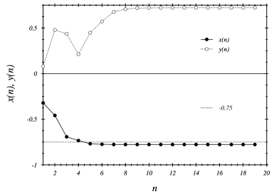
Figure 7: Quantities $x,y$ [cf. eqns. (LABEL:eq_x),(LABEL:eq_y)] for dimensions: $d_{0}=7$, $d_{1}=9$, $d_{2}=14$.

In Fig. 7 we have plotted the quantities $x$ and $y$ vs. $n$ which enter in (LABEL:eq_x) and (LABEL:eq_y).

The quantity $x^{(n)}$ appears to be rather stable around -0.75 for $n\geq 3$ and yields a value of $\nu_{1}=1$ for the critical exponent appearing in (101). The vanishing of the singlet-triplet gap (101) in the thermodynamical limit has been suggested by Tang and Hirsch (tang89, ) from a finite-size analysis of the ground state energies. On the other hand $y^{(n)}$ is not yet stable with respect to $n$. Again the reason might be that our truncation of the dimensions $d_{S}$ for the interaction matrices $\Delta_{S}$ $S=0,1,2,$ still needs to be improved.

VIII The staggered magnetization

The real space renormalization group approach generates a recursion formula for the singlet ground state $|\sigma^{(n+1)}\rangle$ (67) which enters in the definition of the staggered magnetization

$$\langle\sigma^{(n+1)}|\Sigma_{-}^{(n+1)}\Sigma_{+}^{(n+1)}|\sigma^{(n+1)}\rangle\,.$$ (107)

Here

$$\Sigma_{\pm}^{(n+1)} = \frac{1}{4^{n+1}}\sum_{x}(-)^{x}S_{+}(x)$$

$$= \frac{1}{4}\sum_{j=1}^{4}\Sigma_{\pm}^{(n)}(P_{j})$$

is the properly normalized staggered spin operator on a ($n+1$)-cluster, which can be decomposed into the corresponding quantities on the four neighbouring $n$-clusters $P_{j}$, $j=1,2,3,4$, as shown in Fig. 1. This leads to the following recursion formula for the ratio

$$R^{(n+1)} = \frac{\langle\sigma^{(n+1)}|\Sigma_{-}^{(n+1)}\Sigma_{+}^{(n+1)}|\sigma^{(n+1)}\rangle}{\langle\sigma^{(n)}|\Sigma_{-}^{(n)}\Sigma_{+}^{(n)}|\sigma^{(n)}\rangle}$$ (109)

$$= \sum_{i^{\prime},i=1}^{7}\sigma_{i^{\prime}}^{(n+1)}\sigma_{i}^{(n+1)}\Gamma_{i^{\prime},i}(\gamma^{(n)})$$

In the evaluation of (109) we can use the fact that the singlet basis states $|i,0\rangle$ (Table 2) are invariant under rotations of the four plaquettes $P_{1},P_{2},P_{3},P_{4}$. Therefore, we are left with the computation of the matrix elements

$$\langle i^{\prime},0;n+1|\Sigma_{-}^{(n)}(P_{j})\Sigma_{+}^{(n)}(P_{1})|i,0;n+1\rangle,\quad j=1,2,3$$

(110)

which proceeds in the following steps:

• The application of staggered spin operators $\Sigma_{+}^{(n)}(P_{1})$ onto the singlet states $|i,0;n+1\rangle$ leads to triplet states, which are not rotational invariant. A convenient set of triplet basis states is defined in Appendix C [(291)-(LABEL:S+7_0)] together with the decomposition of

  $$\Sigma_{+}^{(n+1)}(P_{1})|i,0;n+1\rangle$$ (111)

  into these basis states [(302)-(347)].

• By rotation of the 4 plaquettes

  $$P_{1}\rightarrow P_{2}\quad P_{2}\rightarrow P_{3}\quad P_{3}\rightarrow P_{4}\quad P_{4}\rightarrow P_{1}\quad$$ (112)

  we obtain from the decomposition of (111) the corresponding decompositions

  $$\Sigma_{+}(P_{2})|i,0;n+1\rangle \Sigma_{+}(P_{3})|i,0;n+1\rangle$$ (113)

  into the triplet states (302)-(347).

• The scalar products (110) turn out to be proportional to

  $$M^{(n)}(1,P,0)^{2}\quad M^{(n)}(1,P,0)M^{(n)}(2,P,1)$$

  $$M^{(n)}(2,P,1)^{2}$$ (114)

  where

  $$M^{(n)}(S+1,P,S) = \sum_{x\in P}(-)^{x}M^{(n)}(S+1,x,S)$$

  are just given by the reduced matrix elements (LABEL:wigner-eckart) summed over all sites of the $n$-cluster $P$.

  $$M^{(n)}(1,P,0)^{2} = \langle\sigma^{(n)}|\Sigma_{-}^{(n)}\Sigma_{+}^{(n)}|\sigma^{(n)}\rangle$$ (116)

  can be identified with the staggered magnetization on the $n$-cluster $P$, whereas the ratio

  $$\frac{M^{(n)}(2,P,1)}{M^{(n)}(1,P,0)} = \gamma^{(n)}$$ (117)

  is given by (42).

• The decomposition

  $$\langle i^{\prime},0;n+1|\Sigma_{-}^{(n)}(P_{j})\Sigma_{+}^{(n)}(P_{1})|i,0;n+1\rangle =$$

  $$\Gamma_{i^{\prime},i}^{(j,0)}M^{(n)}(1,P,0)^{2}+\Gamma_{i^{\prime},i}^{(j,2)}M^{(n)}(2,P,1)^{2}$$

  $$+\Gamma_{i^{\prime},i}^{(j,1)}M^{(n)}(1,P,0)M^{(n)}(2,P,1)$$ (118)

  illustrates, that the $n$-dependence - i.e. size dependence $2^{n+1}\times 2^{n+1}$ - only enters via the reduced matrix elements $M^{(n)}(1,P,0)$, $M^{(n)}(2,P,1)$, whereas the $7\times 7$ matrices

  $$\Gamma_{i^{\prime},i}^{(j,0)},\Gamma_{i^{\prime},i}^{(j,1)},\Gamma_{i^{\prime},i}^{(j,2)}, i,i^{\prime}=1,..,7,\quad j=1,2,3$$

  are independent of $n$. They are not affected by the renormalization group procedure and can be completely expressed in terms of scalar products formed from the triplet states (cf. Appendix C).

This leads to an explicit expression (LABEL:Gamma1)-(375) of the $7\times 7$ matrix $\Gamma_{i^{\prime},i}(\gamma^{(n)})$, which enters into the recursion formula (109). The numerical evaluation of (109) is presented in Fig. 8.

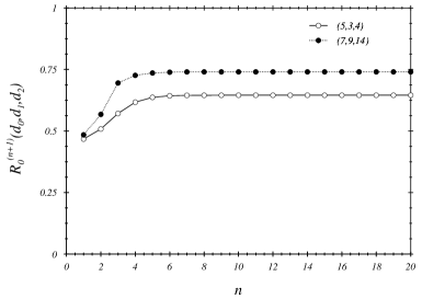
Figure 8: Evaluation of the recursion formula (109) for dimensions: $(d_{0},d_{1},d_{2})=$ $(5,3,4)$, $(7,9,14)$.

The ratio starts around $1/2$ and rapidly increases to $0.742$ and remains constant for $n\geq 4$. A nonvanishing staggered magnetization would demand a limiting value $R=1$ in the thermodynamical limit $n\rightarrow\infty$. The deviation from this value, we see in Fig. 8, has to be attributed to the truncation of the interaction matrices $\Delta_{S}$, $S=0,1,2$. Their dimensions $d_{S}$ are limited to

$$(d_{0},d_{1},d_{2}) = (7,9,14)$$ (120)

since we allow only for one quintuplet plaquette on the four cluster compound. We expect that the extension of the interaction matrices to four cluster states with $2,3,4$ quintuplets will lead to an increase of the ratio $R$. For the moment, we can only compare the difference of including one quintuplet (120) to zero quintuplet contributions:

$$(d_{0},d_{1},d_{2}) = (5,3,4)$$ (121)

The ratio $R$ is substantially lower in the case (121) as can be seen from Fig. 8.

In other words: Higher plaquette excitations are needed to generate plaquette-plaquette interactions which yield a nonvanishing staggered magnetization in the thermodynamical limit.

It has been observed already by Bernu et al. (bernu92, ) that the ground states in the total spin $S$ sectors collapse to the ground state in the thermodynamical limit.

IX Discussion and perspectives

If we compare our approach with previous renormalization group methods, we find on one hand the same goal - namely the derivation of a low energy effective Hamiltonian - but also crucial differences in the underlying assumptions:

Most of the “older” approaches like that of Lepetit and Manousakis (manousakis93, ) start with blocks with an odd number of sites. Here, the block ground state has spin $1/2$ and the Wigner-Eckart Theorem allows already interactions between neighbouring blocks in the ground state. Excited states - e.g. with total spin $3/2$ - are assumed to contribute only to a renormalization of the coupling between blocks in the ground state. Therefore, there is no renormalization of the energy difference between the ground state and excited states. In our opinion this is the reason, why these approaches do not allow for spin-spin correlations at large distances. The exact RG flow acts in an infinite-dimensional space of Hamiltonians resp. couplings. Even when starting with a model that is defined by very few couplings, the exact flow will carry the Hamiltonian into rather complicated regimes: at each step of an RG procedure longer-ranged couplings are generated. In the past, in many applications of the RG concept the space of all Hamiltonians was truncated to a finite dimensional one, i.e. only a few coupling constants were kept. For many universal properties, this approach was successful.

Recent approaches like ours and that of Capponi et al. (capponi04, ), Albuquerque et al. (troyer08, ) based on the CORE method (Contractor Renormalization group) (morningstar94, ) start with plaquettes having a singlet ground state. They cannot interact, since the interaction is mediated by the spin operators in the Hamiltonian. Their expectation values between total spin 0 states vanish according to the Wigner-Eckart Theorem. Therefore excited states on the plaquettes are absolutely necessary to generate interactions between the plaquettes [cf. the processes (38),(46),(47),(55),(62), (69),(77) of Section II]. For this reason we included triplet ($|A_{q}\rangle$, $q=\pm 1,0$) and quintuplet ($|Q_{r}\rangle$, $r=\pm 2,\pm 1,0$) excitations. Indeed it turned out that the states with one quintuplet excitation (i.e. $|6,0\rangle$ and $|7,0\rangle$ in Table 2 and $|k,+\rangle$, $k=4,5,..,9$ in Table 3 and $|3,2+\rangle$, $|6+j,2+\rangle$, $|9+j,2+\rangle$, $|12+j,2+\rangle$ ($j=0,1,2$) in Table 4) improve the decrease of the singlet-triplet gap in the large-$n$ limit

$$\rho^{*}(5,3,4)=-0.767 \rho^{*}(7,9,14)=-0.183$$ ; (122)

The limiting value (122) defines a measure for the “quality” of the singlet-triplet gap generated with interaction matrices $\Delta_{S}$ of dimensions $d_{S}$, $S=0,1,2$

$$(d_{0},d_{1},d_{2})=(5,\,3,\,4) (7,\,9,\,14)$$ ; (123)

Such an extension of the interaction matrices also leads to an improvement of the staggered magnetization, as discussed in Fig. 8.

In refs. (capponi04, ), (troyer08, ) the quintuplet excitations are missing and it would be interesting to see how the singlet-triplet gap decreases in their renormalization process. Note however, that quintuplet excitations possess large couplings (61) to triplet excitations, which do not die out in the renormalization process ($n\rightarrow\infty$) (Fig. 5); the corresponding energy differences (39), (40) decrease as well (Fig. 6). The authors of ref. (troyer08, ) intend to improve the CORE results by varying the compounds of plaquettes. In addition to the 4 plaquette compound of Fig. 1, they allow 2 and 3 plaquette compounds. We do not have this freedom, since our renormalization approach is restricted to the geometry of the 4 plaquette compound. The restriction to rotational symmetric states on the 4 plaquette compound with singlets, triplets and quintuplets enables us to follow the renormalization group flow for all couplings and gaps, which enter into the interaction matrices.

We intend to improve our results in a first step by taking into account all rotational symmetric states on the 4 plaquette compound with $n_{Q}=2,3,4$ quintuplets. Larger interaction matrices demand for an efficient method to calculate matrix elements which form $SU(2)$ invariants - similar to Racah coefficients (edmonds60, ) in Nuclear Physics.

Appendix A The interaction matrices

Here we present the interaction matrices $\Delta_{S}$, $S=0,1,2$. In order to clarify the dependence on the scaled energy gaps $\rho$, $\kappa$ and coupling constants $\gamma$, $\beta$, $\varepsilon$ [cf. eqs. (39)-(44)], it is convenient to consider the following block forms:

A.1 Spin 0 sector

$$\Delta_{0} = \left(\begin{array}[]{c|c}\Delta(5,5)&\Delta(5,6)\\ \Delta^{T}(5,6)&\Delta(6,6)\end{array}\right)$$ (126)

$\Delta(5,5)$ is fixed by the matrix elements of the first five states:

$$\Delta(5,5) = \left(\begin{array}[]{c|c|c|c|c}0&2\sqrt{3}&0&0&0\\ \hline\cr 2\sqrt{3}&2\rho-\beta&2\sqrt{2}&\frac{2}{\sqrt{3}}&2\sqrt{\frac{5}{3}}\\ \hline\cr 0&2\sqrt{2}&2\rho&0&0\\ \hline\cr 0&\frac{2}{\sqrt{3}}&0&4\rho&0\\ \hline\cr 0&2\sqrt{\frac{5}{3}}&0&0&4\rho+\frac{1}{2}\beta\end{array}\right)$$ (132)

Note that this block matrix only depends on $\rho$ and $\beta$.

The matrix elements between the states $i=1,\ldots,5$ and $i=6,7$ are contained in the $2\times 5$ block matrix

$$\Delta^{T}(5,6) = \gamma\left(\begin{array}[]{ccccc}0&0&2\sqrt{\frac{5}{3}}&\frac{2\sqrt{10}}{3}&\frac{\sqrt{2}}{3}\\ 0&2\sqrt{\frac{5}{3}}&0&0&0\end{array}\right)$$ (136)

which is proportional to $\gamma$.

The matrix elements $i=6,7$, $i^{\prime}=6,7$ form the third block matrix

$$\Delta(6,6) = (4\rho+\kappa)\mathbf{1}-\frac{1}{6}\beta\left(\begin{array}[]{cc}1&0\\ 0&0\end{array}\right)-\frac{\sqrt{3}}{2}\varepsilon\left(\begin{array}[]{cc}1&0\\ 0&2\end{array}\right)$$ (144)

$$+\Big{(}\sqrt{2}+\frac{1}{2\sqrt{3}}\gamma^{2}\Big{)}\left(\begin{array}[]{cc}0&1\\ 1&0\end{array}\right)$$

A.2 Spin 1 sector

$$\Delta_{1} = \left(\begin{array}[]{cc}\Delta(5,5)&\Delta(5,6)\\ \Delta^{T}(5,6)&\Delta(6,6)\end{array}\right)$$ (147)

$\Delta(5,5)$ is fixed by the matrix elements of the first five states:

$$\Delta(5,5)=$$

$$\left(\begin{array}[]{c|c|c||c|c}2&\frac{2}{\sqrt{3}}&2\sqrt{\frac{5}{3}}&-\gamma\sqrt{\frac{10}{3}}&0\\ \hline\cr\frac{2}{\sqrt{3}}&2\rho+\frac{2}{3}&\frac{2}{3}\sqrt{5}&-\frac{\sqrt{10}}{3}\gamma&-\frac{\sqrt{20}}{3}\gamma\\ \hline\cr 2\sqrt{\frac{5}{3}}&\frac{2}{3}\sqrt{5}&2\rho+\frac{1}{3}-\frac{3}{2}\beta&-\frac{1}{3\sqrt{2}}\gamma&-\frac{1}{3}\gamma\\ \hline\cr\hline\cr-\gamma\sqrt{\frac{10}{3}}&-\frac{\sqrt{10}}{3}\gamma&-\frac{1}{3\sqrt{2}}\gamma&\kappa+2\rho+&\sqrt{2}\\ &&&\frac{1}{6}\gamma^{2}-\frac{\sqrt{3}}{2}\varepsilon&\\ \hline\cr 0&-\frac{\sqrt{20}}{3}\gamma&-\frac{1}{3}\gamma&\sqrt{2}&\kappa+2\rho\end{array}\right)$$ (154)

The matrix elements between the states $k=1,\ldots,5$ and $k=6,7,8,9$ are contained in the $4\times 5$ block matrix

$$\Delta(5,6) = \left(\begin{array}[]{cccc}0&0&0&0\\[5.0pt] \frac{2\sqrt{5}}{3\sqrt{3}}\gamma&\frac{1}{3\sqrt{3}}\gamma&\frac{\sqrt{5}}{3}\gamma&\frac{2\sqrt{7}}{3}\gamma\\[5.0pt] \frac{1}{3\sqrt{3}}\gamma&\frac{23}{3\sqrt{15}}\gamma&-\frac{4}{3}\gamma&\frac{\sqrt{7}}{3\sqrt{5}}\gamma\\[5.0pt] -\frac{\sqrt{2}}{\sqrt{3}}&-\frac{\sqrt{10}}{\sqrt{3}}&0&0\\[5.0pt] 0&0&0&0\\ \end{array}\right)$$ (161)

The matrix elements $k=6,7,8,9$, $k^{\prime}=6,7,8,9$ form the third block matrix:

$$\Delta(6,6) = (4\rho+\kappa)\cdot\mathbf{1}+\frac{\beta}{2}\cdot\left(\begin{array}[]{cccc}0&0&0&0\\ 0&-3&0&0\\ 0&0&-1&0\\ 0&0&0&+2\end{array}\right)$$ (166)

$$+\varepsilon\cdot\left(\begin{array}[]{cccc}0&0&0&0\\ 0&-\frac{3\sqrt{3}}{4}&+\frac{3}{4\sqrt{5}}&0\\ 0&+\frac{3}{4\sqrt{5}}&-\frac{25\sqrt{3}}{36}&+\frac{7\sqrt{3}}{9\sqrt{35}}\\ 0&0&+\frac{7\sqrt{3}}{9\sqrt{35}}&-\frac{8\sqrt{3}}{9}\end{array}\right)$$ (172)

$$+\gamma^{2}\cdot\left(\begin{array}[]{cccc}\frac{10}{9}&\frac{\sqrt{5}}{90}&\frac{1}{6\sqrt{3}}&\frac{\sqrt{35}}{15\sqrt{3}}\\[5.0pt] \frac{\sqrt{5}}{90}&\frac{91}{180}&\frac{95\sqrt{3}}{180\sqrt{5}}&\frac{\sqrt{21}}{90}\\[5.0pt] \frac{1}{6\sqrt{3}}&\frac{95\sqrt{3}}{180\sqrt{5}}&-\frac{1}{12}&-\frac{\sqrt{7}}{6\sqrt{5}}\\[5.0pt] \frac{\sqrt{35}}{15\sqrt{3}}&\frac{\sqrt{21}}{90}&-\frac{\sqrt{7}}{6\sqrt{5}}&\frac{2}{15}\\ \end{array}\right)$$ (177)

A.3 Spin 2 sector

$$\Delta_{2} = \left(\begin{array}[]{c|ccc}\Delta(5,5)&\Delta(5,6)&\Delta(5,9)&\Delta(5,12)\\ \hline\cr\Delta^{T}(5,6)&\Delta(6,6)&\Delta(6,9)&\Delta(6,12)\\ \Delta^{T}(5,9)&\Delta^{T}(6,9)&\Delta(9,9)&0\\ \Delta^{T}(5,12)&\Delta^{T}(6,12)&0&\Delta(12,12)\end{array}\right)$$ (183)

$\Delta(5,5)$ is fixed by the matrix elements of the first five states:

$$\Delta(5,5) = \left(\begin{array}[]{c|c|c|c||c}+\frac{1}{2}\beta&2\sqrt{2}&\frac{2\sqrt{2}}{\sqrt{3}}&\frac{\sqrt{7}}{\sqrt{3}}&2\gamma\\ \hline\cr 2\sqrt{2}&0&0&0&0\\ \hline\cr\frac{2\sqrt{2}}{\sqrt{3}}&0&2\rho&0&0\\ \hline\cr\frac{\sqrt{7}}{\sqrt{3}}&0&0&2\rho+\frac{3}{7}\beta&0\\ \hline\cr\hline\cr 2\gamma&0&0&0&\kappa\end{array}\right)$$ (190)

$$\Delta(5,6) = \gamma\cdot\left(\begin{array}[]{c|c|c}-\frac{2}{\sqrt{3}}&0&-\frac{\sqrt{7}}{\sqrt{3}}\\ \hline\cr 0&0&0\\ \hline\cr 0&0&0\\ \hline\cr 0&0&0\\ \hline\cr 0&0&0\end{array}\right)$$ (197)

$$\Delta(5,9) = \left(\begin{array}[]{c|c|c}0&0&0\\ \hline\cr-\sqrt{\frac{2}{3}}\gamma&+\sqrt{\frac{3}{2}}\gamma&-\frac{\sqrt{7}}{\sqrt{6}}\gamma\\ \hline\cr-\frac{2\sqrt{2}}{3}\gamma&0&-\frac{\sqrt{2\cdot 7}}{3}\gamma\\ \hline\cr-\frac{\sqrt{7}}{3}\gamma&0&\frac{1}{3}\gamma\\ \hline\cr-\sqrt{3}&0&0\end{array}\right)$$ (203)

$$\Delta(5,12) = \left(\begin{array}[]{c|c|c}0&0&0\\ \hline\cr-\sqrt{\frac{2}{3}}\gamma&-\sqrt{\frac{3}{2}}\gamma&-\frac{\sqrt{7}}{\sqrt{6}}\gamma\\ \hline\cr-\frac{2\sqrt{2}}{3}\gamma&0&-\frac{\sqrt{2\cdot 7}}{3}\gamma\\ \hline\cr-\frac{\sqrt{7}}{3}\gamma&0&\frac{1}{3}\gamma\\ \hline\cr-\sqrt{3}&0&0\end{array}\right)$$ (209)

$$\Delta(6,6) = \Big{(}2\rho+\kappa\Big{)}\cdot\mathbf{1}+\varepsilon\Big{(}K+\tilde{K}\Big{)}$$ (210)

$$K = \frac{1}{4\sqrt{3}}\left(\begin{array}[]{ccc}0&4&0\\ 4&-1&\sqrt{7}\\ 0&\sqrt{7}&-3\end{array}\right)$$ (214)

$$\tilde{K} = FKF;\quad F=\left(\begin{array}[]{ccc}1&0&0\\ 0&-1&0\\ 0&0&1\end{array}\right)$$ (218)

$$\Delta(9,9) = \Big{(}2\rho+\kappa\Big{)}\cdot\mathbf{1}+\varepsilon\cdot K+\frac{\beta}{2}\left(\begin{array}[]{ccc}-2&0&0\\ 0&-1&0\\ 0&0&1\end{array}\right)$$ (222)

$$\Delta(12,12) = \Big{(}2\rho+\kappa\Big{)}\cdot\mathbf{1}+\varepsilon\cdot\tilde{K}+\frac{\beta}{2}\left(\begin{array}[]{ccc}-2&0&0\\ 0&-1&0\\ 0&0&1\end{array}\right)$$ (227)

$$\Delta(6,9) = F+\gamma^{2}C$$ (229)

$$\Delta(6,12) = F+\gamma^{2}FCF$$ (230)

$$C = \frac{1}{6}\left(\begin{array}[]{ccc}2&3&\sqrt{7}\\ 3&3&0\\ \sqrt{7}&0&-1\end{array}\right)$$ (234)

Appendix B Coefficients (71)-(74)

In this Appendix the coefficients (71)-(74) of Section V are given. Note that the dimensions $d_{S}=7,9,14$ have been used.

Note further, that those nonzero coefficients with spin 2 plaquette contribution are marked with boxes. I.e., the reduced Hilbert space [$(d_{0},d_{1},d_{2})=(5,3,4)$] for zero spin 2 plaquettes is directly illustrated.

$$I_{k,i} = \left(\begin{array}[]{ccccc|cc}-\frac{1}{2}&-\frac{1}{2\sqrt{3}}&-\frac{1}{2\sqrt{6}}&0&0&0&0\\ 0&-\frac{1}{6}&-\frac{1}{2\sqrt{2}}&-\frac{1}{2\sqrt{3}}&0&\framebox{$-\frac{5}{6\sqrt{30}}$}&0\\ 0&-\frac{\sqrt{5}}{6}&0&0&-\frac{7}{20\sqrt{3}}&\framebox{$-\frac{1}{12\sqrt{6}}$}&\framebox{$-\frac{1}{4\sqrt{3}}$}\\ \hline\cr 0&\framebox{$-\frac{\sqrt{5}}{6\sqrt{2}}$}&0&0&0&+\frac{1}{10\sqrt{3}}&+\frac{1}{5\sqrt{6}}\\ 0&0&\framebox{$+\frac{\sqrt{10}}{12}$}&0&0&+\frac{\sqrt{2}}{4\sqrt{3}}&0\\ 0&0&0&\framebox{$-\frac{16+\sqrt{6}}{35\sqrt{5}}$}&0&-\frac{1}{6\sqrt{2}}&0\\ 0&0&0&\framebox{$-\frac{22+\sqrt{6}}{360}$}&\framebox{$-\frac{45+\sqrt{2}}{60\sqrt{5}}$}&-\frac{1}{12\sqrt{10}}&-\frac{7+3\sqrt{2}}{40\sqrt{5}}\\ 0&0&0&\framebox{$-\frac{10\sqrt{3}-3\sqrt{2}}{72\sqrt{5}}$}&\framebox{$-\frac{\sqrt{3}}{60}$}&-\frac{1}{4\sqrt{6}}&+\frac{7\sqrt{3}+3\sqrt{6}}{120}\\ 0&0&0&\framebox{$-\frac{2\sqrt{3}+3\sqrt{2}}{90\sqrt{7}}$}&\framebox{$-\frac{2}{5\sqrt{105}}$}&-\frac{2}{\sqrt{210}}&-\frac{3+16\sqrt{2}}{10\sqrt{210}}\\ \end{array}\right)$$ (244)

$$G_{l,k} = \left(\begin{array}[]{ccc|cccccc}-\frac{1}{2}&-\frac{1}{2\sqrt{3}}&-\frac{1}{4\sqrt{15}}&\framebox{$+\frac{1}{4\sqrt{30}}$}&0&0&0&0&0\\ -\frac{1}{2\sqrt{2}}&0&-\frac{\sqrt{6}}{4\sqrt{5}}&0&\framebox{$+\frac{1}{4\sqrt{30}}$}&0&0&0&0\\ 0&-\frac{1}{2\sqrt{2}}&-\frac{1}{\sqrt{10}}&0&0&\framebox{$-\frac{1}{4\sqrt{30}}$}&\framebox{$-\frac{\sqrt{6}}{120}$}&\framebox{$-\frac{1+2\sqrt{2}}{4\sqrt{10}}$}&\framebox{$-\frac{\sqrt{7}}{10\sqrt{2}}$}\\ 0&+\frac{1}{4\sqrt{7}}&-\frac{1}{4\sqrt{5\cdot 7}}&0&0&\framebox{$+\frac{1}{12\sqrt{105}}$}&\framebox{$-\frac{2}{3\sqrt{21}}$}&\framebox{$+\frac{3\sqrt{5}}{12\sqrt{7}}$}&\framebox{$-\frac{1}{84}$}\\ \hline\cr\framebox{$-\frac{1}{4}$}&0&0&+\frac{\sqrt{6}}{4\sqrt{5}}&+\frac{\sqrt{3}}{4\sqrt{5}}&0&0&0&0\\ 0&\framebox{$+\frac{1}{4}$}&0&-\frac{1}{2\sqrt{10}}&0&+\frac{3}{2\sqrt{60}}&0&0&0\\ 0&0&0&0&0&0&0&0&0\\ 0&0&\framebox{$+\frac{\sqrt{7}}{8\sqrt{5}}$}&-\frac{\sqrt{7}}{4\sqrt{10}}&0&0&+\frac{11\sqrt{3}}{80\sqrt{7}}&+\frac{33}{48\sqrt{35}}&+\frac{11}{280}\\ 0&\framebox{$+\frac{1}{12}$}&\framebox{$+\frac{1}{6\sqrt{5}}$}&-\frac{1}{4\sqrt{10}}&-\frac{1}{4\sqrt{5}}&+\frac{1}{4\sqrt{15}}&+\frac{1}{4\sqrt{3}}&0&0\\ 0&\framebox{$+\frac{1}{8}$}&\framebox{$+\frac{1}{16\sqrt{5}}$}&-\frac{1}{8\sqrt{10}}&-\frac{3}{8\sqrt{5}}&+\frac{3}{8\sqrt{15}}&-\frac{\sqrt{3}}{16}&+\frac{3}{16\sqrt{5}}&0\\ 0&\framebox{$+\frac{\sqrt{7}}{24}$}&\framebox{$+\frac{\sqrt{7}}{48\sqrt{5}}$}&-\frac{\sqrt{7}}{8\sqrt{10}}&-\frac{\sqrt{7}}{8\sqrt{5}}&+\frac{\sqrt{7}}{8\sqrt{15}}&+\frac{19-12\sqrt{2}}{80\sqrt{21}}&-\frac{17+4\sqrt{2}}{48\sqrt{35}}&+\frac{17+4\sqrt{2}}{420}\\ 0&\framebox{$+\frac{1}{12}$}&\framebox{$+\frac{1}{6\sqrt{5}}$}&-\frac{1}{4\sqrt{10}}&-\frac{1}{4\sqrt{5}}&+\frac{1}{4\sqrt{15}}&+\frac{1}{4\sqrt{3}}&0&0\\ 0&\framebox{$-\frac{1}{8}$}&\framebox{$-\frac{1}{16\sqrt{5}}$}&+\frac{1}{8\sqrt{10}}&+\frac{3}{8\sqrt{5}}&-\frac{3}{8\sqrt{15}}&+\frac{\sqrt{3}}{16}&-\frac{3}{16\sqrt{5}}&0\\ 0&\framebox{$+\frac{\sqrt{7}}{24}$}&\framebox{$+\frac{\sqrt{7}}{48\sqrt{5}}$}&-\frac{\sqrt{7}}{8\sqrt{10}}&-\frac{\sqrt{7}}{8\sqrt{5}}&+\frac{\sqrt{7}}{8\sqrt{15}}&+\frac{19-12\sqrt{2}}{80\sqrt{21}}&-\frac{17+4\sqrt{2}}{48\sqrt{35}}&+\frac{17+4\sqrt{2}}{420}\\ \end{array}\right)$$ (260)

$$F_{\xi,\xi}: \begin{array}[]{c|cc}j&F_{j,j}&\framebox{$F_{j,j}$}\\ \hline\cr 1&\frac{1}{2\sqrt{2}}&-\\ 2&\frac{1}{2\sqrt{2}}&-\\ 3&\frac{1}{2\sqrt{2}}&-\\ 4&-\frac{\sqrt{2}}{28}&-\\ \hline\cr\hline\cr 5&-&\frac{1}{2\sqrt{6}}\\ 6&-&\frac{1}{2\sqrt{6}}\\ 7&\frac{1}{12\sqrt{2}}&\frac{5}{12\sqrt{6}}\\ 8&\frac{1}{4\sqrt{2}}&\frac{1}{4\sqrt{6}}\\ 9&-&\frac{1}{2\sqrt{6}}\\ 10&\frac{1}{12\sqrt{2}}&\frac{5}{12\sqrt{6}}\\ 11&\frac{1}{4\sqrt{2}}&\frac{1}{4\sqrt{6}}\\ 12&-&\frac{1}{2\sqrt{6}}\\ 13&\frac{1}{12\sqrt{2}}&\frac{5}{12\sqrt{6}}\\ 14&\frac{1}{4\sqrt{2}}&\frac{1}{4\sqrt{6}}\\ \end{array}$$ (277)

$$F_{\tau,\tau}: \begin{array}[]{c|cc}j&F_{j,j}&\framebox{$F_{j,j}$}\\ \hline\cr 1&\frac{1}{4\sqrt{2}}&-\\ 2&\frac{1}{4\sqrt{2}}&-\\ 3&\frac{7}{40\sqrt{2}}&-\\ \hline\cr\hline\cr 4&-\frac{1}{8\sqrt{2}}&\frac{3}{8\sqrt{6}}\\ 5&-\frac{1}{8\sqrt{2}}&\frac{3}{8\sqrt{6}}\\ 6&-\frac{11}{25}\cdot\frac{1}{4\sqrt{2}}&+\frac{3}{2}\cdot\frac{1}{4\sqrt{6}}\\ 7&-\frac{1}{2}\cdot\frac{1}{4\sqrt{2}}&+\frac{69}{50}\cdot\frac{1}{4\sqrt{6}}\\ 8&+\frac{1}{2}\cdot\frac{1}{4\sqrt{2}}&+\frac{1}{2}\cdot\frac{1}{4\sqrt{6}}\\ 9&+2\cdot\frac{1}{4\sqrt{2}}&-\frac{1}{4\sqrt{6}}\\ \end{array}$$ (289)

Appendix C Recursion formula for the staggered magnetization

As explained in Section VIII the derivation of (109) follows the steps

• The application of the staggered spin operator $\Sigma_{+}^{(n)}(P_{1})$ onto the singlet basis states $|i,0;n+1\rangle$ - listed in Table 2 - generate triplet states, which are not rotational invariant:

  $$\Sigma_{+}^{(n)}(P_{1})|1,0\rangle = -M^{(n)}(1,P,0)|A_{+},0,0,0\rangle$$ (291)

  $$\Sigma_{+}^{(n)}(P_{1})|2,0\rangle = -\frac{1}{\sqrt{12}}M^{(n)}(1,P,0)\times$$

  $$\Big{[}|0,0,0,A_{+}\rangle+|0,A_{+},0,0\rangle$$

  $$+|A_{+},A_{q},A_{-q},0\rangle+|A_{+},0,A_{q},A_{-q}\rangle\Big{]}$$

  $$-\frac{1}{\sqrt{12}}M^{(n)}(2,P,1)\times$$

  $$\Big{[}|Q_{1-q},0,0,A_{q}\rangle+|Q_{1-q},A_{q},0,0\rangle\Big{]}$$

  $$\Sigma_{+}^{(n)}(P_{1})|3,0\rangle = -\frac{1}{\sqrt{6}}M^{(n)}(1,P,0)\times$$

  $$\Big{[}|0,0,A_{+},0\rangle+|A_{+},A_{q},0,A_{-q}\rangle\Big{]}$$

  $$-\frac{1}{\sqrt{6}}M^{(n)}(2,P,1)|Q_{1-q},0,A_{q},0\rangle$$

  $$\Sigma_{+}^{(n)}(P_{1})|4,0\rangle = -\frac{1}{3}M^{(n)}(1,P,0)|0,A_{q},A_{+},A_{-q}\rangle$$

  $$-\frac{1}{3}M^{(n)}(2,P,1)|Q_{1-p},A_{q},A_{p},A_{-q}\rangle$$

  $$\Sigma_{+}^{(n)}(P_{1})|5^{\prime},0\rangle = -2M^{(n)}(1,P,0)\times$$

  $$\Big{[}|0,A_{q},A_{-q},A_{+}\rangle+|0,A_{+},A_{q},A_{-q}\rangle\Big{]}$$

  $$-2M^{(n)}(2,P,1)\times$$

  $$\Big{[}|Q_{1+q},A_{-p},A_{p},A_{-q}\rangle$$

  $$+|Q_{1+q},A_{-q},A_{-p},A_{p}\rangle\Big{]}$$

  $$\Sigma_{+}^{(n)}(P_{1})|6,0\rangle = -\frac{1}{2\sqrt{10}}M^{(n)}(1,P,0)\times$$

  $$\Big{[}|0,0,Q_{1-q},A_{q}\rangle+|0,A_{q},Q_{1-q},0\rangle$$

  $$+|0,A_{q},0,Q_{1-q}\rangle+|0,Q_{1-q},0,A_{q}\rangle$$

  $$+|A_{+},Q_{-r},A_{q},A_{p}\rangle+|A_{+},A_{r},A_{q},Q_{-r}\rangle\Big{]}$$

  $$-\frac{1}{2\sqrt{10}}M^{(n)}(2,P,1)\times$$

  $$\Big{[}-|A_{1-r},A_{q},A_{p},0\rangle_{2}-|A_{1-r},0,A_{p},A_{q}\rangle_{2}$$

  $$+|Q_{1+p},0,Q_{-r},A_{-q}\rangle+|Q_{1+q},A_{p},0,Q_{-r}\rangle$$

  $$+|Q_{1+p},A_{q},Q_{-r},0\rangle+|Q_{1+q},Q_{-r},0,A_{p}\rangle\Big{]}$$

  $$\Sigma_{+}^{(n)}(P_{1})|7,0\rangle = -\frac{1}{\sqrt{20}}M^{(n)}(1,P,0)\times$$

  $$\Big{[}|0,Q_{1-p},A_{p},0\rangle+|0,0,A_{q},Q_{1-q}\rangle$$

  $$+|A_{+},A_{q},Q_{-r},A_{p}\rangle\Big{]}$$

  $$-\frac{1}{\sqrt{20}}M^{(n)}(2,P,1)\times$$

  $$\Big{[}-|A_{1-p-q},A_{p},0,A_{q}\rangle_{2}$$

  $$+|Q_{1+q},Q_{-r},A_{p},0\rangle$$

  $$+|Q_{1+p},0,A_{q},Q_{-r}\rangle\Big{]}$$

  It is convenient to express these states in a new basis which defines the occupation of the plaquettes $P_{1}$ $P_{2}$ $P_{3}$ $P_{4}$ in cyclic order, e.g.

  $$\Sigma_{+}^{(n)}(P_{1})|1,0\rangle = -M^{(n)}(1,P,0)|A_{+},0,0,0\rangle$$ (298)

  where

  $$-M^{(n)}(1,P,0) = \langle A_{+},0,0,0|\Sigma_{+}(P_{1})|1,0\rangle$$ (299)

  $$|A_{+},0,0,0\rangle = \left(\begin{array}[]{cc}0&0\\ A_{+}&0\end{array}\right)$$ (302)

  In this way, we are led to the following triplet states:

  $$|A_{+},A_{q},A_{-q},0\rangle = \sum_{q}(-)^{q}\left(\begin{array}[]{cc}A_{q}&A_{-q}\\ A_{+}&0\end{array}\right)$$ (305)

  $$|Q_{1-q},0,0,A_{q}\rangle = \sum_{q}(-)^{q}\left(\begin{array}[]{cc}0&0\\ Q_{1-q}&A_{q}\end{array}\right)$$ (311)

  $$\hskip 11.38092pt\times\left(\begin{array}[]{c|cc}2&1&1\\ 1-q&1&-q\end{array}\right)$$

  $$|Q_{1-p},A_{q},A_{p},A_{-q}\rangle = \sum_{p,q}(-)^{p+q}\left(\begin{array}[]{cc}A_{q}&A_{p}\\ Q_{1-p}&A_{-q}\end{array}\right)$$ (317)

  $$\hskip 11.38092pt\times\left(\begin{array}[]{c|cc}2&1&1\\ 1-p&1&-p\end{array}\right)$$

  $$|A_{+},Q_{-r},A_{q},A_{p}\rangle = \sum_{p,q}(-)^{p+q}\left(\begin{array}[]{c|cc}2&1&1\\ r&q&p\end{array}\right)$$ (323)

  $$\hskip 11.38092pt\times\left(\begin{array}[]{cc}Q_{-r}&A_{q}\\ A_{+}&A_{p}\end{array}\right)$$

  $$|A_{1+p},0,Q_{-r},A_{q}\rangle=\sum_{p,q}(-)^{p+q}\times$$

  $$\left(\begin{array}[]{c|cc}2&1&1\\ r&p&q\end{array}\right)\left(\begin{array}[]{cc}0&Q_{-r}\\ A_{1+p}&A_{q}\end{array}\right)\left(\begin{array}[]{c|cc}2&1&1\\ 1+p&1&p\end{array}\right)$$ (330)

  $$|A_{1-r},A_{q},A_{p},0\rangle_{2}=\sum_{p,q}(-)^{p+q}\times$$ (338)

  $$\left(\begin{array}[]{c|cc}2&1&1\\ r&q&p\end{array}\right)\left(\begin{array}[]{c|cc}2&1&1\\ -r&-1&1-r\end{array}\right)\left(\begin{array}[]{cc}A_{q}&A_{p}\\ A_{1-r}&0\end{array}\right)$$

  (339)

  $$|Q_{1+p},0,Q_{-r},A_{q}\rangle=\sum_{p,q}(-)^{p+q}\times$$

  $$\left(\begin{array}[]{c|cc}2&1&1\\ r&q&p\end{array}\right)\left(\begin{array}[]{c|cc}2&1&1\\ 1+p&1&p\end{array}\right)\left(\begin{array}[]{cc}0&Q_{-r}\\ Q_{p+1}&A_{q}\end{array}\right)$$ (346)

  (347)

  The transition matrix elements induced by staggered spin operators $\Sigma_{+}^{(n)}(P_{1})$ are expressed by the reduced matrix elements $M^{(n)}(1,P,0)$ (299) and $M^{(n)}(2,P,1)$ and appropriate Clebsch-Gordan coefficients; the latter are absorbed in the definitions (302)-(347) of the triplet states. Apart from rotations, there are two different states (305), (339) with three triplets. They turn out to be orthogonal to each other:

  $$\langle A_{+},A_{q},A_{-q},0|A_{1-r},A_{q},A_{p},0\rangle =$$

  $$=\sum_{q}(-)^{q}\left(\begin{array}[]{c|cc}2&1&1\\ 0&q&-q\end{array}\right)\left(\begin{array}[]{c|cc}2&1&1\\ 0&-1&1\end{array}\right) = 0$$ (352)

• In this step we rotate the triplet states (291)-(LABEL:S+7_0) and (302)-(347) as described in (112). In this way we obtain the decompositions (113).

• In this step we compute the scalar products (118). The $n$-independent $7\times 7$ matrix (109) is given as

  $$\Gamma(\gamma) = \left(\begin{array}[]{cc}\Gamma(5,5)&\Gamma(5,6)\\ \Gamma^{T}(5,6)&\Gamma(6,6)\end{array}\right),\quad i,i^{\prime}=1,2,3,4,5$$ (356)

  with

  $$\Gamma(5,5) = \frac{1}{4}\left(\begin{array}[]{ccccc}1&\frac{1}{\sqrt{3}}&\frac{1}{\sqrt{6}}&0&0\\ \frac{1}{\sqrt{3}}&1+\frac{\tilde{Y}}{6}&\frac{\sqrt{2}}{3}&\frac{1}{3\sqrt{3}}&\frac{7+\frac{1}{3}}{\sqrt{60}}\\ \frac{1}{\sqrt{6}}&\frac{\sqrt{2}}{3}&\frac{4+\tilde{Y}}{6}&\frac{1}{\sqrt{6}}&\frac{1}{\sqrt{30}}\\ 0&\frac{1}{3\sqrt{3}}&\frac{1}{\sqrt{6}}&\frac{1+\tilde{Y}}{3}&2\frac{1+\tilde{Y}}{3\sqrt{20}}\\ 0&\frac{7+\frac{1}{3}}{\sqrt{60}}&\frac{1}{\sqrt{30}}&2\frac{1+\tilde{Y}}{3\sqrt{20}}&\frac{7}{5}(1+\tilde{Y})\end{array}\right),$$

  $$\hskip 28.45274pt\tilde{Y}=\gamma^{2}Y$$

  $$\Gamma^{T}(5,6) = \frac{\gamma}{4}\left(\begin{array}[]{ccccc}0&\frac{Y}{2\sqrt{30}}&\frac{Y}{2\sqrt{15}}&\frac{Y}{3\sqrt{10}}&\frac{1}{10\sqrt{2}}(1+\frac{4}{3}Y)\\ 0&\frac{Y}{2\sqrt{15}}&0&\frac{Y}{6\sqrt{5}}&\frac{1}{6}Y\\ \end{array}\right),$$ (367)

  $$\Gamma(6,6) = \frac{1}{80}\Bigg{[}\left(\begin{array}[]{cc}x_{1}&0\\ 0&x_{2}\end{array}\right)$$ (375)

  $$\hskip 14.22636pt+\sqrt{2}\Big{(}2Y+\gamma^{2}(X+Z)\Big{)}\left(\begin{array}[]{cc}0&1\\ 1&0\end{array}\right)\Bigg{]}\,.$$

  with:

  $$x_{1} = 3Y+10+\gamma^{2}(2Y+3Z)$$ (376)

  $$x_{2} = 2Y+5+\gamma^{2}(Y+2Z)$$ (378)

  $$X=\frac{16}{9},\,\,\,Y=\frac{5}{3},\,\,\,Z=\frac{41}{18}.$$

References

• (1) J.G. Bednorz, K.A. MΓΌller, Z. Phys. B 64, 189 (1986)
• (2) J. Hubbard, Proc. Roy. Soc. A 276, 238 (1963)
• (3) P.W. Anderson, Science 235, 1196 (1987)
• (4) G. Baskaran, Z. Zou, P.W. Anderson, Sol. State Comm. 63, 973 (1987)
• (5) H.J. Schulz, T.A.L. Ziman, Europhys. Lett. 18, 355 (1992)
• (6) E. Manousakis, Rev. Mod. Phys. 63, 1 (1991)
• (7) H.Q. Lin, D.K. Campbell, Phys. Rev. Lett. 69, 2415 (1992)
• (8) H.Q. Lin, D.K. Campbell, Y.C. Cheng, C.Y. Pan, Phys. Rev. B 50, 12702 (1994)
• (9) S. Chakravarty, B.I. Halperin, D.R. Nelson, Phys. Rev. Lett. 60, 1057 (1988); Phys. Rev. B 39 (1989)
• (10) D.S. Fisher, Phys. Rev. B 39, 11783 (1989)
• (11) I. Affleck, Phys. Rev. Lett. 56, 746 (1986)
• (12) I. Affleck, F.D.M. Haldane, Phys. Rev. B 36, 5291 (1987)
• (13) C. J. Hamer, W. Zheng, and J. Oitmaa, Phys. Rev. B 50, 6877 (1994)
• (14) D.A. Huse, Phys. Rev. B 37, 2380 (1988)
• (15) A. W. Sandvik, Phys. Rev. B 56, 11678 (1997)
• (16) U. LΓΆw, Phys. Rev. B 76, 220409 (2007)
• (17) A.R. Edmonds, β€œAngular Momentum in Quantum Mechanics”, Princeton University Press (1960)
• (18) S. Tang, J.E. Hirsch, Phys. Rev. B 39, 4548 (1989)
• (19) B. Bernu, C. Lhuillier, L. Pierre, Phys. Rev. Lett. 69, 2590 (1992)
• (20) M.-B. Lepetit, E. Manousakis, Phys. Rev. B 48, 1028 (1993)
• (21) S. Capponi, A. LΓ€uchli, M. Mambrini, Phys. Rev. B 70, 104424 (2004); S. Capponi, Theor. Chem. Acc. 116, 524 (2006)
• (22) A. F. Albuquerque, M. Troyer, J. Oitmaa, Phys. Rev. B 78, 132402 (2008)
• (23) C. J. Morningstar and M. Weinstein, Phys. Rev. Lett. 73, 1873 (1994); Phys. Rev. D 54, 4131 (1996)
• (24) A. Fledderjohann, A. KlΓΌmper, K.-H. MΓΌtter, subm. to Eur. Phys. J. B, 2008