Chiral odd GPDs in transverse and longitudinal impact parameter spaces

Abstract

We investigate the chiral odd generalized parton distributions (GPDs) for non-zero skewness $\zeta$ in transverse and longitudinal position spaces by taking Fourier transform with respect to the transverse and longitudinal momentum transfer respectively. We present overlap formulas for the chiral-odd GPDs in terms of light-front wave functions (LFWFs) of the proton both in the ERBL and DGLAP regions. We calculate them in a field theory inspired model of a relativistic spin $1/2$ composite state with the correct correlation between the different LFWFs in Fock space, namely that of the quantum fluctuations of an electron in a generalized form of QED. We show the spin-orbit correlation effect of the two-particle LFWF as well as the correlation between the constituent spin and the transverse spin of the target.

I Introduction

Generalized parton distributions (GPDs) give a unified picture of the nucleon, in the sense that $x$ moments of them give the form factors accessible in exclusive processes whereas in the forward limit they reduce to parton distributions, accessible in inclusive processes (see rev for example). At zero skewness $\zeta$, if one performs a Fourier transform (FT) of the GPDs with respect to (wrt) the momentum transfer in the transverse direction $\Delta_{\perp}$, one gets the so called impact parameter dependent parton distributions, which tell us how the partons of a given longitudinal momentum are distributed in transverse position (or impact parameter $b_{\perp}$) space. These obey certain positivity constraints and unlike the GPDs themselves, have probabilistic interpretation bur . As transverse boost on the light-front is a Galilean boost, there are no relativistic corrections. Impact parameter dependent pdfs are defined for nucleon states localized in the transverse position space at $R_{\perp}$. In order to avoid a singular normalization constant, one can take a wave packet state. A wave packet state which is transversely polarized is shifted sideways in the impact parameter space burchi . An interesting interpretation of Ji’s angular momentum sum rule ji is obtained in terms of the impact parameter dependent pdfs burchi . On the other hand, in hadron_optics , real and imaginary parts of the DVCS amplitudes are expressed in longitudinal position space by introducing a longitudinal impact parameter $\sigma$ conjugate to the skewness $\zeta$, and it was shown that the DVCS amplitude show certain diffraction pattern in the longitudinal position space. Since Lorentz boosts are kinematical in the front form, the correlation determined in the three-dimensional $b_{\perp},\sigma$ space is frame-independent. As GPDs depend on a sharp $x$, the Heisenberg uncertainty relation restricts the longitudinal position space interpretation of GPDs themselves. It has, however, been shown in wigner that one can define a quantum mechanical Wigner distribution for the relativistic quarks and gluons inside the proton. Integrating over $k^{-}$ and $k^{\perp}$, one obtains a four dimensional quantum distribution which is a function of ${\vec{r}}$ and $k^{+}$ where ${\vec{r}}$ is the quark position vector defined in the rest frame of the proton. These distributions are related to the FT of GPDs in the same frame. This gives a 3D position space picture of the GPDs and of the proton, within the limitations mentioned above.

At leading twist, there are three forward parton distributions (pdfs), namely, the unpolarized, helicity and transversity distributions. Similarly, three leading twist generalized quark distributions can be defined which in the forward limit, reduce to these three forward pdfs. The third one is chiral odd and is called the generalized transversity distribution $F_{T}$. This is defined as the off-forward matrix element of the bilocal tensor charge operator. It is parametrized in terms of four GPDs, namely $H_{T}$, $\tilde{H}_{T}$, $E_{T}$ and $\tilde{E}_{T}$ in the most general way markus ; chiral ; burchi . Unlike $E$, which gives a sideways shift in the unpolarized quark density in a transversely polarized nucleon, the chiral-odd GPDs affect the transversely polarized quark distribution both in unpolarized and in transversely polarized nucleon in various ways. A relation for the transverse total angular momentum of the quarks has been proposed in burchi , in analogy with Ji’s relation, which involves a combination of second moments of $H_{T},E_{T}$ and $\tilde{H}_{T}$ in the forward limit. $\tilde{E}_{T}$ does not contribute when skewness $\zeta=0$, as it is an odd function of $\zeta$. $H_{T}$ reduces to the transversity distribution in the forward limit when the momentum transfer is zero. Unlike the chiral even GPDs, information about which can be and has been obtained from deeply virtual Compton scattering and hard exclusive meson production, it is very difficult to measure the chiral odd GPDs. That is because, being chiral odd, they have to combine with another chiral odd object in the amplitude. In double , a proposal to measure $H_{T}$ has been given in photo or electroproduction of a longitudinally polarized vector meson $\rho^{0}$ via two gluon fusion; this meson is separated by a large rapidity gap from other transversely polarized $\rho^{+}$ and the scattered neutron. The scattering amplitude factorizes and involves $H_{T}(x,\zeta,0)$ at zero momentum transfer as well as the chiral odd light-cone distribution amplitude for the transversely polarized meson. In gary , the exclusive process $\gamma^{*}P\rightarrow\pi^{0}P$ has been suggested to measure the tensor charge. However, one has to look at the helicity flip part which is a higher twist contribution. There is also a prospect of gaining information about the Mellin moments of chiral odd GPDs from lattice QCD lattice . They have been investigated in several models, the first being the bag model scopetta , where only $H_{T}$ has been found to be non-zero. In barbara , they have been calculated in a constituent quark model, a model independent overlap in the DGLAP region is also given. $H_{T}(x,\zeta,0)$ is also modeled in the ERBL region $x<\zeta$ in double . The possibility of getting model independent relations between transverse momentum dependent parton distributions and impact parameter representation of GPDs at $\zeta=0$ has been investigated in metz , however it was concluded that such relations are model dependent. In a previous work we have investigated the chiral odd GPDs for a simple spin-$1/2$ composite particle for $\zeta=0$ in impact parameter space harleen .

In this work, we present overlap formulas for the chiral odd GPDs in the terms of the LFWFs both in the DGLAP ($n\rightarrow n$) and ERBL ( $n+1\rightarrow n-1$) regions. We investigate them in a simple model, namely for the quantum fluctuations of a lepton in QED at one-loop order drell , the same system which gives the Schwinger anomalous moment $\alpha/2\pi$. We generalize this analysis by assigning a mass $M$ to the external electrons and a different mass $m$ to the internal electron lines and a mass $\lambda$ to the internal photon lines with $M<m+\lambda$ for stability. In effect, we shall represent a spin-${1\over 2}$ system as a composite of a spin-${1\over 2}$ fermion and a spin-$1$ vector boson hadron_optics ; dis ; dip ; dip2 ; marc . This field theory inspired model has the correct correlation between the Fock components of the state as governed by the light-front eigenvalue equation, something that is extremely difficult to achieve in phenomenological models. Also, it gives an intuitive understanding of the spin and orbital angular momentum of a composite relativistic system orbit . GPDs in this model satisfy general properties like polynomiality and positivity. So it is interesting to investigate the properties of GPDs in this model. By taking Fourier transform (FT) with respect to $\Delta_{\perp}$, we express the GPDs in transverse position space and by taking a FT with respect to $\zeta$ we expressed them in longitudinal position space.

II Overlap Representation

The chiral odd GPDs are expressed as the off forward matrix element of the bilocal tensor charge operator on the light cone. These involve a helicity flip of the quark.

We use the parametrization of burchi for the chiral odd GPDs:

$$F^{T\lambda^{\prime},\lambda}_{j} = P^{+}\int{dz^{-}\over 2\pi}e^{iP^{+}z^{-}\over 2}\langle P^{\prime},\lambda^{\prime}\mid{\bar{\psi}}({-z^{-}\over 2})\sigma^{+j}\gamma_{5}\psi({z^{-}\over 2})\mid P,\lambda\rangle$$ (1)

$$=H_{T}(x,\zeta,t){\bar{u}}(P^{\prime})\sigma^{+j}\gamma_{5}u(P)+\tilde{H}_{T}(x,\zeta,t)\epsilon^{+j\alpha\beta}{\bar{u}}(P^{\prime}){\Delta_{\alpha}P_{\beta}\over M^{2}}u(P)$$

$$+E_{T}(x,\xi,t)\epsilon^{+j\alpha\beta}{\bar{u}}(P^{\prime}){\Delta_{\alpha}\gamma_{\beta}\over 2M}u(P)+\tilde{E}_{T}(x,\zeta,t)\epsilon^{+j\alpha\beta}{\bar{u}}(P^{\prime}){P_{\alpha}\gamma_{\beta}\over M}u(P).$$

We choose the frame where the initial and final momenta of the proton with mass $M$ are:

$$P = \left(P^{+},0_{\perp},{M^{2}\over P^{+}}\right),$$ (2)

$$P^{\prime} = \left((1-\zeta)P^{+},-\Delta_{\perp},{M^{2}+\Delta_{\perp}^{2}\over(1-\zeta)P^{+}}\right).$$ (3)

So, the momentum transfered from the target is

$$\Delta=P-P^{\prime}=\left(\zeta P^{+},\Delta_{\perp},{t+\Delta_{\perp}^{2}\over\zeta P^{+}}\right),$$ (4)

where $t=\Delta^{2}$. Following overlap we expand the proton state of momentum $P$ and helicity $\lambda$ in terms of multi-particle light-front wave functions:

$$\mid P,\lambda\rangle = \sum_{n}\prod_{i=1}^{n}{dx_{i}d^{2}k_{\perp i}\over\sqrt{x_{i}}16\pi^{3}}16\pi^{3}\delta(1-\sum_{i=1}^{n}x_{i})\delta^{2}(\sum_{i=1}^{n}k_{\perp i})$$ (5)

$$~{}~{}\psi_{n}(x_{i},k_{\perp i},\lambda_{i})\mid n,x_{i}P^{+},x_{i}P_{\perp}+k_{\perp i},\lambda_{i}\rangle;$$

here $x_{i}=k_{i}^{+}/P^{+}$ is the light cone momentum fraction and $k_{\perp i}$ represent the relative transverse momentum of the $i$ th constituent. The physical transverse momenta are $p_{\perp i}=x_{i}P_{\perp}+k_{\perp i}$. $\lambda_{i}$ are the light-cone helicities. The light front wave functions $\psi_{n}$ are independent of $P^{+}$ and $P_{\perp}$ and are boost invariant.

Like the chiral even GPDs, here too there are diagonal $n\to n$ overlaps in the kinematical region $\zeta<x<1$ and $\zeta-1<x<0$. In the region $0<x<\zeta$ there are off diagonal $n+1\to n-1$ overlaps. The overlap representation of the chiral odd GPDs in terms of light front wave functions is given by :

$$F_{1,n\rightarrow n}^{T\lambda^{\prime},\lambda} = (1-\zeta)^{1-{n\over 2}}\sum_{n,\lambda_{i}}\int\Pi_{i=1}^{n}{dx_{i}d^{2}k_{\perp}^{i}\over 16\pi^{3}}16\pi^{3}\delta(1-\sum_{j}x_{j})\delta^{2}(\sum_{j=1}^{n}k_{\perp}^{j})\delta(x-x_{1})$$ (6)

$$\psi_{n}^{\lambda^{\prime}*}(x_{i}^{\prime},{k^{\prime}}_{\perp}^{i},\lambda^{\prime}_{i})\psi_{n}^{\lambda}(x_{i},k_{\perp}^{i},\lambda_{i})\delta_{\lambda_{1}^{\prime},-\lambda_{1}}[\delta_{\lambda_{i}^{\prime},\lambda_{i}}(i=2,..n)];$$

where ${x^{\prime}}_{i}={x_{i}\over 1-\zeta};~{}{k^{\prime}}_{\perp}^{i}=k_{\perp}^{i}+{x_{i}\over 1-\zeta}\Delta_{\perp}$ for $i=2,....n$ and ${x^{\prime}}_{1}={x_{1}-\zeta\over 1-\zeta};~{}{k^{\prime}}_{\perp}^{1}=k_{\perp}^{1}-{1-x_{1}\over 1-\zeta}\Delta_{\perp}$.

$$F_{1,n+1\rightarrow n-1}^{T\lambda^{\prime},\lambda} = {(1-\zeta)}^{3/2-n/2}\sum_{n,\lambda_{i}}\int\Pi_{i=1}^{n+1}{dx_{i}d^{2}k_{\perp}^{i}\over 16\pi^{3}}(16\pi^{3})^{2}\delta(1-\sum_{j=1}^{n+1}x_{j})\delta^{2}(\sum_{j=1}^{n+1}k_{\perp}^{i})\delta(x_{n+1}+x_{1}-\zeta)$$ (7)

$$\delta^{2}(k_{\perp n+1}+k_{1\perp}-\Delta_{\perp})\delta(x-x_{1})\psi_{n-1}^{\lambda^{\prime}*}(x_{i}^{\prime},{k^{\prime}}_{\perp}^{i},\lambda^{\prime}_{i})\psi_{n+1}^{\lambda}(x_{i},k_{\perp}^{i},\lambda_{i})$$

$$~{}~{}~{}~{}~{}~{}~{}~{}~{}~{}~{}~{}~{}~{}~{}~{}\delta_{\lambda_{1}^{\prime},-\lambda_{n+1}}[\delta_{\lambda_{i}^{\prime},\lambda_{i}}(i=2,..n)].$$

where ${x^{\prime}}_{i}={x_{i}\over 1-\zeta},~{}~{}~{}~{}~{}~{}~{}{k^{\prime}}_{\perp}^{i}=k_{\perp}^{i}+{x_{i}\over 1-\zeta}\Delta_{\perp}$, for $i=2,...n$ label the $n-1$ spectators. The overlaps are different from the chiral even GPDs as there is a helicity flip of the quark. The above overlap formulas can be used in any model calculation of the chiral odd GPDs using LFWFs.

III Chiral Odd GPDs in QED at One Loop

Following drell ; hadron_optics , we take a simple composite spin $1/2$ state, namely an electron in QED at one loop to investigate the GPDs. The light-front Fock state wavefunctions corresponding to the quantum fluctuations of a physical electron can be systematically evaluated in QED perturbation theory. The state is expanded in Fock space and there are contributions from $|\,{e^{-}\gamma}\rangle$ and $|\,{e^{-}e^{-}e^{+}}\rangle$, in addition to renormalizing the one-electron state. The two-particle state is expanded as,

$$\left|\Psi^{\uparrow}_{\rm two\ particle}(P^{+},\vec{P}_{\perp}=\vec{0}_{\perp})\right>=\int\frac{{\mathrm{d}}x\,{\mathrm{d}}^{2}{\vec{k}}_{\perp}}{\sqrt{x(1-x)}\,16\pi^{3}}$$

$$\left[\ \ \,\psi^{\uparrow}_{+\frac{1}{2}\,+1}(x,{\vec{k}}_{\perp})\,\left|+\frac{1}{2}\,+1\,;\,\,xP^{+}\,,\,\,{\vec{k}}_{\perp}\right>+\psi^{\uparrow}_{+\frac{1}{2}\,-1}(x,{\vec{k}}_{\perp})\,\left|+\frac{1}{2}\,-1\,;\,\,xP^{+}\,,\,\,{\vec{k}}_{\perp}\right>\right.$$

$$\left.{}\psi^{\uparrow}_{+\frac{1}{2}\,+1}(x,{\vec{k}}_{\perp})\,\left|+\frac{1}{2}\,+1\,;\,\,xP^{+}\,,\,\,{\vec{k}}_{\perp}\right>+\psi^{\uparrow}_{+\frac{1}{2}\,-1}(x,{\vec{k}}_{\perp})\,\left|+\frac{1}{2}\,-1\,;\,\,xP^{+}\,,\,\,{\vec{k}}_{\perp}\right>\right.$$

$$\left.{}+\psi^{\uparrow}_{-\frac{1}{2}\,+1}(x,{\vec{k}}_{\perp})\,\left|-\frac{1}{2}\,+1\,;\,\,xP^{+}\,,\,\,{\vec{k}}_{\perp}\right>+\psi^{\uparrow}_{-\frac{1}{2}\,-1}(x,{\vec{k}}_{\perp})\,\left|-\frac{1}{2}\,-1\,;\,\,xP^{+}\,,\,\,{\vec{k}}_{\perp}\right>\ \right]\ ,$$

where the two-particle states $|s_{\rm f}^{z},s_{\rm b}^{z};\ x,{\vec{k}}_{\perp}\rangle$ are normalized as in overlap . $s_{\rm f}^{z}$ and $s_{\rm b}^{z}$ denote the $z$-component of the spins of the constituent fermion and boson, respectively, and the variables $x$ and ${\vec{k}}_{\perp}$ refer to the momentum of the fermion. The light cone momentum fraction $x_{i}={k_{i}^{+}\over P^{+}}$ satisfy $0<x_{i}\leq 1$ and $\sum_{i}x_{i}=1$. We employ the light-cone gauge $A^{+}=0$, so that the gauge boson polarizations are physical. The three-particle state has a similar expansion. Both the two- and three-particle Fock state components are given in overlap . We here give the two-particle wave function for spin-up electron orbit ; drell ; overlap

$$\left\{\begin{array}[]{l}\psi^{\uparrow}_{+\frac{1}{2}\,+1}(x,{\vec{k}}_{\perp})=-{\sqrt{2}}\ \frac{-k^{1}+{i}k^{2}}{x(1-x)}\,\varphi\ ,\\ \psi^{\uparrow}_{+\frac{1}{2}\,-1}(x,{\vec{k}}_{\perp})=-{\sqrt{2}}\ \frac{k^{1}+{i}k^{2}}{1-x}\,\varphi\ ,\\ \psi^{\uparrow}_{-\frac{1}{2}\,+1}(x,{\vec{k}}_{\perp})=-{\sqrt{2}}\ (M-{m\over x})\,\varphi\ ,\\ \psi^{\uparrow}_{-\frac{1}{2}\,-1}(x,{\vec{k}}_{\perp})=0\ ,\end{array}\right.$$ (9)

$$\varphi(x,{\vec{k}}_{\perp})=\frac{e}{\sqrt{1-x}}\ \frac{1}{M^{2}-{{\vec{k}}_{\perp}^{2}+m^{2}\over x}-{{\vec{k}}_{\perp}^{2}+\lambda^{2}\over 1-x}}\ .$$ (10)

Similarly, the wave function for an electron with negative helicity can also be obtained.

Following the same references, we work in a generalized form of QED by assigning a mass $M$ to the external electrons and a different mass $m$ to the internal electron lines and a mass $\lambda$ to the internal photon lines. The idea behind this is to model the structure of a composite fermion state with mass $M$ by a fermion and a vector “diquark” constituent with respective masses $m$ and $\lambda$. The electron in QED also has a one-particle component

$$\left|\Psi_{\rm one\ particle}^{\uparrow,\downarrow}(P^{+},\vec{P}_{\perp}=\vec{0}_{\perp})\right>=\int{{\mathrm{d}}x\,{\mathrm{d}}^{2}{\vec{k}}_{\perp}\over\sqrt{x}\,16\pi^{3}}\ 16\pi^{3}\delta(1-x)\,{\delta}^{2}({\vec{k}}_{\perp})\ \psi_{(1)}\ \left|\pm{1\over 2}\,;xP^{+},{\vec{k}}_{\perp}\right>$$ (11)

where the one-constituent wavefunction is given by

$$\psi_{(1)}=\sqrt{Z}.$$ (12)

Here $\sqrt{Z}$ is the wavefunction renormalization of the one-particle state and ensures overall probability conservation. Also, in order to regulate the ultraviolet divergences we use a cutoff on the transverse momentum $k^{\perp}$. If, instead of imposing a cutoff on transverse momentum, we imposed a cutoff on the invariant mass orbit , then the divergences at $x=1$ would have been regulated by the non-zero photon mass.

In the domain $\zeta<x<1$, there are diagonal $2\to 2$ overlaps. These correspond to (setting $j=1$ in Eqn.(1)) the helicity non-flip $F_{1}^{T\uparrow\uparrow},F_{1}^{T\downarrow\downarrow}$ and helicity flip contributions, $F_{1}^{T\uparrow\downarrow},F_{1}^{T\downarrow\uparrow}$, respectively, which can be written as,

$$F_{1}^{T\uparrow\uparrow}=\int{d^{2}k_{\perp}\over 16\pi^{3}}\Big{[}\psi^{*1/2}_{1/2+1}(x^{\prime},k^{\prime}_{\perp})\psi^{1/2}_{-1/2+1}(x,k_{\perp})+\psi^{*1/2}_{-1/2+1}(x^{\prime},k^{\prime}_{\perp})\psi^{1/2}_{1/2+1}(x,k_{\perp})\Big{]};$$ (13)

$$F_{1}^{T\uparrow\downarrow}=\int{d^{2}k_{\perp}\over 16\pi^{3}}\Big{[}\psi^{*1/2}_{1/2+1}(x^{\prime},k^{\prime}_{\perp})\psi^{-1/2}_{-1/2+1}(x,k_{\perp})+\psi^{*1/2}_{1/2-1}(x^{\prime},k^{\prime}_{\perp})\psi^{-1/2}_{-1/2-1}(x,k_{\perp})\Big{]};$$ (14)

$$F_{1}^{T\downarrow\downarrow}=\int{d^{2}k_{\perp}\over 16\pi^{3}}\Big{[}\psi^{*-1/2}_{1/2-1}(x^{\prime},k^{\prime}_{\perp})\psi^{-1/2}_{-1/2-1}(x,k_{\perp})+\psi^{*-1/2}_{-1/2-1}(x^{\prime},k^{\prime}_{\perp})\psi^{-1/2}_{1/2-1}(x,k_{\perp})\Big{]};$$ (15)

$$F_{1}^{T\downarrow\uparrow}=\int{d^{2}k_{\perp}\over 16\pi^{3}}\Big{[}\psi^{*-1/2}_{-1/2-1}(x^{\prime},k^{\prime}_{\perp})\psi^{1/2}_{1/2-1}(x,k_{\perp})+\psi^{*-1/2}_{-1/2+1}(x^{\prime},k^{\prime}_{\perp})\psi^{1/2}_{1/2+1}(x,k_{\perp})\Big{]};$$ (16)

where

$$x^{\prime}={x-\zeta\over 1-\zeta},~{}~{}~{}~{}~{}~{}~{}~{}~{}~{}~{}~{}~{}~{}~{}~{}~{}k^{\prime}_{\perp}=k_{\perp}-(1-x^{\prime})\Delta_{\perp}.$$ (17)

$F_{1}^{T\uparrow\downarrow}$ and $F_{1}^{T\downarrow\uparrow}$ receive contribution from the single particle sector of the Fock space, which is strictly at $x=1$ (wavefunction renormalization) dip2 . We exclude $x=1$ by imposing a cutoff, and we do not consider this contribution in this work. It contributes also in the $3\to 1$ overlap, in the ERBL region. However, the single particle contribution is important as it cancels the singularity as $x\rightarrow 1$. This has been shown explicitly in the forward limit in tran , namely for the transversity distribution $h_{1}(x)$. The coefficient of the logarithmic term in the expression of $h_{1}(x)$ gives the correct splitting function for leading order evolution of $h_{1}(x)$; the delta function from the single particle sector providing the necessary ’plus’ prescription. In the off forward case, the cancellation occurs similarly, as shown for $F(x,\xi,t)$ in marc . The behavior at $x=0,1$ can be improved by differentiating the LFWFs with respect to $M^{2}$ har . The $x\to 0$ limit can be improved as well by a different method rad .

The GPDs are zero in the domain $\zeta-1<x<0$, which corresponds to emission and reabsorption of an $e^{+}$ from a physical electron. Contributions to the GPDs in that domain only appear beyond one-loop level.

In our model $F_{1}^{T\uparrow\downarrow}=F_{1}^{T\downarrow\uparrow}$ and thus

$${F_{1}^{T\uparrow\downarrow}-F_{1}^{T\downarrow\uparrow}\over 2} = \tilde{H}_{T}{1\over\sqrt{1-\zeta}}{\Delta^{1}\Delta^{2}\over M^{2}}$$ (18)

$$= 0.$$

Since the above equation is true for arbitrary $\Delta_{1},~{}\Delta_{2}$, it implies $\tilde{H}_{T}=0$ in our model. We define the combinations :

$$(-i\Delta_{2})A_{1} = {F_{1}^{T\uparrow\uparrow}+F_{1}^{T\downarrow\downarrow}\over 2}$$ (19)

$$= {-i\Delta_{2}\over 2M\sqrt{1-\zeta}}\Big{[}(2-\zeta)E_{T}+2\tilde{E}_{T}\Big{]};$$

$$(\Delta_{1})A_{2} = {F_{1}^{T\uparrow\uparrow}-F_{1}^{T\downarrow\downarrow}\over 2}$$ (20)

$$= {\Delta_{1}\over 2M\sqrt{-\zeta}}\Big{[}\zeta E_{T}+2\tilde{E}_{T}\Big{]};$$

$$iA_{3} = {F_{1}^{T\uparrow\downarrow}+F_{1}^{T\downarrow\uparrow}\over 2}$$ (21)

$$= i\Big{[}2H_{T}\sqrt{1-\zeta}-{\zeta^{2}\over 2\sqrt{1-\zeta}}E_{T}-{\zeta\over\sqrt{1-\zeta}}\tilde{E}_{T}\Big{]}.$$

From the above equations we have

$$E_{T}(x,\zeta,t) = {M\over\sqrt{1-\zeta}}(A_{1}-A_{2}),$$ (22)

$$\tilde{E}_{T}(x,\zeta,t) = {M\over 2\sqrt{1-\zeta}}\{(2-\zeta)A_{2}-\zeta A_{1}\},$$ (23)

$$H_{T}(x,\zeta,t) = {1\over 2\sqrt{1-\zeta}}(A_{3}+\zeta MA_{2}).$$ (24)

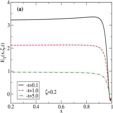
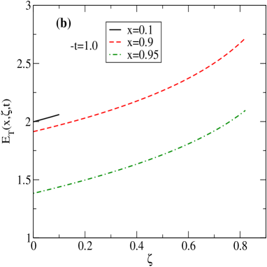
Figure 1: (Color online) Plot of $E_{T}(x,\zeta,t)$ (a) vs. $x$ for a fixed value of $\zeta=0.2$ and different values of $t$ in ${\mathrm{MeV}}^{2}$; (b) vs. $\zeta$ for different values of $x$ and for fixed $-t=1~{}{\mathrm{MeV}}^{2}$

Explicit matrix element calculation using Eqns(13-16) in our model gives

$$A_{1} = {\pi e^{2}\over 8\pi^{3}\sqrt{1-\zeta}}\Big{[}\{(M-{m\over x})x(1-\zeta)$$ (25)

$$~{}~{}~{}~{}~{}~{}~{}~{}~{}~{}~{}-(M-{m\over x^{\prime}})x^{\prime}\}(1-x^{\prime})I_{1}-(M-{m\over x})x(1-x)I_{2}\Big{]},$$

$$A_{2} = {\pi e^{2}\over 8\pi^{3}\sqrt{1-\zeta}}\Big{\{}(M-{m\over x})(1-x)xI_{2}-\Big{[}(M-{m\over x})(1-\zeta)x$$ (26)

$$~{}~{}~{}~{}~{}~{}~{}~{}~{}~{}~{}~{}~{}+(M-{m\over x^{\prime}})x^{\prime}\Big{]}(1-x^{\prime})I_{1}\Big{\}},$$

$$A_{3} = {e^{2}\over 16\pi^{3}}{(x+x^{\prime})\over\sqrt{(1-x)(1-x^{\prime})}}\Big{[}-I_{3}-I_{4}+B(x,\zeta)\pi I_{2}\Big{]};$$ (27)

here $B(x,\zeta)=M^{2}x^{\prime}(1-x^{\prime})-m^{2}(1-x^{\prime})-\lambda^{2}x^{\prime}+M^{2}x(1-x)-m^{2}(1-x)-\lambda^{2}x-(1-x^{\prime})^{2}\Delta_{\perp}^{2}$.

$$I_{1} = \int_{0}^{1}dy{1-y\over Q(y)},$$ (28)

$$I_{2} = \int_{0}^{1}dy{1\over Q(y)};$$ (29)

where $Q(y)=y(1-y)(1-x^{\prime})^{2}\Delta_{\perp}^{2}-y(M^{2}x(1-x)-m^{2}(1-x)-\lambda^{2}x)-(1-y)(M^{2}x^{\prime}(1-x^{\prime})-m^{2}(1-x^{\prime})-\lambda^{2}x^{\prime})$ and

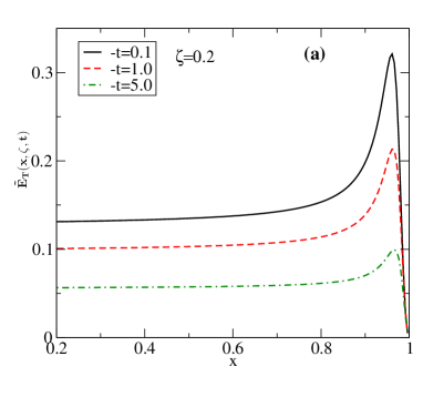
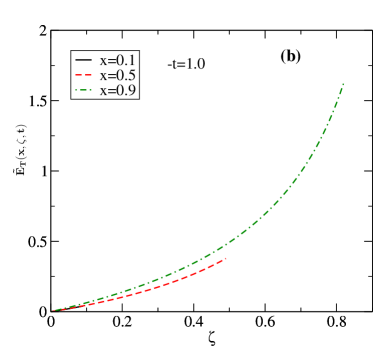
Figure 2: (Color online) Plot of $\tilde{E}_{T}(x,\zeta,t)$ (a) vs. $x$ for a fixed value of $\zeta=0.2$ and different values of $t$ in ${\mathrm{MeV}}^{2}$; (b) vs. $\zeta$ for different values of $x$ and for fixed $-t=1~{}{\mathrm{MeV}}^{2}$

$$I_{3} = \int_{0}^{\Lambda}d^{2}k_{\perp}{1\over-k_{\perp}^{2}+M^{2}x(1-x)-m^{2}(1-x)-\lambda^{2}x}$$ (30)

$$= -\pi\ln\mid{\Lambda^{2}\over m^{2}(1-x)+\lambda^{2}x-M^{2}x(1-x)}\mid;$$

$$I_{4} = \int_{0}^{\Lambda}d^{2}k_{\perp}{1\over-{k^{\prime}_{\perp}}^{2}+M^{2}x^{\prime}(1-x^{\prime})-m^{2}(1-x^{\prime})-\lambda^{2}x^{\prime}}$$ (31)

$$= -\pi\ln\mid{\Lambda^{2}\over m^{2}(1-x^{\prime})+\lambda^{2}x^{\prime}-M^{2}x^{\prime}(1-x^{\prime})}\mid.$$

So, we have the expressions for the GPDs

$$E_{T}(x,\zeta,t) = -{e^{2}\over 8\pi^{3}}{2M\pi\over 1-\zeta}(M-{m\over x})x(1-x)I_{5},$$ (32)

$$\tilde{E}_{T}(x,\zeta,t) = {e^{2}\over 8\pi^{3}}{M\pi\over 1-\zeta}\Big{[}-(1-x)\Big{\{}(M-{m\over x})x+(M-{m\over x^{\prime}})x^{\prime}\Big{\}}I_{1}$$ (33)

$$~{}~{}~{}~{}~{}~{}~{}~{}~{}+(M-{m\over x})x(1-x)I_{2}\Big{]},$$

$$H_{T}(x,\zeta,t) = {e^{2}\over 8\pi^{3}}{\pi\over 2}\Big{[}{x+x^{\prime}\over 2(1-x)}\ln({\Lambda^{4}\over DD^{\prime}})+\Big{\{}{x+x^{\prime}\over 2(1-x)}B(x,\zeta)+{\zeta M\over 1-\zeta}(M-{m\over x})x(1-x)\Big{\}}I_{2}$$ (34)

$$-{\zeta M\over 1-\zeta}\Big{\{}(M-{m\over x})x(1-\zeta)+(M-{m\over x^{\prime}})x^{\prime}\Big{\}}(1-x^{\prime})I_{1}\Big{]},$$

with

$$I_{5}=\int_{0}^{1}dy{y\over Q(y)},$$

$D=M^{2}x(1-x)-m^{2}(1-x)-\lambda^{2}x$ and $D^{\prime}=M^{2}x^{\prime}(1-x^{\prime})-m^{2}(1-x^{\prime})-\lambda^{2}x^{\prime}$.

All the numerical plots are performed in units of ${e^{2}/(8\pi^{3})}$. We took $M=0.51$  MeV, $m=0.5$  MeV and $\lambda=0.02$  MeV. In Figs. 1-3 (a), we have plotted the GPDs $E_{T},~{}\tilde{E}_{T}$ and $H_{T},$ as functions of x for fixed values of $\zeta=0.2$ and a fixed value of $t$. $H_{T}$ has logarithmic divergence, similar to the transversity distribution tran . For numerical analysis, we have used a cutoff $\Lambda=10$ MeV ($\Lambda>>M$) on transverse momentum. In Fig.(4), we show the cutoff dependence of $H_{T}$. However, one has to incorporate the single particle contribution to get the correct $+$ distribution and also to get a finite answer at $x=1$, as stated above. Both $E_{T}$ and $\tilde{E}_{T}$ are independent of $x$ at small and medium $x$ and at $x\to 1$, they are independent of $t$ bur and approach zero. Note that our analytic expressions for $H_{T}$ and $E_{T}$ agree with the quark model calculation of metz without the color factors, in the limit $\zeta=0$ and $M=m$ and $\lambda=0$. Fig. 1-3 (b) present the $\zeta$ behaviour of the above GPDs for fixed $t=-1.0~{}{\mathrm{MeV}}^{2}$ and different values of $x$. Note that as we are plotting in the DGLAP region, $x>\zeta$. Both $E_{T}$ and $\tilde{E}_{T}$ increases in magnitude with increase of $\zeta$ but $H_{T}$ decreases. $\tilde{E}_{T}$ is zero at $\zeta=0$.

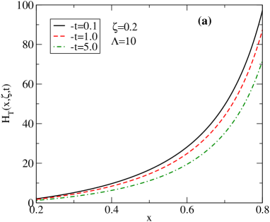
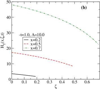
Figure 3: (Color online) Plot of $H_{T}(x,\zeta,t)$ (a) vs. $x$ for a fixed value of $\zeta=0.2$ and different values of $t$ in ${\mathrm{MeV}}^{2}$; (b) vs. $\zeta$ for different values of $x$ and for fixed $-t=1~{}{\mathrm{MeV}}^{2}$. $\Lambda$ is in MeV.

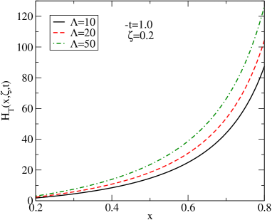
Figure 4: (Color online) $H_{T}(x,\zeta,t)$ for different UV cutoff $\Lambda$ (in MeV).

IV GPDs in position space

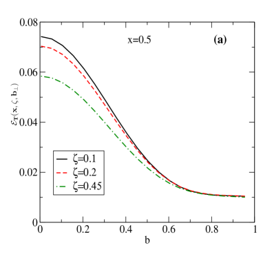
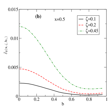
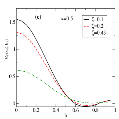
Figure 5: (Color online) Fourier spectrum of the chiral-odd GPDs vs. $\mid b_{\perp}\mid$ for fixed $x=0.5$ and different values of $\zeta$

Introducing the Fourier conjugate $b_{\perp}$ (impact parameter) of the transverse momentum transfer $\Delta_{\perp}$, the GPDs can be expressed in impact parameter space. Like the chiral even counterparts, chiral odd GPDs as well have interesting interpretation in impact parameter space. The second moment of $H_{T},E_{T}$ and ${\tilde{H}}_{T}$ is related to the transverse component of the total angular momentum carried by transversely polarized quarks in an unpolarized proton :

$$<J^{i}>={s^{i}\over 4}\int dxx\Big{[}H_{T}(x,0,0)+2\tilde{H}_{T}(x,0,0)+E_{T}(x,0,0)\Big{]};$$ (35)

In the impact parameter space, at $\zeta=0$, the second two terms denote a deformation in the transversity asymmetry of quarks in an unpolarized target. This deformation is due to the spin-orbit correlation of the constituents burchi ; chiral . This is similar to the role played by the GPD $E(x,0,0)$ in Ji’s sum rule for the longitudinal angular momentum. On the other hand, the combination $H_{T}-{t\over 2M^{2}}{\tilde{H}_{T}}$ in impact parameter space gives the correlation between the transverse quark spin and the spin of the transversely polarized nucleon.

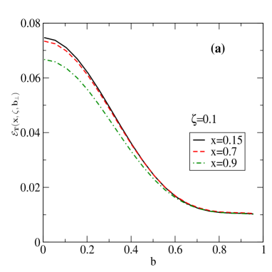
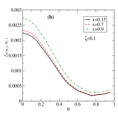
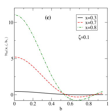
Figure 6: (Color online) Fourier spectrum of the chiral-odd GPDs vs. $\mid b_{\perp}\mid$ for fixed $\zeta$ and different values of $x$

The above picture was proposed in the limit of zero skewness $\zeta$ in burchi ; chiral . In most experiments $\zeta$ is nonzero, and it is of interest to investigate the chiral odd GPDs in $b_{\perp}$ space with nonzero $\zeta$. The probability interpretation is no longer possible as now the transverse position of the initial and final protons are different as there is a finite momentum transfer in the longitudinal direction. The GPDs in impact parameter space probe partons at transverse position $\mid b_{\perp}\mid$ with the initial and final proton shifted by an amount of order $\zeta\mid b_{\perp}\mid$. Note that this is independent of $x$ and and even when GPDs are integrated over $x$ in an amplitude, this information is still there markus2 . Thus the chiral odd GPDs in impact parameter space gives the spin orbit correlations of partons in protons with their centers shifted with respect to each other.

Taking the Fourier transform with respect to the transverse momentum transfer $\Delta_{\perp}$ we get the GPDs in the transverse impact parameter space.

$${\cal E}_{T}(x,\zeta,b_{\perp}) = {1\over(2\pi)^{2}}\int d^{2}\Delta_{\perp}e^{-i\Delta_{\perp}\cdot b_{\perp}}E_{T}(x,\zeta,t)$$ (36)

$$= {1\over 2\pi}\int\Delta d\Delta J_{0}(\Delta b)E_{T}(x,\zeta,t),$$

where $\Delta=|\Delta_{\perp}|$ and $b=|b_{\perp}|$. The other impact parameter dependent GPDs $\tilde{\cal E}_{T}(x,\zeta,b_{\perp})$ and ${\cal H}_{T}(x,\zeta,b_{\perp})$ can also be defined in the same way.

Fig.5 shows the chiral odd GPDs for nonzero $\zeta$ in impact parameter space for different $\zeta$ and fixed $x=0.5$ as a function of $\mid b_{\perp}\mid$. As $\zeta$ increases the peak at $\mid b_{\perp}\mid=0$ increases for $\tilde{\cal E}_{T}(x,\zeta,b_{\perp})$ but decreases for ${\cal H}_{T}(x,\zeta,b_{\perp})$ and ${\cal E}_{T}(x,\zeta,b_{\perp})$. It is to be noted that ${\cal H}_{T}(x,\zeta,b_{\perp})$ for a free Dirac particle is expected to be a delta function; the smearing in $\mid b_{\perp}\mid$ space is due to the spin correlation in the two-particle LFWFs. Fig. 6 shows the plots of the above three functions for fixed $\zeta$ and different values of $x$. For given $\zeta$, the peak of ${\cal H}_{T}(x,\zeta,b_{\perp})$ as well as $\tilde{\cal E}_{T}(x,\zeta,b_{\perp})$ increases with increase of $x$, however for ${\cal E}_{T}(x,\zeta,b_{\perp})$ it decreases.

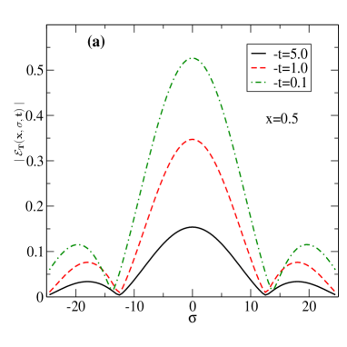
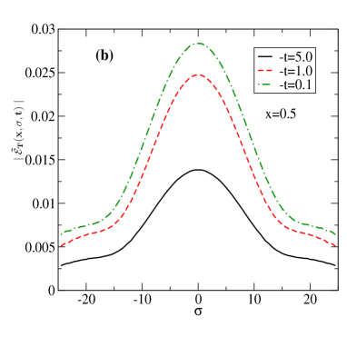
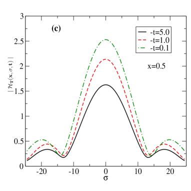
Figure 7: (Color online) Fourier spectrum of the chiral-odd GPDs vs. $\sigma$ for fixed $x$ and different values of $-t$ in ${\mathrm{MeV}^{2}}$.

So far, we discussed about the chiral odd GPDs in transverse position space. In wigner , a phase space distribution of quarks and gluons in the proton is given in terms of the quantum mechanical Wigner distribution $W(\vec{r},\vec{p})$, in the rest frame of the proton, which are functions of three position and three momentum coordinates. Wigner distributions are not accessible in experiment. However, if one integrates two momentum components one gets a reduced Wigner distribution $W_{\Gamma}(\vec{r},x)$ which is related to the GPDs by a Fourier transform. For given $x$, this gives a 3D position space picture of the partons inside the proton. In the infinite momentum frame, rotational symmetry is not there. Nevertheless, one can still define such a 3D position space distribution by taking a Fourier transform of the GPDs. Another point is the dynamical effect of Lorentz boosts. If the probing wavelength is comparable to or smaller than the Compton wavelength ${1\over M}$, where $M$ is the mass of the proton, electron-positron pairs will be created, as a result, the static size of the system cannot be probed to a precision better than ${1\over M}$ in relativistic quantum theory. However, in light-front theory, transverse boosts are Galilean boosts which do not involve dynamics. So one can still express the GPDs in transverse position or impact parameter space and this picture is not spoilt by relativistic corrections. However, rotation involves dynamics here and rotational symmetry is lost. In hadron_optics , a longitudinal boost invariant impact parameter $\sigma$ has been introduced which is conjugate to the longitudinal momentum transfer $\zeta$. It was shown that the DVCS amplitude expressed in terms of the variables $\sigma,b_{\perp}$ show diffraction pattern analogous to diffractive scattering of a wave in optics where the distribution in $\sigma$ measures the physical size of the scattering center in a 1-D system. In analogy with optics, it was concluded that the finite size of the $\zeta$ integration of the FT acts as a slit of finite width and produces the diffraction pattern.

We define a boost invariant impact parameter conjugate to the longitudinal momentum transfer as $\sigma={1\over 2}b^{-}P^{+}$ hadron_optics . The chiral odd GPD $E_{T}$ in longitudinal position space is given by :

$${\cal E}_{T}(x,\sigma,t) = {1\over 2\pi}\int_{0}^{\zeta_{f}}d\zeta e^{i{1\over 2}P^{+}\zeta b^{-}}E_{T}(x,\zeta,t)$$ (37)

$$= {1\over 2\pi}\int_{0}^{\zeta_{f}}d\zeta e^{i\sigma\zeta}E_{T}(x,\zeta,t).$$

Since we are concentrating only in the region $\zeta<x<1$, the upper limit of $\zeta$ integration $\zeta_{f}$ is given by $\zeta_{max}$ if $x$ is larger then $\zeta_{max}$, otherwise by $x$ if $x$ is smaller than $\zeta_{max}$ where $\zeta_{max}$ is the maximum value of $\zeta$ allowed for a fixed $-t$:

$$\zeta_{max}={(-t)\over 2M^{2}}\Big{(}\sqrt{1+{4M^{2}\over(-t)}}-1\Big{)}.$$ (38)

Similarly one can obtain ${\cal H}_{T}(x,\sigma,t)$ and $\tilde{\cal E}_{T}(x,\sigma,t)$ as well. Fig. 7 shows the plots of the Fourier spectrum of chiral odd GPDs in longitudinal position space as a function of $\sigma$ for fixed $x=0.5$ and different values of $t$. Both ${\cal E}_{T}(x,\sigma,t)$ and ${\cal H}_{T}(x,\sigma,t)$ show diffraction pattern as observed for the DVCS amplitude in hadron_optics ; the minima occur at the sames values of $\sigma$ in both cases. However $\tilde{\cal E}_{T}(x,\sigma,t)$ does not show diffraction pattern. This is due to the distinctively different behaviour of $\tilde{E}_{T}(x,\zeta,t)$ with $\zeta$ compared to that of $E_{T}(x,\zeta,t)$ and $H_{T}(x,\zeta,t)$. $\tilde{E}_{T}(x,\zeta,t)$ rises smoothly from zero and has no flat plateau in $\zeta$ and thus does not exhibit any diffraction pattern when Fourier transformed with respect to $\zeta$. The position of first minima in Fig.7 is determined by $\zeta_{f}$. For $-t=5.0$ and $1.0$, $\zeta_{f}\approx x=0.5$ and thus the first minimum appears at the same position while for $-t=0.1$, $\zeta_{f}=\zeta_{max}\approx 0.45$ and the minimum appears slightly shifted. This is analogous to the single slit optical diffraction pattern. $\zeta_{f}$ here plays the role of the slit width. Since the positions of the minima(measured from the centre of the diffraction pattern) are inversely proportional to the slit width, the minima move away from the centre as the slit width (i.e., $\zeta_{f}$) decreases. The optical analogy of the diffraction pattern in $\sigma$ space has been discussed in detail in hadron_optics in the context of DVCS amplitudes.

V Conclusion

In this work, we have studied the chiral-odd GPDs in transverse and longitudinal position space. Working in light-front gauge, we presented overlap formulas for the chiral odd GPDs in terms of proton light-front wave functions both in the DGLAP and ERBL regions. In the first case there is parton number conserving $n\to n$ overlap whereas in the latter case, parton number changes by two in $n+1\to n-1$ overlap. We investigated them in the DGLAP region, when the skewness $\zeta$ is less than $x$. We used a self consistent relativistic two-body model, namely the quantum fluctuation of an electron at one loop in QED. We used its most general form drell , where we have a different mass for the external electron and different masses for the internal electron and photon. The impact parameter space representations are obtained by taking Fourier transform of the GPDs with respect to the transverse momentum transfer. It is known that chiral ; burchi the chiral odd GPDs provide important information on the spin-orbit correlations of the transversely polarized partons in an unpolarized nucleon, as well as the correlations between the transverse quark spin and the nucleon spin in the transverse polarized nucleon. When $\zeta$ is non-zero, the initial and final proton are displaced in the impact parameter space relative to each other by an amount proportional to $\zeta$. As this is the region probed by most experiments, it is of interest to investigate this. By taking a Fourier transform with respect to $\zeta$ we presented the GPDs in the boost invariant longitudinal position space variable $\sigma$. $H_{T}$ and $E_{T}$ show diffraction pattern in $\sigma$ space. Further work is needed to investigate this behaviour and to study its model dependence.

VI acknowledgment

The work of DC is supported by Marie-Curie (IIF) Fellowship. AM thanks DST Fasttrack scheme, Govt. of India for financial support for completing this work.

References

(1) For reviews on generalized parton distributions,
and DVCS, see M. Diehl,
Phys. Rept, 388, 41 (2003); A. V. Belitsky and A. V. Radyushkin, Phys.
Rept. 418 1, (2005); K. Goeke, M.
V. Polyakov, M. Vanderhaeghen, Prog. Part. Nucl. Phys. 47, 401 (2001).
S. Boffi, B. Pasquini, Riv. Nuovo Cim. 30, 387, 2007.
(2) M. Burkardt, Int. J. Mod. Phys. A 18, 173 (2003);
M. Burkardt, Phys. Rev. D 62, 071503 (2000), Erratum-
ibid, D 66, 119903 (2002); J. P. Ralston and B. Pire, Phys. Rev. D 66, 111501 (2002).
(3) M. Burkardt, Phys. Rev. D 72, 094020 (2005).
(4) X. Ji. Phys. Rev. Lett. 78, 610 (1997).
(5) S. J. Brodsky, D. Chakrabarti, A. Harindranath,
A. Mukherjee and J. P. Vary, Phys. Lett. B 641, 440 (2006); Phys.
Rev. D 75, 014003 (2007).
(6) X. Ji, Phy. Rev. Lett. 91, 062001 (2003);
A. Belitsky, X. Ji, F. Yuan, Phys. Rev. D 69 074014
(2004).
(7) M. Diehl, Eur. Phys. J. C 19, 485 (2001).
(8) M. Diehl and P. Hagler, Eur.Phys.J.C 44, 87
(2005).
(9) D. Yu Ivanov, B. Pire, L. Szymanowski, O. V. Teryaev, Phys.
Lett. B 550, 65 (2002); R. Enberg, B. Pire, L. Szymanowski, Eur. Phy.
J C 47, 87 (2006).
(10) S. Ahmad, G. Goldstein, S. Liuti; arXiv:0805.3568.
(11) M. Gockeler et al. [QCDSF Collaboration and UKQCD Collaboration], Phys. Lett. B 627, 113 (2005); M. Gockeler et al.
[QCDSF and UKQCD collaboration], Phys. Rev. Lett. 98,
222001 (2007).
(12) S. Scopetta, Phys. Rev. D 72, 117502 (2005).
(13) B. Pasquini, M. Pincetti, S. Boffi, Phys. Rev. D 72,
094029 (2005).
(14) S. Meissner, A. Metz and K. Goeke,Phy. Rev. D 76,
034002 (2007).
(15) H. Dahiya, A. Mukherjee, Phys. Rev. D 77, 045032
(2008).
(16) S. J. Brodsky and S. D. Drell, Phys. Rev. D 22, 2236
(1980).
(17) A. Harindranath, R. Kundu, W. M. Zhang, Phys.
Rev. D 59, 094013 (1999); A. Harindranath, A. Mukherjee,
R. Ratabole, Phys. Lett. B 476, 471 (2000); Phys. Rev.
D 63, 045006 (2001).
(18) D. Chakrabarti and A. Mukherjee, Phys. Rev. D 71, 014038
(2005).
(19) D. Chakrabarti, A. Mukherjee, Phys. Rev. D 72,
034013 (2005).
(20) A. Mukherjee and M. Vanderhaeghen, Phys. Lett. B 542,
245 (2002), Phys. Rev. D 67, 085020 (2003).
(21) S. J. Brodsky, M. Diehl, D. S. Hwang, Nucl. Phys. B
596, 99 (2001); M. Diehl, T. Feldmann, R. Jacob, P. Kroll, Nucl. Phys.
B 596, 33 (2001), Erratum-ibid B 605, 647 (2001).
(22) S. J. Brodsky, D. S. Hwang, B-Q. Ma, I. Schmidt, Nucl. Phys.
B 593, 311 (2001).
(23) A. Mukherjee and D. Chakrabarti,
Phys. Lett. B 506, 283 (2001).
(24) H. Dahiya, A. Mukherjee, S. Ray, Phys. Rev. D 76, 034010
(2007).
(25) A. Mukherjee, I. V. Musatov, H. C. Pauli, A. V. Radyushkin,
Phys. Rev. D 67, 073014 (2003).