Relativistic corrections of $m\alpha^{6}(m/M)$ order to the hyperfine structure of the $\mbox{H}^{+}_{2}$ molecular ion

Abstract

The $m\alpha^{6}(m/M)$ order corrections to the hyperfine splitting in the $\mbox{H}_{2}^{+}$ ion are calculated. That allows to reduce uncertainty in the frequency intervals between hyperfine sublevels of a given rovibrational state to about 10 ppm. Results are in good agreement with the high precision experiment carried out by Jefferts in 1969.

I Introduction

In our previous work HFS06 we have calculated the hyperfine structure of the hydrogen molecular ion $\mbox{H}_{2}^{+}$ within the Breit-Pauli approximation taking account of the anomalous magnetic moment of an electron. This approximation includes the contributions of order $m\alpha^{4}(m/M)$ and $m\alpha^{5}(m/M)$ and thus the relative uncertainty in determination of the hyperfine structure intervals is of about $5\times 10^{-5}$. For the first time that has allowed to confirm the Jefferts measurements Jeff69 to the level of experimental accuracy of 1.5 kHz for transitions within the same multiplet $F$ ($F$ is the total spin of a state in ion). For the spin-flip transitions $(F=3/2)\to(F=1/2)$ a discrepancy of about 80 kHz still remains.

The main goal of the present work is to consider higher order corrections to the hyperfine splitting of $\mbox{H}_{2}^{+}$ to reduce the discrepancy with the Jefferts experiment for spin-flip lines down to a few ppm. To that end we will calculate the QED contributions of order $\alpha^{2}E_{F}$ and partially of order $\alpha^{3}E_{F}$ along with the proton finite size corrections such as Zemach and pure recoil contributions, which are essential at this level of accuracy.

The effective Hamiltonian of the spin interaction for the $\mbox{H}_{2}^{+}$ ion is (we use notation of HFS06 ):

$$\begin{array}[]{@{}l}\displaystyle H_{\rm eff}=b_{F}(\mathbf{I}\cdot\mathbf{s}_{e})+c_{e}(\mathbf{L}\cdot\mathbf{s}_{e})+c_{I}(\mathbf{L}\cdot\mathbf{I})+\frac{d_{1}}{(2L\!-\!1)(2L\!+\!3)}\biggl{\{}\frac{2}{3}\mathbf{L}^{2}(\mathbf{I}\cdot\mathbf{s}_{e})-[(\mathbf{L}\cdot\mathbf{I})(\mathbf{L}\cdot\mathbf{s}_{e})\!+\!(\mathbf{L}\cdot\mathbf{s}_{e})(\mathbf{L}\cdot\mathbf{I})]\biggr{\}}\\[8.53581pt] \displaystyle\hskip 170.71652pt+\frac{d_{2}}{(2L\!-\!1)(2L\!+\!3)}\left[\frac{1}{3}\mathbf{L}^{2}\mathbf{I}^{2}-\frac{1}{2}(\mathbf{L}\cdot\mathbf{I})-(\mathbf{L}\cdot\mathbf{I})^{2}\right],\end{array}$$ (1)

here $\mathbf{I}$ is the total nuclear spin, $\mathbf{L}$ is the total orbital momentum. The assumed coupling scheme of angular momenta is: $\mathbf{F}=\mathbf{I}+\mathbf{s}_{e}$, $\mathbf{J}=\mathbf{L}+\mathbf{F}$.

The major coupling is the spin-spin electron-proton interaction (first term in (1)) which determines the principal splitting between $F=1/2$ and $F=3/2$ states. So, the main contribution to the theoretical uncertainty on the spin-flip transition frequencies is uncertainty in the spin-spin interaction coefficient $b_{F}$, and our aim is to calculate an improved value for $b_{F}$.

Here it is very useful to make a comparison with the HFS studies of the hydrogen atom ground state. Indeed, the analytical form of many contributions to the hyperfine splitting of $\mbox{H}_{2}^{+}$ can be obtained from these results. Moreover, we will use the known results on the hydrogen atom as a guide and a check of our analytical derivations.

The hyperfine splitting for the ground state of a hydrogenlike atom may be obtained with high accuracy already from the nonrelativistic quantum mechanics (see for example BS ),

$$E_{F}=\frac{16}{3}\alpha^{2}cR_{\infty}\mu_{p}\frac{m_{e}}{M_{p}}\left[1+\frac{m_{e}}{M_{p}}\right]^{-3},$$ (2)

here $\mu_{p}$ is the magnetic moment of a proton in nuclear magnetons, $m_{e}$ and $M_{p}$ are the electron and proton masses, respectively. Quantum electrodynamics corrections without recoil terms have been known for some time SapYen ; Kin96 and may be expressed as:

$$\Delta E_{\mathrm{hfs,QED}}=E_{F}\left[1+a_{e}+\frac{3}{2}(Z\alpha)^{2}+\left(\ln{2}-\frac{5}{2}\right)\alpha(Z\alpha)-\frac{8}{3\pi}\alpha(Z\alpha)^{2}\ln^{2}(Z\alpha)+\dots\right],$$ (3)

where $a_{e}$ is the electron anomalous magnetic moment. We keep $Z$, the nuclear charge number, in all expressions in order to make clear the origins of different corrections.

Beyond pure QED corrections there are also proton structure effects (see SapYen ; Shabaev ; Carlson for a detailed discussion). The leading one is the Zemach correction Zemach ($(Z\alpha)(m/\Lambda)E_{F}$) that along with the radiative corrections to the nuclear structure contribution Karsh97 reads

$$\Delta E_{Z}=-2\frac{m_{e}M_{p}}{M_{p}+m_{e}}\left(Z\alpha\right)R_{Z}(1+\delta_{Z}^{\rm rad})E_{F},$$ (4)

Here $R_{Z}$ is the Zemach radius, a mean radius associated with the proton’s charge-current distribution,

$$R_{Z}=\frac{1}{\pi^{2}}\int\frac{d^{3}q}{q^{4}}\left[1-\frac{G_{E}(-q^{2})G_{M}(-q^{2})}{\mu_{p}}\right],$$

where $G_{E}$ and $G_{M}$ are the electric and magnetic form factors of a proton. We take $R_{Z}=1.045(16)$ fm Shabaev . Radiative corrections $\delta_{Z}^{\rm rad}$ to the Zemach contribution were obtained in Karsh97 and $\delta_{Z}^{\rm rad}=0.0153$. The parameter $\Lambda$ determines the energy scale that corresponds to the mean radius of the proton, and $\Lambda\approx 0.8M_{p}$ Karsh97 . Next are the pure recoil proton structure corrections of orders $(Z\alpha)^{k}(m/M)E_{F}$ ($k=1,2$) BodYen88

$$\Delta_{R}^{p}\approx(5.84\pm 0.01)\!\times\!10^{-6}\>E_{F}.$$ (5)

The last remaining effect of order $(Z\alpha)(m/M)E_{F}$, which has to be included, is the proton polarizability Fau02

$$\Delta_{\rm pol}\approx(1.4\pm 0.6)\!\times\!10^{-6}\>E_{F}.$$ (6)

A summary of various contributions to the HFS of the hydrogen ground state is given in Table 1. Up to now, in our previous studies for the $\mbox{H}_{2}^{+}$ ion HFS06 , only the contributions from the first two lines have been included into consideration. In the present work we intend to extend our research to higher order QED corrections (up to $E_{F}\,\alpha(Z\alpha)^{2}\ln^{2}(Z\alpha)$ term) as well as the proton structure effects.

term	(kHz)
$E_{F}$	$1418\,840.09$
$a_{e}E_{F}$	$1\,645.361$
$\Delta E_{(Z\alpha)^{2}}$	$113.333$
$\Delta E_{\alpha(Z\alpha)}$	$-136.517$
$\Delta E_{\alpha(Z\alpha)^{2}\ln^{2}(Z\alpha)}$	$-11.330$
higher order QED	$1.23$
$\Delta E_{Z}$	$-56.9(9)$
$\Delta E_{R}^{p}$	$8.43(8)$
$\Delta E_{\rm pol}$	$2.0(8)$
$\Delta E({\rm HFS})$	$1420\,405.7(1.7)$
experiment	$1420\,405.751\,7667(9)$

Table 1: Contributions to the hyperfine splitting of the ground state in a hydrogen atom. Uncertainty in the Fermi splitting, $E_{F}$, is determined by the fine structure constant. The second row is the contribution due to the anomalous magnetic moment of an electron, $a_{e}$. Contributions of higher orders, $(Z\alpha)^{2}$, $\alpha(Z\alpha)$, etc. as well as proton finite size corrections, are taken from Eqs. (3)-(6).

The major part of the contributions mentioned above in Eq. (4)-(6) may be considered as contact type interactions, which depend on the value of the squared density of the nonrelativistic wave function at the electron-proton coalescence point. Thus they do not require new extensive calculations, the mean values for the delta function operators can be taken from KorPRA06 . The main task is calculation of the relativistic correction term of order $E_{F}(Z\alpha)^{2}$, which may be performed using the nonrecoil limit of the two center problem. The obtained effective adiabatic potentials are subsequently averaged over the radial wave function as it was done for the $m\alpha^{6}$ order relativistic correction to ro-vibrational energies in KorJPB07 ; KorPRA08 .

The paper is organized as follows. In Sec. II.A and II.B we use the NRQED to derive all the spin-dependent interactions of order $\alpha^{6}(m/M)$ and the corresponding potentials in the coordinate space. The radiative corrections of orders $\alpha(Z\alpha)E_{F}$ and $\alpha(Z\alpha)^{2}\ln^{2}(Z\alpha)E_{F}$, as well as proton structure effects, which may be expressed as contact type interactions in the NRQED, are given in paragraph C. The perturbation formalism used to obtain the energy corrections is described in paragraph D. In the next two sections, we describe the calculation of the relativistic corrections of order $(Z\alpha)^{2}E_{F}$. First, for the HFS of the hydrogen ground state (Sec. III), where we rederive the well-known Breit correction Breit , providing a useful check of our approach. Then in Sec. IV the $\mbox{H}_{2}^{+}$ ion case is considered. Finally, numerical results are given and discussed in Sec. V.

II NRQED interactions

In this section we use the NRQED Cas86 to describe the interactions, which are of relevance to our problem. A nice and illuminative introduction to the NRQED approach may be found in Kin96 . The units $c=\hbar=1$ and $e^{2}=\alpha$ are used in this section, the elementary charge, $e$, is positive. We consider the low energy scattering, assuming that the momentum of a particle is of order $Z\alpha$, and we expand the scattering amplitude in terms of $\alpha$ and $\mathbf{p}^{2}$.

II.1 Tree-level interactions of order $m\alpha^{6}(m/M)$.

The momentum 4-vectors for the scattering of an electron (or proton) by the field of a static external source obey:

$$p_{0}^{\prime}=p_{0}=E,\qquad\mathbf{q}=\mathbf{p}^{\prime}-\mathbf{p},\qquad q_{0}=0,\qquad q^{2}=-\mathbf{q}^{2},$$

where $p$ and $p^{\prime}$ are 4-moments of incident and scattered particles, respectively.

On-shell Dirac spinors can be presented via the Schrödinger-Pauli spinors as follows

$$\begin{array}[]{@{}l}\displaystyle u(p)=\sqrt{\frac{E_{p}+m}{2E_{p}}}\left(\begin{matrix}\>X\\[2.84526pt] \frac{\boldsymbol{\sigma}^{P}\mathbf{p}}{E_{p}+m}\,X\end{matrix}\right),\qquad u^{*}(p)u(p)=(X^{*}X)=1,\\[8.53581pt] \displaystyle\hskip 99.58464ptE_{p}=\sqrt{m^{2}+\mathbf{p}^{2}}=m\left(1+\frac{\mathbf{p}^{2}}{2m^{2}}-\frac{\mathbf{p}^{4}}{8m^{4}}+\frac{\mathbf{p}^{6}}{16m^{6}}+\dots\right).\end{array}$$

here $\sigma^{P}_{i}$ are the two component Pauli matrices and $X$ are the two-component Schrödinger-Pauli wave functions. We assume that Dirac spinors are normalized as $(u^{*}u)=1$. That corresponds to the nonrelativistic normalization: the probability to discover a particle in a unit of volume is equal to unity. With this normalization Dirac spinors are expanded in the low-energy limit as follows

$$u(p)\approx\left(\begin{matrix}\left[1-\frac{\mathbf{p}^{2}}{8m^{2}}+\frac{11\mathbf{p}^{4}}{128m^{4}}\right]X\\[5.69054pt] \frac{\boldsymbol{\sigma}^{P}\mathbf{p}}{2m}\left[1-\frac{3\mathbf{p}^{2}}{8m^{2}}\right]X\end{matrix}\right).$$

The nonrelativistic scattering amplitude at tree-level for a scalar static field is determined by the following expansion

$$\begin{array}[]{@{}r@{\;}l}\displaystyle A_{E}(p,p^{\prime})&\displaystyle=X^{*}(\mathbf{p}^{\prime})(eZ)A_{0}(\mathbf{q})\biggl{(}1-\frac{\mathbf{q}^{2}}{8m^{2}}+i\frac{\boldsymbol{\sigma}^{P}[\mathbf{q}\times\mathbf{p}]}{4m^{2}}+\frac{3\mathbf{q}^{2}(p^{\prime 2}+p^{2})}{64m^{4}}\\[8.53581pt] &\displaystyle\hskip 76.82243pt+\frac{5(p^{\prime 2}-p^{2})^{2}}{128m^{4}}-i\frac{3\boldsymbol{\sigma}^{P}[\mathbf{q}\times\mathbf{p}](p^{\prime 2}+p^{2})}{32m^{4}}+\dots\biggr{)}X(\mathbf{p})\end{array}$$ (7)

and for a vector static field one obtains

$$\begin{array}[]{@{}r@{\;}l}\displaystyle A_{M}(p,p^{\prime})&\displaystyle=X^{*}(\mathbf{p}^{\prime})(eZ)\mathbf{A}(\mathbf{q})\biggl{(}-\frac{\mathbf{p}^{\prime}+\mathbf{p}}{2m}-i\frac{[\boldsymbol{\sigma}^{P}\times\mathbf{q}]}{2m}+\frac{\mathbf{p}^{\prime}(3p^{\prime 2}+p^{2})+\mathbf{p}(3p^{2}+p^{\prime 2})}{16m^{3}}\\[8.53581pt] &\displaystyle\hskip 76.82243pt+i\frac{[\boldsymbol{\sigma}^{P}\times\mathbf{p}^{\prime}](3p^{\prime 2}+p^{2})-[\boldsymbol{\sigma}^{P}\times\mathbf{p}](3p^{2}+p^{\prime 2})}{16m^{3}}+\dots\biggr{)}X(\mathbf{p})\end{array}$$ (8)

where $Z$ is the charge of a particle $e$, $p$,…For an electron $Z=-1$.

In what follows an index $a$ or $b=1,2$ denotes nucleus 1 or 2 in the $\mbox{H}_{2}^{+}$ ion, indices $i,j=1,3$ are Cartesian coordinates. The imaginary unit is denoted by upright $\mathrm{i}$.

The higher order vertices of tree level diagrams produce new interactions ($\mathbf{q}=\mathbf{p}^{\prime}_{e}\!-\!\mathbf{p}_{e}$):

a) via Coulomb photon exchange:

$$\mathcal{V}_{1}=e^{2}\left(\mathrm{i}\frac{3\boldsymbol{\sigma}_{e}^{P}[\mathbf{q}\times\mathbf{p}_{e}](p^{\prime 2}_{e}+p_{e}^{2})}{32m_{e}^{4}}\right)\frac{1}{\mathbf{q}^{2}}\;(Z_{a})$$ (9)

b) via transverse photon exchange:

$$\mathcal{V}_{2}=e^{2}\left(-\mathrm{i}\frac{[\boldsymbol{\sigma}^{P}_{e}\!\times\!\mathbf{p}^{\prime}_{e}](3p^{\prime 2}_{e}\!+\!p^{2}_{e})-[\boldsymbol{\sigma}^{P}_{e}\!\times\!\mathbf{p}_{e}](3p^{2}_{e}\!+\!p^{\prime 2}_{e})}{16m^{3}_{e}}\right)^{i}\left[-\frac{1}{\mathbf{q}^{2}}\left(\delta^{ij}-\frac{q^{i}q^{j}}{\mathbf{q}^{2}}\right)\right]\;\left(-Z_{a}\frac{\mathbf{P}_{a}^{\prime}+\mathbf{P}_{a}}{2M_{a}}\right)^{j}$$ (10a)

$$\mathcal{V}_{3}=e^{2}\left(-\frac{\mathbf{p}^{\prime}_{e}(3p^{\prime 2}_{e}+p^{2}_{e})+\mathbf{p}_{e}(3p^{2}_{e}+p^{\prime 2}_{e})}{16m^{3}_{e}}\right)^{i}\;\left[-\frac{1}{\mathbf{q}^{2}}\left(\delta^{ij}-\frac{q^{i}q^{j}}{\mathbf{q}^{2}}\right)\right]\;\left(-\mathrm{i}Z_{a}\frac{\boldsymbol{\sigma}_{a}^{P}\times(-\mathbf{q})}{2M_{a}}\right)^{j}$$ (10b)

$$\mathcal{V}_{4}=e^{2}\left(-\mathrm{i}\frac{[\boldsymbol{\sigma}^{P}_{e}\!\times\!\mathbf{p}^{\prime}_{e}](3p^{\prime 2}_{e}\!+\!p^{2}_{e})-[\boldsymbol{\sigma}^{P}_{e}\!\times\!\mathbf{p}_{e}](3p^{2}_{e}\!+\!p^{\prime 2}_{e})}{16m^{3}_{e}}\right)^{i}\left[-\frac{1}{\mathbf{q}^{2}}\left(\delta^{ij}-\frac{q^{i}q^{j}}{\mathbf{q}^{2}}\right)\right]\;\left(-\mathrm{i}Z_{a}\frac{\boldsymbol{\sigma}_{a}^{P}\times(-\mathbf{q})}{2M_{a}}\right)^{j}$$ (10c)

In parentheses here are the vertex functions of the effective NRQED interaction taken from Eqs. (7)-(8). The approximate transverse photon propagator (see BLP , § 83) is placed in the square brackets.

The obtained potentials can be simplified as follows:

$$\mathcal{V}_{2}=e^{2}\left(-\mathrm{i}\frac{2[\boldsymbol{\sigma}_{e}^{P}\!\times\!\mathbf{q}](p^{\prime 2}_{e}\!+\!p^{2}_{e})+[\boldsymbol{\sigma}_{e}^{P}\!\times\!(\mathbf{p}^{\prime}_{e}+\mathbf{p}_{e})](p^{\prime 2}_{e}\!-\!p^{2}_{e})}{16m_{e}^{3}}\right)^{i}\left[\frac{1}{\mathbf{q}^{2}}\left(\delta^{ij}-\frac{q^{i}q^{j}}{\mathbf{q}^{2}}\right)\right]\;\left(Z_{a}\frac{\mathbf{P}_{a}}{M_{a}}\right)^{j}$$

The last term in the first brackets produces a symmetric operator with the property: $(\varphi,A\varphi)=0$, for an arbitrary $\varphi$. That means that this operator is identical to zero operator, and $\mathcal{V}_{2}$ may be rewritten

$$\mathcal{V}_{2}=-e^{2}\left(\mathrm{i}\frac{[\boldsymbol{\sigma}_{e}^{P}\!\times\!\mathbf{q}](p^{\prime 2}_{e}\!+\!p^{2}_{e})}{8m_{e}^{3}}\right)^{i}\frac{1}{\mathbf{q}^{2}}\left(Z_{a}\frac{\mathbf{P}_{a}}{M_{a}}\right)^{i}$$ (11a)

In a similar way the other operators may be simplified:

$$\mathcal{V}_{3}=e^{2}\left(\frac{\mathbf{p}_{e}(p_{e}^{\prime 2}+p_{e}^{2})}{4m_{e}^{3}}\right)^{i}\frac{1}{\mathbf{q}^{2}}\left(\mathrm{i}\,Z_{a}\frac{\boldsymbol{\sigma}_{a}^{P}\!\times\!\mathbf{q}}{2M_{a}}\right)^{i}$$ (11b)

$$\mathcal{V}_{4}=-e^{2}\left(\frac{[\boldsymbol{\sigma}_{e}^{P}\!\times\!\mathbf{q}](p_{e}^{\prime 2}\!+\!p_{e}^{2})}{8m_{e}^{3}}\right)^{i}\frac{1}{\mathbf{q}^{2}}\left(Z_{a}\frac{\boldsymbol{\sigma}_{a}^{P}\!\times\!\mathbf{q}}{2M_{a}}\right)^{i}$$ (11c)

Transforming potentials $\mathcal{V}_{n}$ to the coordinate space ($\mathbf{r}_{a}=\mathbf{R}_{e}-\mathbf{R}_{a}$, where $\mathbf{R}_{e}$, $\mathbf{R}_{a}$ are the coordinates of electron and nuclei with respect to the center of mass) one gets, using the notation $\left\{A,B\right\}=AB+BA$:

$$\begin{array}[]{@{}l}\displaystyle\mathcal{V}_{1}=-\alpha\frac{3Z_{a}}{16m_{e}^{4}}\left\{p_{e}^{2},\frac{1}{r_{a}^{3}}[\mathbf{r}_{a}\!\times\!\mathbf{p}_{e}]\right\}\mathbf{s}_{e},\\[11.38109pt] \displaystyle\mathcal{V}_{2}=\alpha\frac{Z_{a}}{4m_{e}^{3}M_{a}}\left\{p_{e}^{2},\frac{1}{r_{a}^{3}}[\mathbf{r}_{a}\!\times\!\mathbf{P}_{a}]\right\}\mathbf{s}_{e},\\[11.38109pt] \displaystyle\mathcal{V}_{3}=-\alpha\frac{1}{2m_{e}^{3}}\left\{p_{e}^{2},\frac{1}{r_{a}^{3}}[\mathbf{r}_{a}\!\times\!\mathbf{p}_{e}]\right\}\boldsymbol{\mu}_{a},\\[11.38109pt] \displaystyle\mathcal{V}_{4}=-\alpha\frac{1}{4m_{e}^{3}}\left\{p_{e}^{2},\left[\frac{8\pi}{3}\mathbf{s}_{e}\boldsymbol{\mu}_{a}\delta(\mathbf{r}_{a})-\frac{r_{a}^{2}\mathbf{s}_{e}\boldsymbol{\mu}_{a}\!-\!3(\mathbf{s}_{e}\mathbf{r}_{a})(\boldsymbol{\mu}_{a}\mathbf{r}_{a})}{r_{a}^{5}}\right]\right\}.\end{array}$$ (12)

Here $\boldsymbol{\mu}_{a}$ is the magnetic moment operator for nucleus $a$. Only $\mathcal{V}_{4}$ involves both electron and nuclear spins and contributes to $b_{F}$.

        
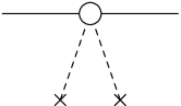
     $\displaystyle\frac{e^{2}\mathbf{E}^{2}}{8m^{3}}$ $\displaystyle\frac{e^{2}\boldsymbol{\sigma}\cdot[\mathbf{A}\times\mathbf{E}]}{4m^{2}}$ $\displaystyle\frac{e^{2}\mathbf{A}^{2}}{2m}$ $\alpha^{6}$ $\alpha^{6}\left(\frac{m}{M}\right)$ $\alpha^{6}\left(\frac{m}{M}\right)^{2}$

Figure 1: Top row: QED scattering diagrams. Bottom row: NRQED seagull interactions inferred from QED diagrams.

II.2 Seagull-type interactions

In Fig. 1, three NRQED seagull diagrams are presented. They may be obtained from the corresponding QED $Z$-diagrams by expanding the scattering amplitude in terms of $\mathbf{p}^{2}$. The double Coulomb photon exchange diagram has a leading order $\alpha^{6}$, however it does not involve interactions dependent on spin. The third diagram is double transverse photon exchange has a recoil order $(m/M)^{2}$, and is also out of interest for present consideration.

The potentials which stems from the seagull vertex with one Coulomb and one transverse photon lines can be expressed as follows ($\mathbf{q}_{1}=\mathbf{P}_{1}-\mathbf{P}^{\prime}_{1}$, $\mathbf{q}_{2}=\mathbf{P}_{2}-\mathbf{P}^{\prime}_{2}$):

$$\mathcal{V}_{5}=e^{4}\frac{\boldsymbol{\sigma}_{e}^{P}}{4m_{e}^{2}}\left[\left\{\left[-\frac{1}{\mathbf{q}_{b}^{2}}\left(\delta^{ij}-\frac{q_{b}^{i}q_{b}^{j}}{\mathbf{q}_{b}^{2}}\right)\right]\left(-Z_{b}\frac{\mathbf{P}^{\prime}_{b}+\mathbf{P}_{b}}{2M_{b}}\right)^{i}\right\}\times\mathrm{i}\left[\frac{\mathbf{q}_{a}}{\mathbf{q}_{a}^{2}}\right]^{j}(Z_{a})\right]$$ (13a)

$$\mathcal{V}_{6}=e^{4}\frac{\boldsymbol{\sigma}_{e}^{P}}{4m_{e}^{2}}\left[\left\{\left[-\frac{1}{\mathbf{q}_{b}^{2}}\left(\delta^{ij}-\frac{q_{b}^{i}q_{b}^{j}}{\mathbf{q}_{b}^{2}}\right)\right]\left(-\mathrm{i}Z_{b}\frac{\boldsymbol{\sigma}_{b}^{P}\times(-\mathbf{q}_{b})}{2M_{b}}\right)^{i}\right\}\times\mathrm{i}\left[\frac{\mathbf{q}_{a}}{\mathbf{q}_{a}^{2}}\right]^{j}(Z_{a})\right]$$ (13b)

The sources $Z_{a}$ and $Z_{b}$ may belong to a same particle or to two different particles.

In the coordinate space one has, for $a\neq b$,

$$\mathcal{V}_{5}=-\alpha^{2}\frac{Z_{a}Z_{b}}{4m_{e}^{2}M_{b}}\left\{\frac{[\mathbf{r}_{a}\!\times\!\mathbf{P}_{b}]}{r_{a}^{3}r_{b}}+\frac{[\mathbf{r}_{a}\!\times\!\mathbf{r}_{b}](\mathbf{r}_{b}\mathbf{P}_{b})}{r_{a}^{3}r_{b}^{3}}\right\}\mathbf{s}_{e}\,,$$ (14a)

$$\mathcal{V}_{6}=\alpha^{2}\frac{Z_{a}Z_{b}\mu_{b}}{2m_{e}^{2}M_{b}}\frac{[\mathbf{r}_{a}\!\times\!\mathbf{s}_{e}][\mathbf{r}_{b}\!\times\!\mathbf{s}_{b}]}{r_{a}^{3}r_{b}^{3}}=\alpha^{2}\frac{Z_{a}}{2m_{e}^{2}}\frac{[\mathbf{r}_{a}\!\times\!\mathbf{s}_{e}][\mathbf{r}_{b}\!\times\!\boldsymbol{\mu}_{b}]}{r_{a}^{3}r_{b}^{3}}\,.$$ (14b)

Using $$[\mathbf{a}\!\times\!\mathbf{b}][\mathbf{c}\!\times\!\mathbf{d}]=(\mathbf{ac})(\mathbf{bd})\!-\!(\mathbf{cb})(\mathbf{ad}) \mathcal{V}_{6}$$, one may further simplify .

When the sources coincide ($a=b$), the interactions modify as follows:

$$\mathcal{V}_{7}=-\alpha^{2}\frac{Z_{a}^{2}}{4m_{e}^{2}M_{a}}\frac{[\mathbf{r}_{a}\!\times\!\mathbf{P}_{a}]}{r_{a}^{4}}\mathbf{s}_{e}\,,$$ (14c)

$$\mathcal{V}_{8}=\alpha^{2}\frac{Z_{a}}{2m_{e}^{2}}\frac{[\mathbf{r}_{a}\!\times\!\mathbf{s}_{e}][\mathbf{r}_{a}\!\times\!\boldsymbol{\mu}_{a}]}{r_{a}^{6}}=-\alpha^{2}\frac{Z_{a}}{2m_{e}^{2}}\left[\frac{(\mathbf{r}_{a}\mathbf{s}_{e})(\mathbf{r}_{a}\boldsymbol{\mu}_{a})-(1/3)r_{a}^{2}(\mathbf{s}_{e}\boldsymbol{\mu}_{a})}{r_{a}^{6}}-\frac{2}{3}\frac{(\mathbf{s}_{e}\boldsymbol{\mu}_{a})}{r_{a}^{4}}\right].$$ (14d)

Among those terms, only $\mathcal{V}_{6}$ and $\mathcal{V}_{8}$ contribute to $b_{F}$.

II.3 Contact type NRQED interactions.

Here we introduce corrections already mentioned in the introduction, which enter into the NRQED Lagrangian as contact type interactions, since they reproduce effects of the relativistic scale.

• Radiative interactions of order $\alpha(Z\alpha)E_{F}$:

  $$V_{r}^{(6)}=\alpha^{3}\frac{8\pi Z}{3m_{e}}\frac{\mu_{p}}{M_{p}}\left(\ln{2}-\frac{13}{4}+\frac{3}{4}\right)\bigl{(}\mathbf{s}_{e}\cdot\mathbf{I}_{a}\bigr{)}\delta(\mathbf{r}_{a}),$$ (15)

  and of order $\alpha(Z\alpha)^{2}\ln^{2}(Z\alpha)E_{F}$

  $$V_{r}^{(7)}=\alpha^{4}\ln^{2}(Z\alpha)\frac{8\pi Z^{2}}{3m_{e}}\frac{\mu_{p}}{M_{p}}\left(-\frac{8}{3\pi}\right)\bigl{(}\mathbf{s}_{e}\cdot\mathbf{I}_{a}\bigr{)}\delta(\mathbf{r}_{a}).$$ (16)

• Zemach term ($(Z\alpha)(m/\Lambda)E_{F}$):

  $$V_{Z}=-2\alpha R_{Z}(1+\delta^{\rm rad}_{Z})\,\frac{8\pi Z}{3m_{e}}\frac{\mu_{p}}{M_{p}}\>\bigl{(}\mathbf{s}_{e}\cdot\mathbf{I}_{a}\bigr{)}\delta(\mathbf{r}_{a}).$$ (17)

  where $R_{Z}=1.045(16)$ Shabaev .

• Recoil correction of order $(Z\alpha)(m/M)E_{F}$ BodYen88 ; Shabaev :

  $$V_{recoil}=\alpha\left[5.48(6)\cdot 10^{-6}\right]\frac{8\pi}{3m_{e}}\frac{\mu_{p}}{M_{p}}\>\bigl{(}\mathbf{s}_{e}\cdot\mathbf{I}_{a}\bigr{)}\delta(\mathbf{r}_{a}).$$ (18)

  The correction of order $(Z\alpha)^{2}(m/M)E_{F}$ from Eq. (5) has been omitted since it has to be considered in the context of higher order corrections, which are out of the scope of present consideration.

• proton polarizability Fau02 :

  $$V_{pol}=\alpha\left[1.4(6)\cdot 10^{-6}\right]\frac{8\pi}{3m_{e}}\frac{\mu_{p}}{M_{p}}\>\bigl{(}\mathbf{s}_{e}\cdot\mathbf{I}_{a}\bigr{)}\delta(\mathbf{r}_{a}).$$ (19)

II.4 Perturbation formalism.

To calculate the bound state problem we use the nonrelativistic Rayleigh-Schrödinger perturbation theory, where the starting point, the zero order approximation, is the nonrelativistic Schrödinger equation:

$$H_{0}\Psi_{0}=E_{0}\Psi_{0},$$ (20)

and the perturbation is the effective Hamiltonian $H_{\rm eff}$ derived from the NRQED Lagrangian and

$$\Delta E=\left\langle H_{\rm eff}\right\rangle+\left\langle H_{\rm eff}Q(E_{0}-H_{0})^{-1}QH_{\rm eff}\right\rangle+\left\langle H_{\rm eff}\right\rangle\left\langle\left[\frac{\partial}{\partial E}H_{\rm eff}\right]\right\rangle+\dots$$ (21)

where $Q$ is a projector operator on the subspace orthogonal to the zero-order wave function. $H_{\rm eff}$ has contributions of different orders in $\alpha$:

$$H_{\rm eff}=H^{(4)}+H^{(5)}+H^{(6)}+\dots$$

Then for our case the complete contribution at order of $\alpha^{6}(m/M)$ to the hyperfine structure of hydrogen atom and ion can be expressed by

$$\Delta E_{\rm hfs}=\left\langle H^{(6)}\right\rangle+\left\langle H_{u}^{(4)}Q(E_{0}-H_{0})^{-1}QH_{v}^{(4)}\right\rangle.$$ (22)

where $H_{u}^{(4)}$ and $H_{v}^{(4)}$ are parts of the Breit-Pauli Hamiltonian taken so that the second term in (22) contributes to that particular order. Since the effective Hamiltonian $H^{(6)}$ for the HFS does not depend on $E$ explicitly, the last term of Eq. (21) vanishes. In the following, the second-order contribution and the first-order contribution $\langle H^{(6)}\rangle$ will be denoted $\Delta E_{A}$ and $\Delta E_{B}$, respectively.

III HFS in the hydrogen ground state

In the remaining part of this work we will be using the atomic units ($e=\hbar=1$ and $c=\alpha^{-1}$). First, we consider the case of the HFS of the ground state of a hydrogen atom. Our derivation is somewhat similar to the one done by Nio and Kinoshita in Kin97 . The divergent part is, however, treated in a different way by explicitly separating out and cancelling the divergences. We start from the nonrelativistic Schrödinger equation:

$$(H_{0}-E_{0})\Psi_{0}=\left(\frac{p_{e}^{2}}{2m_{e}}+V\right)\Psi_{0},$$ (23)

where

$$V=-\frac{Z}{r}.$$ (24)

III.1 Separating divergences in the $m\alpha^{6}(m/M)$ order effective Hamiltonian

The effective Hamiltonian of order $m\alpha^{6}(m/M)$ is obtained from Eqs. (12) and (14), interactions $\mathcal{V}_{4}$ and $\mathcal{V}_{8}$, expressed in atomic units. It has the form:

$$\begin{array}[]{@{}r@{\;}l}H^{(6)}&\displaystyle=\alpha^{4}\frac{2}{3m_{e}}\left[-\frac{1}{4m_{e}^{2}}\Bigl{\{}p_{e}^{2},4\pi\delta(\mathbf{r})\Bigr{\}}+\frac{Z}{2m_{e}}\;\frac{1}{r^{4}}\right]\mathbf{s}_{e}\boldsymbol{\mu}_{p}\end{array}$$ (25)

where $\boldsymbol{\mu}_{p}=(\mu_{p}/M_{p})\,\mathbf{I}_{p}$, then using the relation

$$\left\langle Z^{2}/r^{4}\right\rangle=-\left\langle\left(\mathbf{p}_{e}V\right)^{2}\right\rangle=-\left\langle\frac{p_{e}^{2}V^{2}+V^{2}p_{e}^{2}}{2}\right\rangle+\left\langle\mathbf{p}_{e}V^{2}\mathbf{p}_{e}\right\rangle-4\pi Z\left\langle V\delta(\mathbf{r})\right\rangle$$ (26)

obtained by integration by parts, and equation $p_{e}^{2}\Psi_{0}=2(E_{0}-V)\Psi_{0}$, one gets:

$$\Delta E^{(6)}_{B}=\left\langle H^{(6)}\right\rangle=\alpha^{4}\frac{2}{3Zm_{e}}\frac{\mu_{p}}{M_{p}}\biggl{[}\frac{2\pi Z\left\langle V\delta(\mathbf{r})\right\rangle}{m_{e}}+\bigl{\langle}V^{3}\bigr{\rangle}-E_{0}\bigl{\langle}V^{2}\bigr{\rangle}+\frac{\bigl{\langle}\mathbf{p}_{e}V^{2}\mathbf{p}_{e}\bigr{\rangle}}{2m_{e}}-\frac{4\pi ZE_{0}\left\langle\delta(\mathbf{r})\right\rangle}{m_{e}}\biggr{]}\left\langle\mathbf{s}_{e}\!\cdot\!\mathbf{I}_{p}\right\rangle.$$ (27)

In Eq. (27), the divergent contributions are now explicitly collected in the first two terms.

III.2 Separating divergences in the second order contribution

The second order contribution of order $m\alpha^{6}(m/M)$ to the spin-spin interaction can be easily identified from various combinations of terms of the Breit-Pauli Hamiltonian and may be written:

$$\Delta E_{A}^{(6)}=2\alpha^{4}\left\langle-\frac{\mathbf{p}_{e}^{4}}{8m_{e}^{3}}+\frac{Z}{8m_{e}^{2}}\,4\pi\delta(\mathbf{r})\bigg{|}Q(E_{0}-H_{0})^{-1}Q\bigg{|}\frac{8\pi}{3m_{e}}\;\mathbf{s}_{e}\boldsymbol{\mu}_{p}\,\delta(\mathbf{r})\right\rangle,$$ (28)

This contribution is divergent due to presence of the delta-function operators on both sides of the second order iteration.

Let us consider the two operators:

$$H_{B}^{(1)}=4\pi\delta(\mathbf{r}),\qquad H_{B}^{(2)}=-\frac{\mathbf{p}_{e}^{4}}{8m_{e}^{3}}+\frac{Z}{8m_{e}^{2}}\,4\pi\delta(\mathbf{r}),$$

and introduce the wavefunction $\Psi_{B}^{(1)}$ solution of equation

$$(E_{0}-H_{0})\Psi_{B}^{(1)}=Q\left[4\pi\,\delta(\mathbf{r})\right]\Psi_{0}=QH_{B}^{(1)}\Psi_{0}.$$ (29)

$\Psi_{B}^{(1)}$ behaves as $1/r$ at $r\to 0$. We introduce a less singular function $\tilde{\Psi}_{B}^{(1)}$ defined by

$$\Psi_{B}^{(1)}=-\frac{2m_{e}\Psi_{0}}{r}+\tilde{\Psi}_{B}^{(1)}=U_{1}\Psi_{0}+\tilde{\Psi}_{B}^{(1)},$$ (30)

where $U_{1}=-\frac{2m_{e}}{r}=\frac{2m_{e}}{Z}V$. The function $\tilde{\Psi}_{B}^{(1)}$ behaves as $\ln{r}$ at $r\to 0$. It satisfies equation

$$(E_{0}-H_{0})\tilde{\Psi}_{B}^{(1)}=\left({H^{\prime}_{B\!}}^{(1)}-\left\langle{H^{\prime}_{B\!}}^{(1)}\right\rangle\right)\Psi_{0},$$ (31)

where

$${H^{\prime}_{B\!}}^{(1)}=-(E_{0}-H_{0})U_{1}-U_{1}(E_{0}-H_{0})+H_{B}^{(1)}.$$ (32)

Similar computations can be applied to the scalar part of the Breit-Pauli Hamiltonian $H_{B}^{(2)}$:

$$\begin{array}[]{@{}l}\displaystyle(E_{0}-H_{0})\Psi_{B}^{(2)}=Q\left[-\frac{p^{4}}{8m_{e}^{3}}+\frac{Z\pi}{2m_{e}^{2}}\delta(\mathbf{r})\right]\Psi_{0}\\[11.38109pt] \displaystyle\Psi_{B}^{(2)}=\frac{Z\Psi_{0}(r)}{4m_{e}r}+\tilde{\Psi}_{B}^{(2)}=U_{2}\Psi_{0}+\tilde{\Psi}_{B}^{(2)},\qquad U_{2}=\frac{Z}{4m_{e}r}=-\frac{1}{4m_{e}}V.\end{array}$$ (33)

and

$${H^{\prime(2)}_{B\!}}=-(E_{0}-H_{0})U_{2}-U_{2}(E_{0}-H_{0})+H_{B}^{(2)}.$$ (34)

Using systematically that

$$\left\langle\Psi_{0}\Big{|}H_{B}^{(2)}Q(E_{0}-H_{0})^{-1}QH_{B}^{(1)}\Big{|}\Psi_{0}\right\rangle=\left\langle\Psi_{0}\Big{|}H_{B}^{(2)}Q\Big{|}\Psi_{B}^{(1)}\right\rangle,\qquad\mbox{or}\quad\left\langle\Psi_{B}^{(2)}\Big{|}QH_{B}^{(1)}\Big{|}\Psi_{0}\right\rangle,$$

one may separate the divergent singularities in the following way:

$$\begin{array}[]{@{}r@{\;}l}\Delta E_{A}&=\displaystyle\alpha^{4}\frac{4\mu_{p}}{3m_{e}M_{p}}\;\left\langle\mathbf{s}_{e}\!\cdot\!\mathbf{I}_{p}\right\rangle\left\langle\Psi_{0}\Big{|}H_{B}^{(2)}Q(E_{0}-H_{0})^{-1}QH_{B}^{(1)}\Big{|}\Psi_{0}\right\rangle\\[8.53581pt] &\displaystyle=\alpha^{4}\frac{2\mu_{p}}{3m_{e}M_{p}}\;\left\langle\mathbf{s}_{e}\!\cdot\!\mathbf{I}_{p}\right\rangle\left(2\left\langle\Psi_{0}\Big{|}\left(H_{B}^{(2)}-\left\langle H_{B}^{(2)}\right\rangle\right)U_{1}\Big{|}\Psi_{0}\right\rangle+2\left\langle\Psi_{0}\Big{|}\left(H_{B}^{(2)}-\left\langle H_{B}^{(2)}\right\rangle\right)\Big{|}\tilde{\Psi}_{B}^{(1)}\right\rangle\right)\\[8.53581pt] &\displaystyle=\alpha^{4}\frac{2\mu_{p}}{3m_{e}M_{p}}\;\left\langle\mathbf{s}_{e}\!\cdot\!\mathbf{I}_{p}\right\rangle\Bigl{(}2\left\langle\Psi_{0}\Big{|}\left(H_{B}^{(2)}-\left\langle H_{B}^{(2)}\right\rangle\right)U_{1}\Big{|}\Psi_{0}\right\rangle+2\left\langle\Psi_{0}\Big{|}H_{B}^{(2)}Q(E_{0}-H_{0})^{-1}Q{H^{\prime}_{B\!}}^{(1)}\Big{|}\Psi_{0}\right\rangle\Bigr{)}\\[8.53581pt] &\displaystyle=\alpha^{4}\frac{2\mu_{p}}{3m_{e}M_{p}}\;\ \left\langle\mathbf{s}_{e}\!\cdot\!\mathbf{I}_{p}\right\rangle\Bigl{(}2\left\langle\Psi_{0}\Big{|}\left(H_{B}^{(2)}-\left\langle H_{B}^{(2)}\right\rangle\right)U_{1}\Big{|}\Psi_{0}\right\rangle+2\left\langle\Psi_{0}\Big{|}U_{2}({H^{\prime}_{B\!}}^{(1)}-\langle{H^{\prime}_{B\!}}^{(1)}\rangle)\Big{|}\Psi_{0}\right\rangle\\[8.53581pt] &\displaystyle\hskip 128.0374pt+2\left\langle\Psi_{0}\Big{|}{H^{\prime}_{B\!}}^{(2)}Q(E_{0}-H_{0})^{-1}Q{H^{\prime}_{B\!}}^{(1)}\Big{|}\Psi_{0}\right\rangle\Bigr{)}\end{array}$$ (35)

The first two terms of the last expression may be rewritten as the average of a new effective Hamiltonian contributing to the $m\alpha^{6}(m/M)$ order:

$$\begin{array}[]{@{}r@{\;}l}\displaystyle H^{\prime(6)}&\displaystyle=\alpha^{4}\frac{2\mu_{p}}{3m_{e}M_{p}}\biggl{\{}\left(H_{B}^{(2)}U_{1}+U_{1}H_{B}^{(2)}\right)+\left(H_{B}^{(1)}U_{2}+U_{2}H_{B}^{(1)}\right)-2\left\langle H_{B}^{(2)}\right\rangle U_{1}-2\left\langle H_{B}^{(1)}\right\rangle U_{2}\\[5.69054pt] &\hskip 184.9429pt-U_{1}(E_{0}-H_{0})U_{2}-U_{2}(E_{0}-H_{0})U_{1}\biggr{\}}\left\langle\mathbf{s}_{e}\!\cdot\!\mathbf{I}_{p}\right\rangle.\end{array}$$ (36)

Using regularization and integration by parts in a similar way as in Appendix B of KorJPB07 its expectation value may be finally written in the form

$$\begin{array}[]{@{}r@{\;}l}\displaystyle\left\langle H^{\prime(6)}\right\rangle&\displaystyle=\alpha^{4}\frac{2\mu_{p}}{3Zm_{e}M_{p}}\biggl{[}-\frac{2\pi Z\left\langle V\delta(\mathbf{r})\right\rangle}{m_{e}}-\left\langle V^{3}\right\rangle+\frac{\left\langle\mathbf{p}V^{2}\mathbf{p}\right\rangle}{2m_{e}}+3E_{0}\left\langle V^{2}\right\rangle-2E_{0}^{2}\left\langle V\right\rangle\\[2.84526pt] &\hskip 213.39566pt\displaystyle-4m_{e}\left\langle H_{B}^{(2)}\right\rangle\langle V\rangle+\frac{Z\bigl{\langle}H_{B}^{(1)}\bigr{\rangle}\langle V\rangle}{2m_{e}}\biggr{]}\left\langle\mathbf{s}_{e}\!\cdot\!\mathbf{I}_{p}\right\rangle.\end{array}$$ (37)

All the divergent terms of Eq. (35) are collected as the first two terms of Eq. (37). They clearly cancel out those of Eq. 27.

The remaining part of the second order iteration contribution (the last term in Eq. (35)) is finite

$$\Delta E^{\prime(6)}_{A}=\alpha^{4}\frac{4\mu_{p}}{3m_{e}M_{p}}\left\langle\Psi_{0}\Big{|}{H^{\prime}_{B\!}}^{(2)}Q(E_{0}-H_{0})^{-1}Q{H^{\prime}_{B\!}}^{(1)}\Big{|}\Psi_{0}\right\rangle\left\langle\mathbf{s}_{e}\!\cdot\!\mathbf{I}_{p}\right\rangle,$$ (38)

where ${H^{\prime}_{B\!}}^{(1)}$ and ${H^{\prime}_{B\!}}^{(2)}$ are defined above in Eqs. (32) and (34), respectively.

Summing up $\left\langle H^{(6)}\right\rangle$ and $\left\langle H^{\prime(6)}\right\rangle$ from Eqs. (27) and (37) one gets a finite expression as well

$$\begin{array}[]{@{}l}\displaystyle\Delta E^{\prime(6)}_{B}=\alpha^{4}\frac{2\mu_{p}}{3Zm_{e}M_{p}}\biggl{[}\frac{\left\langle\mathbf{p}V^{2}\mathbf{p}\right\rangle}{m_{e}}+2E_{0}\left\langle V^{2}\right\rangle-2E_{0}^{2}\left\langle V\right\rangle-\frac{ZE_{0}}{m_{e}}\>4\pi\left\langle\delta(\mathbf{r})\right\rangle\\[8.53581pt] \hskip 199.16928pt\displaystyle-4m_{e}\left\langle H_{B}^{(2)}\right\rangle\langle V\rangle+\frac{Z\bigl{\langle}H_{B}^{(1)}\bigr{\rangle}\langle V\rangle}{2m_{e}}\biggr{]}\left\langle\mathbf{s}_{e}\!\cdot\!\mathbf{I}_{p}\right\rangle.\end{array}$$ (39)

III.3 Calculation of expectation values and final result

We now check that Eq. (39) leads to the usual result in the case of an 1s hydrogen atom. Here, $\Psi_{0}=2Z^{3/2}e^{-Zr}$ is the ground state wave function. First we look for a solution of equation:

$$(E_{0}-H_{0})\tilde{\Psi}_{B}^{(1)}=\left(\!{H^{\prime}_{B\!}}^{(1)}\!-\!\left\langle{\!H^{\prime}_{B\!}}^{(1)}\!\right\rangle\right)\Psi_{0},\qquad{H^{\prime}_{B\!}}^{(1)}=-\frac{2}{r^{2}}\partial_{r}\!-2U_{1}(E_{0}\!-\!H_{0}),\qquad\left\langle\!H_{B}^{(1)}\!\right\rangle=4Z^{3},$$

and get

$$\tilde{\Psi}_{B}^{(1)}=4Z(\ln{r}-1+Zr)\Psi_{0}.$$

The next step is to calculate the expectation value of

$$\left\langle\Psi_{0}\left|{H^{\prime}_{B\!}}^{(2)}Q\right|\tilde{\Psi}_{B}^{(1)}\right\rangle=\left\langle\Psi_{0}\left|{H^{\prime}_{B\!}}^{(2)}\!-\left\langle{\!H^{\prime}_{B\!}}^{(2)}\!\right\rangle\right|\tilde{\Psi}_{B}^{(1)}\right\rangle,$$

and to get the finite part of the second order contribution

$$\Delta E^{\prime(6)}_{A}=\frac{4Zm_{e}\alpha^{4}}{3}\frac{\mu_{p}}{M_{p}}\left\langle\Psi_{0}\Big{|}{H^{\prime}_{B\!}}^{(2)}Q(E_{0}-H_{0})^{-1}Q{H^{\prime}_{B\!}}^{(1)}\Big{|}\Psi_{0}\right\rangle\left\langle\mathbf{s}_{e}\!\cdot\!\mathbf{I}_{p}\right\rangle=\frac{3(Z\alpha)^{2}}{2}E_{F}\left\langle\mathbf{s}_{e}\!\cdot\!\mathbf{I}_{p}\right\rangle.$$

The expectation values of the operators involved in $\Delta E^{\prime(6)}_{B}$ are $\langle\mathbf{p}V^{2}\mathbf{p}\rangle=Z^{2}\langle V^{2}\rangle$, $\langle V^{2}\rangle=2Z^{2}$, and $\langle V\rangle=-Z$. This contribution is immediately obtained to be 0, indeed

$$\Delta E^{\prime(6)}_{B}=\frac{2Zm_{e}\alpha^{4}}{3}\frac{\mu_{p}}{M_{p}}\left[2Z^{5}\!-\!2Z^{5}\!+\!\frac{Z^{5}}{2}\!+\!2Z^{5}\!-\!\frac{Z^{5}}{2}\!-\!2Z^{5}\right]\left\langle\mathbf{s}_{e}\!\cdot\!\mathbf{I}_{p}\right\rangle=0.$$

Thus, the total contribution is

$$\Delta E^{(6)}=\Delta E^{\prime(6)}_{A}+\Delta E^{\prime(6)}_{B}=\frac{3}{2}(Z\alpha)^{2}E_{F}\left\langle\mathbf{s}_{e}\!\cdot\!\mathbf{I}_{p}\right\rangle.$$

that exactly matches the well-known Breit relativistic correction Breit .

IV Hydrogen molecular ion $\mbox{H}_{2}^{+}$

Now we are ready to study the hydrogen molecular ion. As in the previous section we start from the nonrelativistic equation with the Hamiltonian:

$$H_{0}=\frac{p^{2}}{2m_{e}}+V,\qquad V=-\frac{Z_{1}}{r_{1}}-\frac{Z_{2}}{r_{2}}.$$ (40)

We will assume here that $Z_{1}\!=\!Z_{2}\!=\!Z$ and $\boldsymbol{\mu}_{1}\!=\!(\mu_{p}/M_{p})\mathbf{I}_{1}$, $\boldsymbol{\mu}_{2}\!=\!(\mu_{p}/M_{p})\mathbf{I}_{2}$, where $\mathbf{I}_{1}$ and $\mathbf{I}_{2}$ are the two proton spin operators.

The second order contribution of the spin-spin interaction of order $m\alpha^{6}(m/M)$ is expressed by

$$\Delta E_{A}=2\alpha^{4}\left\langle-\frac{\mathbf{p}_{e}^{4}}{8m_{e}^{3}}+\frac{Z}{8m_{e}^{2}}\,4\pi\left[\delta(\mathbf{r}_{1})\!+\!\delta(\mathbf{r}_{2})\right]\bigg{|}Q(E_{0}-H_{0})^{-1}Q\bigg{|}\frac{8\pi}{3m_{e}}\;\mathbf{s}_{e}\left[\boldsymbol{\mu}_{1}\delta(\mathbf{r}_{1})\!+\!\boldsymbol{\mu}_{2}\delta(\mathbf{r}_{2})\right]\right\rangle$$ (41)

The effective Hamiltonian of order $m\alpha^{6}(m/M)$ is obtained from Eqs. (12) and (14) of Sec. II. Now we have three interactions, $\mathcal{V}_{4}$, $\mathcal{V}_{6}$, and $\mathcal{V}_{8}$, because we have as well the seagull interaction $\mathcal{V}_{6}$ with two different nuclei,

$$\mathcal{V}_{4a}=-\alpha^{4}\frac{1}{4m_{e}^{3}}\left\{p_{e}^{2},\left[\frac{8\pi}{3}\mathbf{s}_{e}\boldsymbol{\mu}_{a}\delta(\mathbf{r}_{a})-\frac{r_{a}^{2}\mathbf{s}_{e}\boldsymbol{\mu}_{a}\!-\!3(\mathbf{s}_{e}\mathbf{r}_{a})(\boldsymbol{\mu}_{a}\mathbf{r}_{a})}{r_{a}^{5}}\right]\right\},$$ (42a)

$$\mathcal{V}_{6}=\alpha^{4}\frac{Z}{6m_{e}^{2}}\left\{\frac{2(\mathbf{r}_{1}\mathbf{r}_{2})(\mathbf{s}_{e}\boldsymbol{\mu}_{I})}{r_{1}^{3}r_{2}^{3}}+\frac{(\mathbf{r}_{1}\mathbf{r}_{2})(\mathbf{s}_{e}\boldsymbol{\mu}_{I})\!-\!3(\mathbf{r}_{1}\mathbf{s}_{e})(\mathbf{r}_{2}\boldsymbol{\mu}_{2})\!-\!3(\mathbf{r}_{2}\mathbf{s}_{e})(\mathbf{r}_{1}\boldsymbol{\mu}_{1})}{r_{1}^{3}r_{2}^{3}}\right\},$$ (42b)

$$\mathcal{V}_{8a}=\alpha^{4}\frac{Z}{6m_{e}^{2}}\;\left[\frac{2(\mathbf{s}_{e}\boldsymbol{\mu}_{a})}{r_{a}^{4}}+\frac{r_{a}^{2}(\mathbf{s}_{e}\boldsymbol{\mu}_{a})\!-\!3(\mathbf{r}_{a}\mathbf{s}_{e})(\mathbf{r}_{a}\boldsymbol{\mu}_{a})}{r_{a}^{6}}\right],$$ (42c)

where $\boldsymbol{\mu}_{I}=\boldsymbol{\mu}_{1}+\boldsymbol{\mu}_{2}$. It is convenient to separate the effective Hamiltonian into two terms: scalar and tensor,

$$\begin{array}[]{@{}r@{\;}l}H_{s}^{(6)}&\displaystyle=\alpha^{4}\frac{Z}{3m_{e}}\frac{\mu_{p}}{m_{p}}\left[-\frac{1}{4m_{e}^{2}}\Bigl{\{}p_{e}^{2},4\pi\left[\delta(\mathbf{r}_{1})\!+\!\delta(\mathbf{r}_{1})\right]\Bigr{\}}+\frac{Z}{2m_{e}}\left(\frac{1}{r_{1}^{4}}+\frac{1}{r_{2}^{4}}+\frac{2\mathbf{r}_{1}\mathbf{r}_{2}}{r_{1}^{3}r_{2}^{3}}\right)\right]\left(\mathbf{s}_{e}\!\cdot\mathbf{I}\right)\\[8.53581pt] H_{t}^{(6)}&\displaystyle=\alpha^{4}\frac{Z}{6m_{e}}\Biggl{[}\frac{r_{1}^{2}(\mathbf{s}_{e}\boldsymbol{\mu}_{2})\!-\!3(\mathbf{r}_{1}\mathbf{s}_{e})(\mathbf{r}_{1}\boldsymbol{\mu}_{1})}{r_{1}^{6}}+\frac{r_{2}^{2}(\mathbf{s}_{e}\boldsymbol{\mu}_{2})\!-\!3(\mathbf{r}_{2}\mathbf{s}_{e})(\mathbf{r}_{2}\boldsymbol{\mu}_{2})}{r_{2}^{6}}\\[8.53581pt] &\displaystyle\hskip 56.9055pt+\frac{(\mathbf{r}_{1}\mathbf{r}_{2})(\mathbf{s}_{e}\boldsymbol{\mu}_{I})\!-\!3(\mathbf{r}_{1}\mathbf{s}_{e})(\mathbf{r}_{2}\boldsymbol{\mu}_{2})\!-\!3(\mathbf{r}_{2}\mathbf{s}_{e})(\mathbf{r}_{1}\boldsymbol{\mu}_{2})}{r_{1}^{3}r_{2}^{3}}\Biggr{]}.\end{array}$$ (43)

$H_{t}^{(6)}$ has a finite expectation value, and since it does not contribute to $b_{F}$, its consideration will be omitted in what follows. The divergent terms are encountered only in the scalar Hamiltonian.

IV.1 Separating divergences in the second order contribution

The operators which appear on the left and on the right of the second order iteration are:

$$H_{B}^{(1)}=4\pi\Bigl{(}\delta(\mathbf{r}_{1})+\delta(\mathbf{r}_{2})\Bigr{)},\qquad H_{B}^{(2)}=-\frac{\mathbf{p}_{e}^{4}}{8m_{e}^{3}}+\frac{Z}{8m_{e}^{2}}\,4\pi\Bigl{(}\delta(\mathbf{r}_{1})+\delta(\mathbf{r}_{2})\Bigr{)}.$$

Now we have to separate the singular part using the method outlined in the hydrogen case. We set :

$$\begin{array}[]{@{}l}\displaystyle(E_{0}-H_{0})\Psi_{B}^{(1)}=Q\left[4\pi\,\Bigl{(}\delta(\mathbf{r}_{1})+\delta(\mathbf{r}_{2})\Bigr{)}\right]\Psi_{0}\\[8.53581pt] \displaystyle\Psi_{B}^{(1)}=2m_{e}\left[-\frac{1}{r_{1}}-\frac{1}{r_{2}}\right]\Psi_{0}+\tilde{\Psi}_{B}^{(1)}=U_{1}\Psi_{0}+\tilde{\Psi}_{B}^{(1)},\qquad U_{1}=\frac{2m_{e}}{Z}V,\\[11.38109pt] \displaystyle H^{\prime(1)}_{B}=-(E_{0}-H_{0})U_{1}-U_{1}(E_{0}-H_{0})+H_{B}^{(1)}.\end{array}$$ (44)

Similarly, one gets for $H^{(2)}_{B}$:

$$\begin{array}[]{@{}l}\displaystyle(E_{0}-H_{0})\Psi_{B}^{(2)}=Q\left[-\frac{p^{4}}{8m_{e}^{3}}+\frac{Z\pi}{2m_{e}^{2}}\Bigl{(}\delta(\mathbf{r}_{1})+\delta(\mathbf{r}_{2})\Bigr{)}\right]\Psi_{0}\\[8.53581pt] \displaystyle\Psi_{B}^{(2)}=\frac{Z}{4m_{e}}\left[-\frac{1}{r_{1}}-\frac{1}{r_{2}}\right]\Psi_{0}(r)+\tilde{\Psi}_{B}^{(2)}=U_{2}\Psi_{0}+\tilde{\Psi}_{B}^{(2)},\qquad U_{2}=-\frac{1}{4m_{e}}V.\\[11.38109pt] \displaystyle H^{\prime(2)}_{B}=-(E_{0}-H_{0})U_{2}-U_{2}(E_{0}-H_{0})+H_{B}^{(2)}\end{array}$$ (45)

Applying these transformations to the second order iteration term we arrive at

$$\begin{array}[]{@{}r@{\;}l}\Delta E_{A}&=\displaystyle\alpha^{4}\frac{2}{3m_{e}}\frac{\mu_{p}}{M_{p}}\Bigl{(}\left\langle\Psi_{0}\Big{|}\left(H_{B}^{(2)}-\left\langle H_{B}^{(2)}\right\rangle\right)U_{1}\Big{|}\Psi_{0}\right\rangle+\left\langle\Psi_{0}\Big{|}U_{2}({H^{\prime}_{B\!}}^{(1)}-\langle{H^{\prime}_{B\!}}^{(1)}\rangle)\Big{|}\Psi_{0}\right\rangle\\[8.53581pt] &\displaystyle\hskip 128.0374pt+\left\langle\Psi_{0}\Big{|}{H^{\prime}_{B\!}}^{(2)}Q(E_{0}-H_{0})^{-1}Q{H^{\prime}_{B\!}}^{(1)}\Big{|}\Psi_{0}\right\rangle\Bigr{)}\left\langle\mathbf{s}_{e}\!\cdot\mathbf{I}\right\rangle.\end{array}$$ (46)

Again we pick out the first two terms which can be recast in the form of an effective Hamiltonian:

$$\begin{array}[]{@{}r@{\;}l}\displaystyle H^{\prime(6)}&\displaystyle=\alpha^{4}\frac{1}{3Zm_{e}}\frac{\mu_{p}}{M_{p}}\biggl{[}-\frac{p^{4}V\!+\!Vp^{4}}{4m_{e}^{2}}-\frac{(Vp^{2}V)}{2m_{e}}-V^{3}+E_{0}\>V^{2}-4m_{e}\left\langle H_{B}^{(2)}\right\rangle V+\frac{Z\bigl{\langle}H_{B}^{(1)}\bigr{\rangle}V}{2m_{e}}\biggr{]}\left(\mathbf{s}_{e}\!\cdot\mathbf{I}\right)\end{array}$$ (47)

Its expectation value can be rewritten as follows:

$$\begin{array}[]{@{}r@{\;}l}\displaystyle\left\langle H^{\prime(6)}\right\rangle&\displaystyle=\alpha^{4}\frac{1}{3Zm_{e}}\frac{\mu_{p}}{M_{p}}\biggl{[}-\frac{2\pi Z\left\langle V\bigl{[}\delta(\mathbf{r}_{1})\!+\!\delta(\mathbf{r}_{2})\bigr{]}\right\rangle}{m_{e}}-\left\langle V^{3}\right\rangle+\frac{\left\langle\mathbf{p}V^{2}\mathbf{p}\right\rangle}{2m_{e}}+3E_{0}\left\langle V^{2}\right\rangle-2E_{0}^{2}\left\langle V\right\rangle\\[2.84526pt] &\hskip 184.9429pt\displaystyle-4m_{e}\left\langle H_{B}^{(2)}\right\rangle\langle V\rangle+\frac{Z\bigl{\langle}H_{B}^{(1)}\bigr{\rangle}\langle V\rangle}{2m_{e}}\biggr{]}\left\langle\mathbf{s}_{e}\!\cdot\mathbf{I}\right\rangle,\end{array}$$ (48)

and the divergent terms, the first two terms, are now written explicitly.

IV.2 Removing divergences and final expressions

The remaining part of the second order iteration contribution (last term in Eq. (46) is now finite

$$\Delta E^{\prime(6)}_{A}=\alpha^{4}\frac{2}{3m_{e}}\frac{\mu_{p}}{M_{p}}\left\langle\Psi_{0}\Big{|}{H^{\prime}_{B\!}}^{(2)}Q(E_{0}-H_{0})^{-1}Q{H^{\prime}_{B\!}}^{(1)}\Big{|}\Psi_{0}\right\rangle\left\langle\mathbf{s}_{e}\!\cdot\mathbf{I}\right\rangle,$$ (49)

where ${H^{\prime}_{B\!}}^{(1)}$ and ${H^{\prime}_{B\!}}^{(2)}$ are defined above.

Summing up $\left\langle H_{S}^{(6)}\right\rangle$ and $\left\langle H^{\prime(6)}\right\rangle$ we get a finite expression as well

$$\begin{array}[]{@{}l}\displaystyle\Delta E^{\prime(6)}_{B}=\alpha^{4}\frac{1}{3Zm_{e}}\frac{\mu_{p}}{M_{p}}\biggl{[}\frac{\left\langle\mathbf{p}V^{2}\mathbf{p}\right\rangle}{m_{e}}+2E_{0}\left\langle V^{2}\right\rangle-2E_{0}^{2}\left\langle V\right\rangle-\frac{E_{0}}{m_{e}}\>4\pi Z\left\langle\delta(\mathbf{r}_{1})\!+\!\delta(\mathbf{r}_{2})\right\rangle\\[8.53581pt] \hskip 85.35826pt\displaystyle-4m_{e}\left\langle H_{B}^{(2)}\right\rangle\langle V\rangle+\frac{Z\bigl{\langle}H_{B}^{(1)}\bigr{\rangle}\langle V\rangle}{2m_{e}}\biggr{]}\left\langle\mathbf{s}_{e}\!\cdot\mathbf{I}\right\rangle.\end{array}$$ (50)

Figure 2: Adiabatic effective potential for the relativistic correction of order $m\alpha^{6}(m/M)$ to the spin-spin interaction coefficient $b_{F}$. Energy scale for $\Delta b_{F}$ is in $(\alpha^{4}\,\mu_{p}/M_{p})\times(1\>\mbox{a.u.})$.

	$L=1$		$L=3$
	HFS06	new	HFS06	new
$v=0$	922.9918	922.9168	917.5911	917.5167
$v=1$	898.8091	898.7371	893.7545	893.6831
$v=2$	876.4542	876.3851	871.7277	871.6592
$v=3$	855.8124	855.7460	851.3984	851.3325
$v=4$	836.7835	836.7197	832.6682	832.6049

Table 2: Results of numerical calculations for low ro-vibrational states of the spin-spin interaction coefficient $b_{F}$ (in MHz).

V Results and conclusion

$v$	HFS06	this work	experiment
4	836.784	836.720	836.729
5	819.280	819.219	819.227
6	803.227	803.167	803.175
7	788.558	788.501	788.508
8	775.221	775.166	775.172

Table 3: Comparison of the spin-spin interaction coefficient $b_{F}$ (in MHz) with experiment. Ref. HFS06 is the Breit-Pauli approximation with account of the electron anomalous magnetic moment. $L=1$.

contribution	$v=4$		$v=5$
$b_{F}$ HFS06	836.7835		819.2801
$(Z\alpha)^{2}$	0.0510		0.0511
$\alpha(Z\alpha)$	$-$0.0804		$-$0.0787
$\alpha(Z\alpha)^{2}\ln^{2}(Z\alpha)$	$-$0.0067		$-$0.0065
$\Delta E_{Z}$	$-$0.0335	(5)	$-$0.0328	(5)
$\Delta E^{p}_{R}$	0.0049	(1)	0.0045	(1)
$\Delta E_{\rm pol}$	0.0012	(5)	0.0011	(5)
$b_{F}$(new)	836.7197	(10)	819.2187	(10)

Table 4: A summary of contributions to the spin-spin interaction coefficient $b_{F}$ (in MHz).

Results of numerical calculation as a function of a bond length for the relativistic correction to the HFS within the framework of the two-center problem are shown on Fig. 2. In our study we use the variational exponential expansion introduced in JCP06 . In fact, the adiabatic effective potentials from Eq. (50) have already been obtained in the previous work KorJPB07 and only the second order perturbation term (Eq. (49)) with modified operators $H^{\prime(1)}_{B}$ and $H^{\prime(2)}_{B}$ require some additional numerical efforts. The potential of the total effective Hamiltonian $\Delta E^{\prime(6)}_{B}$ tends to zero when $R\to 0$, or $R\to\infty$, as it may be expected from the analysis of the hydrogen atom ground state HFS.

The relative numerical accuracy of the potential curve plotted on Fig. 2 is estimated to be $\sim\!10^{-5}$, however the adiabatic approximation itself limits the final uncertainty of the relativistic contribution of the $m\alpha^{6}(m/M)$ order to the spin-spin interaction coefficient $b_{F}$ to be about $0.1$ kHz (3-4 significant digits in $\Delta b_{F}$). The other contributions which are described by Eqs. (15)–(19) may be obtained using the previously calculated mean values of the delta function operators KorPRA06 . The final results for the new theoretical value of the coefficient $b_{F}$ for the low ro-vibrational states are presented in Table 2.

An experimental value for $b_{F}$ can be uniquely calculated by using the mixing parameters PRA08a of the states $(F,J)$: $(1/2,1/2)\leftrightarrow(3/2,1/2)$ and $(1/2,3/2)\leftrightarrow(3/2,3/2)$, to restore the structure of pure $F=1/2$ and $F=3/2$ multiplets and then take a difference between statistically averaged splittings of these multiplets. In Table 3 a comparison with experiment is given. As it may be seen the newly obtained results improve the agreement with the experiment by about a factor of 6. The error bars for $b_{F}$ from the experimental data are to be about 1 kHz as it follows from the claimed accuracy of Ref. Jeff69 . On the other hand from the comparison with the hydrogen atom case, the theoretical uncertainty should be no more than 2-3 kHz. That indicates substantial discrepancy between theory and experiment of about 6–9 kHz.

In order to try to explain this discrepancy we have checked several effects which may have impact on the spin-spin interaction. The leading order retardation effects in the nonrelativistic interaction region Pac98 as well as the cross terms of the second order perturbation (when electron interacts with both protons in $\mbox{H}_{2}^{+}$) for the proton structure dependent contributions are estimated either equal to zero or negligibly small. We have also analyzed the effect of the $g/u$ symmetry breaking which is essential for high $v$ states, say, for $v=19$, it leads to a few MHz shift in energy Moss . However for the states below $v=10$ this effect is smaller than 1 kHz and, thus, the gap between theory and experiment can not be accounted for by the $g/u$ mixing. A possible explanation is that the higher order corrections ($\alpha^{2}(m/M)E_{F}$ and $\alpha^{3}E_{F}$) may give significant contribution.

In conclusion, the consideration of $m\alpha^{6}$ and (partially) $m\alpha^{7}$ order corrections, as well as proton finite size effects, has allowed to improve significantly the agreement with experiment, to about 10 ppm. The remaining discrepancy is somewhat larger than expected from comparison with the hydrogen atom, and further theoretical work to improve the HFS intervals is needed. In any case, a new independent experiment is highly desirable.

VI Acknowledgments

This work was supported by l’Université d’Evry Val d’Essonne and by Région Ile-de- France. V.I.K. acknowledges support of the Russian Foundation for Basic Research under Grant No. 08-02-00341. Laboratoire Kastler Brossel de l’Université Pierre et Marie Curie et de l’Ecole Normale Supérieure is UMR 8552 du CNRS. We wish to thank K. Pachucki for helpful comments and discussion.

References

• (1) V.I. Korobov, L. Hilico, and J.-Ph. Karr, Phys. Rev. A 74, 040502(R) (2006).
• (2) K.B. Jefferts, Phys. Rev. Lett. 23, 1476 (1969).
• (3) H.A. Bethe and E.E. Salpeter, Quantum mechanics of one– and two–electron atoms, Plenum Publishing Co., New York, 1977.
• (4) J.R. Sapirstein, D.R. Yennie, in: T. Kinoshita (Ed.), Quantum Electrodynamics, World Scientific, Singapore, 1990.
• (5) T. Kinoshita and M. Nio, Phys. Rev. D 53, 4909 (1996).
• (6) A.V. Volotka, V.M. Shabaev, G. Plunien, and G. Soff, Eur. Phys. J. D 33, 23 (2005).
• (7) C.E. Carlson, Proton Structure Corrections to Hydrogen Hyperfine Splitting, Lect. Notes in Phys. 745, 93 (Springer, 2008).
• (8) A.C. Zemach, Phys. Rev. 104, 1771 (1956).
• (9) S.G. Karshenboim, Phys. Lett. A 225, 97 (1997).
• (10) G.T. Bodwin and D.R. Yennie, Phys. Rev. D 37, 498 (1988).
• (11) R.N. Faustov and A.P. Martynenko, Eur. Phys. J. C 24, 281 (2002).
• (12) V.I. Korobov, Phys. Rev. A 74, 052506 (2006).
• (13) V.I. Korobov and Ts. Tsogbayar, J. Phys. B, 80, 2661, (2007).
• (14) V.I. Korobov, Phys. Rev. A 77, 022509 (2008).
• (15) G. Breit, Phys. Rev. 35, 1447 (1930).
• (16) V.B. Berestetsky, E.M. Lifshitz and L.P. Pitaevsky, Relativistic Quantum Theory, Oxford, Pergamon, 1982.
• (17) W.E. Caswell and J.P. Lepage, Phys. Lett. B 167, 437 (1986).
• (18) M. Nio and T. Kinoshita, Phys. Rev. D 55, 7267 (1997).
• (19) T. Tsogbayar and V.I. Korobov, J. Chem. Phys 125, 024308 (2006).
• (20) J.Ph. Karr, F. Bielsa, A. Douillet, J. Pedregosa Gutierrez, V.I. Korobov, and L. Hilico, Phys. Rev. A 77, 063410 (2008).
• (21) K. Pachucki, J. Phys. B 31, 5123 (1998).
• (22) R.E. Moss, Chem. Phys. Lett. 206, 83 (1993); A.D.J. Critchley, A.N. Hughes, I.R. McNab, and R.E. Moss, Mol. Phys. 101, 651 (2003).