Analytically Solvable Model of Nonlinear Oscillations in a Cold but Viscous and Resistive Plasma

Abstract

A method for solving model nonlinear equations describing plasma oscillations in the presence of viscosity and resistivity is given. By first going to the Lagrangian variables and then transforming the space variable conveniently, the solution in parametric form is obtained. It involves simple elementary functions. Our solution includes all known exact solutions for an ideal cold plasma and a large class of new ones for a more realistic plasma. A new nonlinear effect is found of splitting of the largest density maximum, with a saddle point between the peaks so obtained. The method may sometimes be useful where Inverse Scattering fails.

This paper concerns a fluid description of a plasma and should be easily understandable to any Reader familiar with fluid dynamics.

Exact solutions involving realistic situations with nonlinear effects in plasmas are few and far between. Here we present a 1D analytically solvable model of nonlinear oscillations in a two-component viscous and resistive plasma. We will obtain generalized plasma waves.

As is well known to plasma physicists, when viscosity and pressure are neglected, a simple Lagrangian coordinate transformation leads to a known, oscillating, nonlinear solution david . Here, a second coordinate transformation defined by the initial density profile will be required.

We assume that our plasma contains one kind of $Z=1$ ion (protons, deuterons or tritons). They represent a uniform and motionless background for electron fluid oscillations. The latter are mainly driven by the electric field $E(x)$. Electron pressure forces will be neglected. Together with the assumed infinitely heavy ions this eliminates ion-acoustic modes. Denoting by $n_{0}$ ($=\text{const}$) the number density of ions, the basic equations describing the electron fluid are: the continuity equation, momentum transfer equation and Poisson’s equation,

$$\frac{\partial n_{e}}{\partial t}+\frac{\partial}{\partial x}\bigl{(}n_{e}v_{e}\bigr{)} = 0,$$ (1)

$$mn_{e}\Bigl{(}\frac{\partial v_{e}}{\partial t}+v_{e}\frac{\partial v_{e}}{\partial x}\Bigr{)} = -\frac{\partial}{\partial x}(n_{e}T_{e})-en_{e}E$$

$$+\frac{\partial}{\partial x}\biggl{(}\frac{4}{3}\nu_{e}\frac{\partial v_{e}}{\partial x}\biggr{)}-\eta\,e^{2}n_{0}n_{e}v_{e},$$

$$\frac{\partial E}{\partial x} = 4\pi e(n_{0}-n_{e}),$$ (3)

where the electron temperature $T_{e}$ is in energy units, $\nu_{e}$ is the electron viscosity coefficient and $\eta$ is the plasma resistivity. We assume that $T_{e}$ is sufficiently small, see the following condition (22), so that the first term on the right hand side in Eq. (LABEL:mom) is negligible as compared to the second term. Furthermore, $\nu_{e}(x,t)$ will be modelled as

$$\frac{4}{3}\nu_{e}(x,t)=\nu\frac{n_{0}}{n_{e}(x,t)},\quad\nu=\text{const}.$$ (4)

This will allow us to solve Eqs. (1)–(3) analytically.

Analytical formulas for the electron viscosity coefficient $\nu_{e}(x,t)$ and resistivity $\eta(x,t)$ involve several approximations, see e.g. brag . As a rule one assumes that the plasma is quasineutral ($n_{e}\approx n_{i}$) and the distribution functions are not far from local Maxwellians. Other approximations come from the Chappman–Ensgog method, where only first order corrections to local Maxwellians are included and terms containing derivatives are neglected. Therefore, uncertainty factors of two or three cannot be excluded. In a $Z=1$ plasma, the relevant formulas given in the first reference of brag take the form:

$$\nu_{e}=0.73\frac{3\sqrt{m}T_{e}^{5/2}}{4\sqrt{2\pi}\lambda_{Q}e^{4}}=4.0245\!\times\!10^{-8}\frac{T_{e}[eV]^{5/2}}{\lambda_{Q}/10},$$ (5a)

$$\eta=0.51\frac{4\sqrt{2\pi m}\lambda_{Q}e^{2}}{3T_{e}^{3/2}}=5.8524\!\times\!10^{-14}\frac{\lambda_{Q}/10}{T_{e}[eV]^{3/2}},$$ (5b)

where $\lambda_{Q}$ is a slowly varying Coulomb logarithm (typically $\lambda_{Q}\approx$ 10–20). It can be seen that if $n_{e}/n_{0}$ is not much different from unity and $T_{e}=\text{const}$, then both quasineutrality is approximately valid and our modelling (4) is approximately consistent with Eq. (5a).

Using Eq. (4) and neglecting the electron pressure term, we can write Eq. (LABEL:mom) in the form

$$\frac{\partial v_{e}}{\partial t}+v_{e}\frac{\partial v_{e}}{\partial x}=-\frac{e}{m}\,E+\frac{\nu}{mn_{e}}\frac{\partial}{\partial x}\Bigl{(}\frac{n_{0}}{n_{e}}\frac{\partial v_{e}}{\partial x}\Bigr{)}-\eta\,\frac{e^{2}n_{0}}{m}\,v_{e}.$$ (6)

The first step to an analytical solution of Eqs. (1)–(3) is to introduce Lagrangian coordinates: $x_{0}(x,t)$, the initial position (at $t=0$) of an electron fluid element which at time $t$ was at $x$, and time in the electron fluid rest frame, $\tau(=t)$. The basic transformation equations between Eulerian and Lagrangian coordinates are (see infbook for more detail)

$$\frac{\partial}{\partial\tau}=\frac{\partial}{\partial t}+v_{e}\frac{\partial}{\partial x},\quad x=x_{0}+\int_{0}^{\tau}v_{e}(x_{0},\tau^{\prime})\,d\tau^{\prime}.$$ (7)

The continuity equation (1) in the electron fluid rest frame is simply

$$n_{e}\frac{\partial x}{\partial x_{0}}=n_{e0}(x_{0})\equiv n_{e}(x,t=0).$$ (8)

Therefore, if we introduce an auxiliary variable $s$ related to $x_{0}$ by the 1D transformation:

$$\frac{ds}{dx_{0}}=\frac{n_{e0}(x_{0})}{n_{0}},\quad s(x_{0}=0)=0,$$ (9)

we obtain

$$n_{e}(x,t)=\frac{n_{e0}(x)}{\dfrac{\partial x}{\partial x_{0}}}=\frac{n_{0}}{\dfrac{\partial x}{\partial s}}.$$ (10)

Eq. (10) is equivalent to

$$\frac{n_{0}}{n_{e}}\frac{\partial}{\partial x}=\frac{\partial}{\partial s},\quad\text{or}\quad ds=\frac{n_{e}}{n_{0}}\,dx.$$ (11)

Using Eqs. (7) and (11), Eq. (6) takes the linear form

$$\frac{\partial v_{e}}{\partial\tau}+\frac{e}{m}\,E-\frac{\nu}{mn_{0}}\frac{\partial^{2}v_{e}}{\partial s^{2}}+\eta\,\frac{e^{2}n_{0}}{m}\,v_{e}=0.$$ (12)

An important point is that $E$ can also be linearly expressed in terms of $v_{e}$. Indeed, using

$$\frac{\partial E}{\partial t}=4\pi en_{e}v_{e},$$ (13)

which follows from Eqs. (3) and (1), and adding this to $v_{e}$ times Eq. (3) we end up with

$$\frac{\partial E}{\partial\tau}=4\pi en_{0}v_{e},$$ (14)

where the right hand side is linear in $v_{e}$ as promised. Eqs. (12) and (14) lead to

$$\frac{\partial^{2}v_{e}}{\partial\tau^{2}}-\frac{\nu}{mn_{0}}\frac{\partial^{2}}{\partial s^{2}}\frac{\partial v_{e}}{\partial\tau}+\eta\,\frac{\omega_{p}^{2}}{4\pi}\frac{\partial v_{e}}{\partial\tau}+\omega_{p}^{2}v_{e}=0,$$ (15a)

$$\omega_{p}^{2}=\frac{4\pi n_{0}e^{2}}{m},$$ (15b)

which is a linear partial differential equation for $v_{e}(s,\tau)$ with constant coefficients. Solutions of such PDEs are any superpositions of the normal modes $\exp[i(ks-\omega\tau)]$, for which Eq. (15) leads to the dispersion relation

$$\omega = -i\alpha_{k}\pm\omega_{k},$$ (16a)

$$\alpha_{k} = \frac{\nu k^{2}}{2mn_{0}}+\frac{\eta\,e^{2}n_{0}}{2m},\quad\omega_{k}=\sqrt{\omega_{p}^{2}-\alpha_{k}^{2}}.$$ (16b)

Assuming that $k$ is real and superposing the normal modes corresponding to the plus and minus signs in $\omega$ given by Eq. (16) we obtain four real solutions:

$$v_{e}=\exp(-\alpha_{k}\tau)f(\omega_{k}\tau)\,g(ks),$$ (17)

where $f,g=\sin\>\text{or}\>\cos$. Our choice will be $f=g=\sin$, for which $v_{e}(s,\tau=0)\equiv 0$ and all three variables $x$, $\xi$ and $s$ will have a common origin ($x=\xi=s=0$).

For each $\tau$, $v_{e}$ given by Eq. (17) is a periodic function of $s$ with wavelength $\lambda=2\pi/k$. By adding higher harmonics, obtained from Eq. (17) on replacing $k\to nk$, $n=1,2,\ldots$, and multiplying by an amplitude, any solution periodic in $s$ with wavelength $\lambda$ can be obtained. Our choice will be

$$v_{e}=\sum_{n=1}^{\infty}A_{n}\exp(-\alpha_{nk}\tau)\sin(\omega_{nk}\tau)\sin(nks).$$ (18)

Our equations and final results take a simple and universal form if we introduce dimensionless quantities which will be denoted by a bar:

$$\bar{x} = kx,\quad\bar{s}=ks,\quad\bar{t}=\omega_{p}t,\quad\bar{\tau}=\omega_{p}\tau,$$ (19a)

$$\bar{\omega}_{n} = \frac{\omega_{nk}}{\omega_{p}}=\sqrt{1-\bar{\alpha}_{n}^{2}},\quad\bar{\alpha}_{n}=n^{2}\bar{\nu}+\bar{\eta},$$ (19b)

$$\bar{\eta} = \frac{\eta\,n_{0}e^{2}}{2m\omega_{p}}=1.3136\!\times\!10^{-10}\frac{\lambda_{Q}}{10}\frac{n_{0}^{1/2}}{T_{e}[eV]^{3/2}},$$ (19c)

$$\bar{\nu} = \frac{2\nu_{e}k^{2}}{3mn_{0}\omega_{p}}=2.7076\!\times\!10^{6}\frac{T_{e}[eV]}{\bar{\eta}n_{0}\lambda^{2}},$$ (19d)

$$\bar{v}_{e} = \frac{v_{e}}{v_{\text{ph}}},\quad\bar{A}_{n}=\frac{A_{n}\bar{\omega}_{n}}{v_{\text{ph}}},\quad v_{\text{ph}}=\frac{\omega_{p}}{k},$$ (19e)

$$\bar{n}_{e} = n_{e}/n_{0},\quad\bar{E}=Eek/(m\omega_{p}^{2}).$$ (19f)

Thus, Eqs. (3), (10) and (14) are:

$$\frac{\partial\bar{E}}{\partial\bar{x}}=1-\bar{n}_{e},\quad\frac{\partial\bar{s}}{\partial\bar{x}}=\bar{n}_{e},\quad\frac{\partial\bar{E}}{\partial\bar{\tau}}=\bar{v}_{e}.$$ (20)

Integrating the first two over $d\bar{x}$ and the last one over $d\bar{\tau}$ and using (18), we end up with equations which define all relevant quantities: $\bar{x}$, $\bar{E}$, $\bar{n}_{e}$ and $\bar{v}_{e}$ in terms of $\bar{s}$ and $\bar{\tau}$ ($=\bar{t}$). Dropping bars for simplicity, the final results for the dimensionless quantities become:

$$x = s+E,$$ (21a)

$$E(s,t) = -\sum_{n=1}^{\infty}A_{n}G_{n}(t)\sin(ns),$$ (21b)

$$n_{e}(s,t)^{-1} = 1-\sum_{n=1}^{\infty}nA_{n}G_{n}(t)\cos(ns),$$ (21c)

$$v_{e}(s,t)=\sum_{n=1}^{\infty}A_{n}\exp(-\alpha_{n}t)\frac{\sin(\omega_{n}t)}{\omega_{n}}\sin(ns),$$ (21d)

$$G_{n}(t)=\exp(-\alpha_{n}t)\Bigl{[}\alpha_{n}\frac{\sin(\omega_{n}t)}{\omega_{n}}+\cos(\omega_{n}t)\Bigr{]},$$ (21e)

where one should replace $\sin(\omega_{n}t)/\omega_{n}$ by $t$ if $\omega_{n}=0$. One can notice that if $n^{2}\nu+\eta>1$, $\omega_{n}(=i\lvert\omega_{n}\rvert)$ becomes pure imaginary but $G_{n}(t)$ remains real ($\sin(\omega_{n}t)/\omega_{n}=\sinh(\lvert\omega_{n}\rvert t)/\lvert\omega_{n}\rvert$, and $\cos(\omega_{n}t)=\cosh(\lvert\omega_{n}\rvert t)$.

Eq. (21c) is only meaningful if the sum is smaller than unity, which imposes a limitation on the $A_{n}$.

One can eliminate the parameter $s$ from Eqs. (21) thereby making $x$ and $t$ the independent variables. This parameter has to be determined in terms of $x$ and $t$ from Eq. (21a) and used in the remaining Eqs. (21). While numerically this is a simple task, analytical formulas are complicated (though for $s=0$ or $\pi$, we obtain simply $s=x$). At the same time, the parametric form (21), which involves simple elementary functions, can also be used to plot $E(x,t)$, $n_{e}(x,t)$ and $v_{e}(x,t)$ (e.g., by using ParametricPlot3D of Mathematica, see Figs. 1–4).

We can expect our solution (21) to be realistic if $n_{e}(x,t)$ is not much different from unity. Under this assumption, the electron pressure term in Eq. (LABEL:mom) is negligible as compared to the electric field if $T_{e}\ll mv_{\text{ph}}^{2}\equiv e^{2}n_{0}\lambda^{2}/\pi$, equivalent to

$$T_{e}[eV]\ll 4.5835\times 10^{-8}n_{0}\lambda^{2}\quad\text{or}\quad\nu\,\eta\ll 0.124.$$ (22)

This indicates that at least one of the coefficients $\nu$ or $\eta$ must be much smaller than $0.3$. One can prescribe these coefficients and one of the parameters $T_{e}[eV]$, or $n_{0}$ and determine the second one from Eq. (19c) and then find $\lambda$ from Eq. (19d).

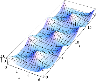
Figure 1: (color online). Plot of $n_{e}(x,t)$ when only $A_{1}=0.5$ is nonzero, and $\nu=\eta=10^{-5}$. This corresponds to $n_{0}=1.45\times 10^{18}$ m^-3 and $\lambda=4.32$ m, if we assume $T_{e}=10$ eV and $\lambda_{Q}/10=2$. Damping is practically invisible for the times presented.

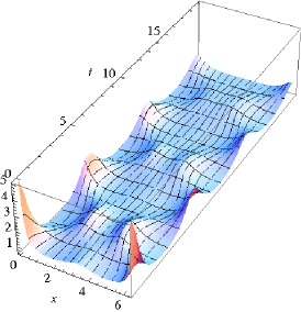
Figure 2: (color online). Plot of $n_{e}(x,t)$ when only $A_{1}=0.4$ and $A_{2}=0.2$ are nonzero, $\nu=0.02$ and $\eta=10^{-6}$. This corresponds to $n_{0}=1.45\times 10^{13}$ m^-3 and $\lambda=30.6$ m, if we assume $T_{e}=1$ eV and $\lambda_{Q}/10=2$. The viscous damping is evident after a single period.

In Figs. 1 and 2 we present typical examples for a small number of modes included. Various spatially periodic structures can be produced. Note the relevance of our considerations to a wide range of both laboratory and space plasmas.

The electron density $n_{e}(x,t)$ is an even and periodic function of $x$ with wavelength $2\pi$. It can be expanded in a Fourier series in $x$ with time dependent Fourier coefficients:

$$n_{e}(x,t)=1+\sum_{m=1}^{\infty}B_{m}(t)\cos(mx).$$ (23)

This along with the first equation in (20) integrated over $dx$ leads to the Fourier expansion of $E(x,t)$:

$$E(x,t)=-\sum_{m=1}^{\infty}\frac{B_{m}(t)}{m}\sin(mx).$$ (24)

And finally, Eqs. (13) and (24) lead to

$$n_{e}(x,t)v_{e}(x,t)=\frac{\partial E}{\partial t}=-\sum_{m=1}^{\infty}\frac{dB_{m}(t)}{dt}\frac{\sin(mx)}{m},$$ (25)

from which $v_{e}(x,t)$ can be determined.

The coefficients $A_{n}$ and $B_{m}(t)$ are related by

$$\begin{split}A_{n}&=-\frac{2}{n\pi}\int_{0}^{\pi}\cos\Bigl{\{}n\Bigl{[}x+\sum_{m=1}^{\infty}\frac{B_{m}(0)}{m}\sin(mx)\Bigr{]}\Bigr{\}}\,dx,\\ B_{m}(t)&=\frac{2}{\pi}\int_{0}^{\pi}\cos\Bigl{\{}m\Bigl{[}s-\sum_{n=1}^{\infty}A_{n}G_{n}(t)\sin(ns)\Bigr{]}\Bigr{\}}\,ds.\end{split}$$ (26)

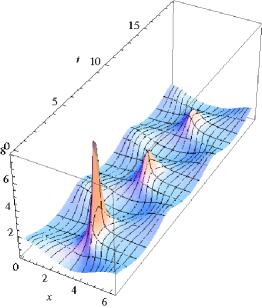
Figure 3: (color online). Plot of $n_{e}(x,t)$ when only $B_{1}(0)=0.55$ is nonzero, $\nu=0.015$, $\eta=10^{-5}$ and $N=20$. This corresponds to $n_{0}=1.45\times 10^{21}$ m^-3 and $\lambda=11.2\times 10^{-3}$ m, if we assume $T_{e}=100$ eV and $\lambda_{Q}/10=2$. Note that in the presence of even weak viscosity $B_{1}(0)$ can exceed $1/2$, see Eqs. (21).

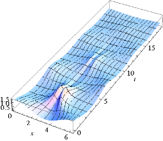
Figure 4: (color online). Plot of $n_{e}(x,t)$ when only $B_{1}(0)=0.55$ is nonzero, $\nu=0.1$ $\eta=10^{-4}$ and $N=20$. This corresponds to $n_{0}=1.45\times 10^{20}$ m^-3 and $\lambda=1.36\times 10^{-3}$ m, if we assume $T_{e}=10$ eV and $\lambda_{Q}/10=2$. The observed bifurcation of the maximum under strong viscosity is a new nonlinear effect.

These integrals are not expressible in terms of elementary functions, but if the sum over $m$ or $n$ is truncated at some $M$ or $N$, one can easily calculate numerically as many integrals as needed. If either $M=1$ or $N=1$, $A_{n}$ or $B_{m}(t)$ is expressible in terms of Bessel functions. Thus using the identity rizik (p. 185)

$$\int_{0}^{\pi}\cos(ax-z\sin x)\,dx=\pi J_{a}(z),$$ (27)

we obtain respectively

$$A_{n}=\frac{2}{n}(-1)^{n+1}J_{n}(nB_{1}(0))\quad\text{if }B_{m}(0)=0\text{ for }m>1,$$ (28)

$$B_{m}(t)=2J_{m}(mA_{1}G_{1}(t))\quad\text{if }A_{n}=0\text{ for }n>1.$$ (29)

Eqs. (26) result from standard formulas for Fourier coefficients, for the function $n_{e}(s,t=0)^{-1}$ or $n_{e}(x,t)$ as a function of $x$, if the integration variable in these formulas is changed from $s=x-E$ to $x$ ($n_{e}^{-1}\,ds=dx$) or conversely from $x=s+E$ to $s$ ($n_{e}\,dx=ds$), see Eqs. (21a) and (11).

Eqs. (29) and (23)–(25) present a new solution explicitly given in terms of physical variables $x$ and $t$. Its plot for $\nu=\eta=10^{-5}$ is shown in Fig. 1.

The particular solution (21) with $A_{n}$ given by (28) reduces to that of david if $\nu=\eta=0$ though in a different notation. The known condition $B_{1}(0)<1/2$ follows from the identity $\sum_{n=1}^{\infty}J_{n}(n\alpha)=\frac{\alpha}{2(1-\alpha)}$ rizik (p. 366). For $B_{1}(0)=1/2$, $n_{e}^{-1}$ becomes zero at $s=t=\pi$.

The behavior of this solution for $\nu,\eta>0$ is shown in Figs. 3 and 4. In a viscous and resistive plasma $B_{1}(0)$ can exceed $1/2$. Furthermore if $\nu$ is sufficiently large, see Fig. 4, where $\nu=0.1$, a new nonlinear effect can be noticed, i.e., the largest density maximum splits in two, with a saddle point between the peaks.

References

(1)
R. C. Davidson and P. P. Schram, Nuclear Fusion 8, 183
(1968); O. Buneman, Phys. Rev. 115, 503 (1959); J. M. Dawson, Phys.
Rev. 113, 383 (1959); R. C. Davidson, Methods in Nonlinear
Plasma Theory, (Academic, N. Y., 1972) Chap. 3.
(2) S. I. Braginski, in Voprosy Fiziki Plazmy, ed. by
M. A. Leontovitch, vol. 1 (Gosomizdat, Moscow, 1963);
P. C. Clemmow, J. P. Dougherty, Electrodynamics of
Particles and Fields, (Addison–Wesley, N. Y.,1990) Chap. 11.
(3) E. Infeld and G. Rowlands, Nonlinear Waves, Solitons
and Chaos, (2nd ed.) (Cambridge University Press, Cambridge, England, 2000)
Chap. 6; J. Tech. Phys. 28, 607 (1997) and 29, 3 (1998).
(4) I. M. Rizhik and I. S. Gradstein, Tables of Integrals
Sums Series and Products, (Gosizdat, Moscow, 1951).