Consistent Thermodynamics for Quasiparticle Boson System with Zero Chemical Potential

Abstract

The thermodynamic consistency of quasiparticle boson system with effective mass $m^{*}$ and zero chemical potential is studied. We take the quasiparticle gluon plasma model as a toy model. The failure of previous treatments based on traditional partial derivative is addressed. We show that a consistent thermodynamic treatment can be applied to such boson system provided that a new degree of freedom $m^{*}$ is introduced in the partial derivative calculation. A pressure modification term different from the vacuum contribution is derived based on the new independent variable $m^{*}$. A complete and self-consistent thermodynamic treatment for quasiparticle system, which can be widely applied to effective mass models, has been constructed.

I Introduction

System with complicated interaction is very common in real world and rich in physical phenomenon but very hard to deal with. In practise, physicists have introduced many theoretical tools, such as the Hartree-Fock approximation, approximate secondary quantization, summation of Feymann diagrams, etc., among which the quasiparticle approximation is one of the simplest first order approximation. Most of the quasiparticle approximations take the system as consisting of quasiparticles without interaction, while the effect of interaction is represented by the effective mass $m^{*}$, usually being a function of temperature $T$ and particle density $\rho$. It should be emphasized that the effective mass quasiparticle model is only a rough approximation since many detailed properties and higher order contributions are neglected. However, to some degree, it is still an efficient tool to discuss some macro properties of complex system because of its simplicity. The application of quasiparticle model to the study of thermodynamics can be found in many references, such as to the quark system Fowler:1981 ; Chakrabarty:1989 ; Chakrabarty:dual ; Benrenuto:1995dual ; Peng:1999 ; Wang:2000 ; Peng:2000 ; Zhang:2001 ; Zhang:dual ; Wen:2005 or quark-gluon plasma (QGP) Goloviznin:1993 ; Peshier:1994 ; YangShinNan:1995 ; Peshier:1996 ; Levai:1998 ; Schneider:2001 ; Biro:2003 ; Bannur:2007 .

However, it is well known that the effective mass quasiparticle model suffers from the thermodynamic inconsistency. To illustrate this inconsistency, for a quasiparticle boson system with chemical potential $\mu=0$, the standard expressions of pressure, $p=-\Omega/V=-\frac{gT}{2\pi^{2}}\int_{0}^{\infty}k^{2}\ln[1-\exp(-\epsilon/T)]dk$, and internal energy density, $\varepsilon=\frac{g}{2\pi^{2}}\int_{0}^{\infty}k^{2}\frac{\epsilon}{\exp(\epsilon/T)-1}dk$, will not satisfy some differential relations, such as $\varepsilon=T\frac{dp}{dT}-p$ YangShinNan:1995 . The problem comes from that the effective mass, being a function of medium parameters, entangles the usual thermodynamic relations via the relativistic dispersion relation $\epsilon(k)=\sqrt{k^{2}+m^{*2}(T,\rho)}$. As was shown in Ref.Yin:2008 , the usual thermodynamic treatment with traditional partial derivative to obtain the thermodynamic quantities is problematic. The reason is that the thermodynamic potential $\Omega$ of quasiparticle model is not only a function of characteristic variables $T$, $V$ and $\mu$, but also depends explicitly on the effective mass, $\Omega=\Omega(T,V,\mu,m^{*})$. To overcome this difficulty, there are many different treatments in the market. For example: (I). Calculate the derivatives of $m^{*}$ with respect to $T$ and $\rho$ in the differential relations for a reversible process,

$$d\Omega=-SdT-pdV-\overline{N}d\mu,$$ (1)

$$S=-\left(\frac{\partial\Omega}{\partial T}\right)_{V,\mu},\qquad p=-\left(\frac{\partial\Omega}{\partial V}\right)_{T,\mu},\qquad\overline{N}=-\left(\frac{\partial\Omega}{\partial\mu}\right)_{T,V},$$ (2)

where $S$, $p$ and $\overline{N}$ are entropy, pressure and average particle number, respectively. Many extra terms involving $\frac{\partial\Omega}{\partial m^{*}}\frac{\partial m^{*}}{\partial\rho}$ and $\frac{\partial\Omega}{\partial m^{*}}\frac{\partial m^{*}}{\partial T}$ will emerge in the expressions of $p$, $\varepsilon$ and entropy density $s$ Benrenuto:1995dual ; Peng:2000 ; Wen:2005 . But as was summarized in Ref.Yin:2008 , though many authors follow this direction, the extra terms in different references contradict each other. (II). Introduce a temperature- and/or density-dependent vacuum energy YangShinNan:1995 ; Biro:2003 ; Wang:2000 and force the vacuum to cancel the thermodynamic inconsistency. However, the physics of the vacuum is still unclear. (III). A new treatment had been suggested in our previous paper Yin:2008 . We introduce a new degree of freedom $m^{*}$ for the quasiparticle model effectively in the thermodynamic derivative relation and rewrite Eq.(1) as

$$d\Omega=-SdT-pdV-\overline{N}d\mu+Xdm^{*},$$ (3)

then Eq.(2) becomes

$$S=-\left(\frac{\partial\Omega}{\partial T}\right)_{V,\mu,m^{*}},\quad p=-\left(\frac{\partial\Omega}{\partial V}\right)_{T,\mu,m^{*}},\quad\overline{N}=-\left(\frac{\partial\Omega}{\partial\mu}\right)_{T,V,m^{*}},\quad X=\left(\frac{\partial\Omega}{\partial m^{*}}\right)_{T,V,\mu},$$ (4)

where $X$ is an extensive quantity corresponding to the intensive variable $m^{*}$. We emphasize that after introducing the term $Xdm^{*}$ in Eq.(3), we have Eq.(4) instead of Eq.(2). Since $m^{*}$ is an invariant in the partial derivatives for $S$, $p$ and $\overline{N}$, all the extra terms involving $\frac{\partial\Omega}{\partial m^{*}}\frac{\partial m^{*}}{\partial\rho}$ and $\frac{\partial\Omega}{\partial m^{*}}\frac{\partial m^{*}}{\partial T}$ are forbidden there. We have proven in Ref.Yin:2008 , by keeping $m^{*}$ invariant during the derivatives, the results remain self-consistent and in accord with the equilibrium statistics.

Noticing that at a fixed instant in the reversible process, the system is in an equilibrium state with temperature and density denoted as $T_{0}$ and $\rho_{0}$, respectively, then the effective mass of the quasiparticle becomes constant $m^{*}(T_{0},\rho_{0})\equiv m_{0}$. In this equilibrium state, the system reduces to a usual ideal gas system with constant particle mass $m_{0}$, whose thermodynamic quantities can be directly obtained statistically. In Ref.Yin:2008 we have proven that the thermodynamic quantities calculated in equilibrium state are just the corresponding quantities given by Eqs.(3) and (4). The introduction of the new variable $m^{*}$ can be understood in the following aspect. In the quasiparticle approximation, the effective mass summarizes the interaction, the confinement mechanism, etc., which must be reflected in a consistent thermodynamic treatment. It forces us to introduce $m^{*}$ as a new independent variable in the partial derivative to get a suitable treatment. Employing the quark mass density-dependent model, we had shown this treatment is thermodynamically self-consistent Yin:2008 . The ambiguities and inconsistencies in previous thermodynamic treatments are overcome.

The motivation of this paper is to extend our study from the fermion system to the boson system with non-conserved particles. The chemical potential $\mu$ equals zero for such system. We here take a quasiparticle gluon plasma (qGP) model, which was first introduced in Refs.Goloviznin:1993 ; Peshier:1994 , as a toy model to illustrate our treatment. This model is quite rough: On the one hand, it can not describe the properties of the real QGP exhibited by recent RHIC experiments Adams:2005 ; Adcox:2005 . One the other hand, one can calculate the hard thermal or dense loops Braaten:1990 ; Frenkel:1990 ; Blaizot:dual by temperature quantum theory and get higher order contributions beyond mean field and quasiparticle picture. However, we will still employ this model. The reasons are threefold: (1). The model is very simple and we can use this model to illustrate our treatment transparently. (2). This model has been employed by many authors to discuss the thermodynamic inconsistency in the physics market YangShinNan:1995 ; Biro:2003 ; Bannur:2007 . We use this model in favor of comparing our treatment with others. (3). This model has the lattice simulation results Engels:1989 ; Boyd:1995dual , which can be used as standards in comparing different treatments to expose their advantages and shortcomings. We will focus our attention to treatment (I) and treatment (III) since the study of qGP model by treatment (II) was shown in Ref.YangShinNan:1995 in detail. We will prove that the results given by traditional partial derivative treatment (I) are completely different from those of the lattice simulation. This treatment is failure for the qGP system as for the quark system Yin:2008 .

Another important problem involves the negative pressure. Of course, a real gluon plasma has no negative pressure. But as is predicted by lattice simulation, the QGP system experiences a phase transition at a critical temperature $T_{c}$ below which the system becomes comfined. One need to introduce the negative pressure at $T<T_{c}$ indicating the instability in the quasiparticle model to describe the phase transition at $T_{c}$. In treatment (I) Benrenuto:1995dual ; Peng:2000 ; Wen:2005 , the authors claimed that the term $\frac{\partial\Omega}{\partial m^{*}}\frac{\partial m^{*}}{\partial\rho}$ contributes a negative pressure which can cause the instability at low $T$. But unluckily, in Ref.Yin:2008 , we proved this term can not exist in a consistent treatment. In treatment (II), the authors obtained the negative pressure from the vacuum YangShinNan:1995 ; Biro:2003 ; Wang:2000 . In this paper, we will show that the negative pressure can exist naturally in treatment (III). It is not necessary to involve the vacuum. The newly independent variable $m^{*}$ permits a freedom for an arbitrary function $f(m^{*})$ in the formula of pressure, whose value can be determined by the comparison with experiment results or lattice data.

The paper is organized as follows: In the next section, using the lattice data as the criterion for comparison, we will examine the qGP model by treatment (I). In Sec. III, similar comparison will be made between the lattice data and our treatment (III). Then in Sec. IV, a modification term to pressure and entropy is derived within our self-consistent treatment (III). We will show this modification term is different from the vacuum contribution but a natural result of our newly introduced variable $m^{*}$. Sec. V is a brief summary.

II The results of treatment (I)

For the thermodynamic system with effective mass, after calculating the derivatives of $m^{*}$ to $T$ and $\rho$ in Eq.(2), one obtained Wen:2005

$$p = -\widetilde{\Omega}-V\frac{\partial\widetilde{\Omega}}{\partial V}+\rho\frac{\partial\widetilde{\Omega}}{\partial m^{*}}\frac{\partial m^{*}}{\partial\rho},$$ (5)

$$\varepsilon = \widetilde{\Omega}-\mu\frac{\partial\widetilde{\Omega}}{\partial\mu}-T\frac{\partial\widetilde{\Omega}}{\partial T}-T\frac{\partial\widetilde{\Omega}}{\partial m^{*}}\frac{\partial m^{*}}{\partial T},$$ (6)

$$s = -\frac{\partial\widetilde{\Omega}}{\partial T}-\frac{\partial\widetilde{\Omega}}{\partial m^{*}}\frac{\partial m^{*}}{\partial T},$$ (7)

where $\widetilde{\Omega}\equiv\Omega/V$ denotes the thermodynamic potential density. The qGP model is a perfect boson system with vanishing chemical potential $\mu$ and temperature- and density-dependent particle mass $m^{*}$, so the thermodynamic potential density

$$\widetilde{\Omega}=\frac{gT}{(2\pi)^{3}}\int\ln\left(1-e^{-\beta\sqrt{k^{2}+m^{*2}}}\right)dk^{3},$$ (8)

which is explicitly independent of $V$ for infinite qGP system. Eqs.(5) and (6) reduce to

$$p = -\widetilde{\Omega}+\rho\frac{\partial\widetilde{\Omega}}{\partial m^{*}}\frac{\partial m^{*}}{\partial\rho},$$ (9)

$$\varepsilon = \widetilde{\Omega}-T\frac{\partial\widetilde{\Omega}}{\partial T}-T\frac{\partial\widetilde{\Omega}}{\partial m^{*}}\frac{\partial m^{*}}{\partial T}.$$ (10)

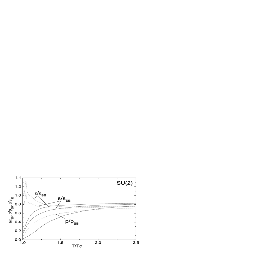
Figure 1: Internal energy density, pressure and entropy density as functions of temperature in SU(2) GP system. The solid curves are the lattice data from Ref.Engels:1989 ; while the dotted curves are the results of treatment (I).

Now we employ Eqs.(7-10) and three different models to study the properties of qGP model. The results are shown in Figs.1-3.

The first model is an SU(2) qGP model. The detail of this model has been addressed in Ref.YangShinNan:1995 and all the parameters including the fitting of $m^{*}$ which we used for calculation are from there. The results are shown in Fig.1, where the curves of energy density, pressure and entropy density are normalized to their Steven-Boltzmann limits, respectively. The solid curves adopted from Ref.Engels:1989 are given by the lattice QCD calculation which we use as the standard to compare different treatments. The dotted curves are the results of Eqs.(7-10). We see from Fig.1 that the deviation between solid curves and the corresponding dotted curves are remarkable, especially in low temperature regions.

The second and the third models are SU(3) qGP models. The details of these models have been addressed in Ref.Bannur:2007 , where the effective mass of SU(3) gluon is given by

$$m^{*2}=\frac{a_{0}\alpha_{s}(T)\rho}{T},\quad\textrm{model I},$$ (11)

and

$$m^{*2}=\frac{3a_{0}\alpha_{s}(T)\rho}{2T},\quad\textrm{model II},$$ (12)

where the constant $a_{0}=2.15$ and the two-loop order running coupling constant

$$\alpha_{s}(T)=\frac{2\pi}{11\ln(T/\Lambda_{T})}\left(1-\frac{51\ln(2\ln(T/\Lambda_{T}))}{121\ln(T/\Lambda_{T})}\right).$$ (13)

The only parameter $\lambda=\Lambda_{T}/T_{c}$ is fitted according to the lattice data as $\lambda=0.83$ for model I and $\lambda=0.7$ for model II. The results of treatment (I) are shown in Figs.2 and 3 for model I and model II, respectively. The inconsistency is transparently seen again. One can prove the deviation can not be conciliated by different choices of $\lambda$. From Figs.1-3, the failure of treatment (I) is obvious. The shapes of the curves are completely different.

III The results of treatment (III)

As demonstrated in our previous work Yin:2008 , the exact differential relations of thermodynamic functions in quasiparticle model should take the effective mass as a new independent degree of freedom. In grand canonical ensemble, the exact differential relation of $\Omega$ should be rewritten as Eqs.(3) and (4). We have proven that these formulae are self-consistent and agree with the statistical definitions and relations of thermodynamic quantities Yin:2008 . Employing Eq.(4), Eq.(8) and the energy definition

$$U=\sum_{i}g_{i}n_{i}\epsilon_{i}=\sum_{i}\frac{g_{i}\sqrt{m^{*2}+k_{i}^{2}}}{e^{\beta\sqrt{m^{*2}+k_{i}^{2}}}-1},\\$$ (14)

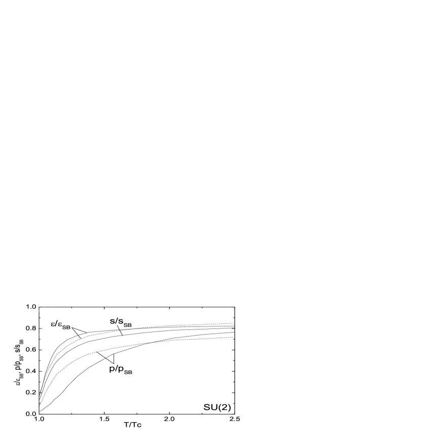
Figure 4: The same as Fig.1, except that the dashed curves are the results of treatment (III).

we calculate the corresponding thermodynamic quantities by treatment (III) for the SU(2) and SU(3) models in Sec. II. Our results are shown in Figs.4-6. In Fig.4, the solid curves and the dashed curves refer to the lattice data and the results of treatment (III) for the SU(2) model, respectively. The solid curve and dashed curve for the entropy density coincide since the function $m^{*}(T)$ are determined from the lattice data of entropy YangShinNan:1995 . Figs.5 and 6 are the same as those of Figs.2 and 3, except that the dashed curves are the results of our treatment (III). Comparing Figs.1-3 from treatment (I) with the corresponding Figs.4-6 from treatment (III), we see that the curves of our treatment (III) lies much closer to the lattice data, and the catastrophic deviation in Figs.1-3 disappears.

We are convinced by these results as well as Ref.Yin:2008 that treatment (I) with traditional partial derivative fails in the quasiparticle model with effective mass, and the thermodynamically consistent treatment (III), by introducing the new independent variable $m^{*}$ in the partial derivative calculation, produces much better results. However, treatment (III) in its present form can not give some expected properties. We see from Figs.5 and 6, the vanishing pressure at $T=T_{c}$ is exhibited by the lattice data, since below $T_{c}$ the system becomes confined and no free particle exists any more. But the present result of pressure of treatment (III) for quasiparticle model is always finitely positive at $T>0$. It is challenging to find a reasonable way to obtain a negative pressure modification to realize the phase transition at $T_{c}$ within our consistent treatment, this will be the topic in next section.

IV Modification to pressure and entropy without vacuum

Starting from the thermodynamic formula

$$\varepsilon+p-Ts=\frac{G}{V}=n\mu=0,$$ (15)

for qGP model and Eq.(4), we get

$$\varepsilon=T\left(\frac{\partial p}{\partial T}\right)_{m^{*}}-p=T^{2}\left(\frac{\partial(p/T)}{\partial T}\right)_{m^{*}},$$ (16)

The difference between Eq.(16) and its usual form, $\varepsilon=T\frac{dp}{dT}-p$, is significant. Instead of the total derivative $\frac{dp}{dT}$, we have the partial derivative with $m^{*}$ fixed, because $m^{*}$ is an independent variable in Eq.(3). We can integrate Eq.(16) and get

$$p=T\left[\int^{T}\frac{\varepsilon}{t^{2}}dt+f(m^{*})\right],$$ (17)

where $f(m^{*})$ is an arbitrary integral function of $m^{*}$. Eq.(17) shows the significant difference from the usual relation without taking $m^{*}$ as a free parameter. Obviously, if we choose $f(m^{*})=0$, Eq.(17) reduces to the normal ideal gas case.

According to Eq.(17), the thermodynamic potential $\Omega$, entropy $S$ and $X$ become

$$\Omega = -pV=-TV\int^{T}\frac{\varepsilon}{t^{2}}dt-TVf(m^{*}),$$ (18)

$$S = -\left(\frac{\partial\Omega}{\partial T}\right)_{V,m^{*}}=V\left[\frac{\varepsilon}{T}+\int^{T}\frac{\varepsilon}{t^{2}}dt+f(m^{*})\right],$$ (19)

$$X = \left(\frac{\partial\Omega}{\partial m^{*}}\right)_{T,V}=-TV\int^{T}\frac{1}{t^{2}}\left(\frac{\partial\varepsilon}{\partial m^{*}}\right)_{T,V}dt-TVf^{\prime}(m^{*}),$$ (20)

respectively. Then, noticing that $\mu=0$, the differential relation of internal energy $U$ reads

$$dU = d(\Omega+TS)$$ (21)

$$= TdS-pdV+Xdm^{*}$$

$$= Td\left\{V\left[\frac{\varepsilon}{T}+\int^{T}\frac{\varepsilon}{t^{2}}dt+f(m^{*})\right]\right\}-\left[T\int^{T}\frac{\varepsilon}{t^{2}}dt+Tf(m^{*})\right]dV$$

$$-\left[TV\int^{T}\frac{1}{t^{2}}\left(\frac{\partial\varepsilon}{\partial m^{*}}\right)_{T,V}dt+TVf^{\prime}(m^{*})\right]dm^{*}$$

$$= \left[\varepsilon+T\int^{T}\frac{\varepsilon}{t^{2}}dt+Tf(m^{*})\right]dV$$

$$+TV\left[\frac{d\varepsilon}{T}-\frac{\varepsilon}{T^{2}}dT+\frac{\varepsilon}{T^{2}}dT+\int^{T}\frac{1}{t^{2}}\left(\frac{\partial\varepsilon}{\partial m^{*}}\right)_{T,V}dm^{*}dt+f^{\prime}(m^{*})dm^{*}\right]$$

$$-\left[T\int^{T}\frac{\varepsilon}{t^{2}}dt+Tf(m^{*})\right]dV-TV\left[\int^{T}\frac{1}{t^{2}}\left(\frac{\partial\varepsilon}{\partial m^{*}}\right)_{T,V}dtdm^{*}+f^{\prime}(m^{*})dm^{*}\right]$$

$$= \varepsilon dV+Vd\varepsilon=d(V\varepsilon),$$

which means that $U$ is not affected by the arbitrary function $f(m^{*})$, and it still consists with the definition of internal energy in Eq.(14). This result is quite reasonable for the physical picture of the quasiparticle model. From Eqs. (17), (19) and (21), the relation

$$S=\frac{U+pV}{T}$$ (22)

remains correct.

Now we are in a position to determine $f(m^{*})$ from the lattice simulation data. Hereafter we choose the SU(3) model I and model II as our working examples, taking advantage of the clearly expressed $m^{*}$ in Eqs.(11) and (12).

With the effective mass in hand, the internal energy can be directly calculated from Eq.(14). For the pressure and entropy, one first calculate in equilibrium state as usual, the difference between the results and the lattice data gives the unknown function $f(m^{*})$, as is shown in Eqs.(18) and (19). But since the internal energy obtained by the given $m^{*}$ may generally different from the lattice data, remembering $U=TS-pV$ is satisfied by both the theoretical result and the data, the $f(m^{*})$ fitted from the pressure and the one from the entropy will be different, as was shown in Figs.7 and 8. Fig.7 refers to the SU(3) model I, where the dashed curve is for the $f(m^{*})/T^{3}$ fitted from the entropy data and the dotted curve for the one fitted from the pressure data, respectively. Fig.8 is the same as Fig.7 but for the SU(3) model II. We see from these two figures that the functions $f(m^{*})$ obtained from the lattice pressure data and the entropy data lie quite close to each other. With these results, the modified pressure and entropy density for these two models are shown in Figs.9 and 10, with the dotted line representing the entropy density modified by $f(m^{*})$ fitted from the pressure; and the dashed line representing the pressure modified by $f(m^{*})$ fitted from the entropy, respectively. We see from these two figures that the curves of modified pressure and entropy density agree with the lattice data quite well. The internal energy density is not changed due to Eq.(21), so it remains the same as in Figs.5 and 6 and is not plotted again in Figs.9 and 10. It is worth pointing out that if $m^{*}$ is not given previously but fitted by the internal energy from Eq.(14), the $f(m^{*})$ fitted from the pressure and the one from the entropy will be the same, and all the three curves will coincide exactly with the lattice data. In particular, the segments of negative pressure are plotted explicitly below $T_{c}$ in Figs.9 and 10. The function $f(m^{*})$ contributes the negative pressure in a natural fashion. The appearance of the negative pressure, unlike treatment (II) YangShinNan:1995 ; Biro:2003 ; Wang:2000 , does not relies on the vacuum. This is an important character of our treatment (III). At last, we would like to emphasize again that the negative pressure shown in Figs.9 and 10 at $T<T_{c}$ does not means such states really exist. In fact the quasiparticle model is only applicable for $T>T_{c}$. We keep the segments of the curves below $T_{c}$ just to demonstrate explicitly how the mechanism of negative pressure instability acts in the quasiparticle model within our treatment.

V Summary

With the qGP model as a toy model, we demonstrate explicitly again the difficulty of treatment (I) with traditional partial derivative and prove that our treatment (III) is applicable, by the criterion of the lattice data. We also demonstrate the success of the newly introduced function $f(m^{*})$ which can fit the lattice data self-consistently. It’s worth emphasizing that the physical meaning of the additional function is completely different from the vacuum energy. This function does not appear in the expression of $\varepsilon$, but change the values of $p$ and $s$. The basic differences between our treatment (III) and other treatments are as follows: (1). As was proven in Ref.Yin:2008 , treatment (III) is thermodynamically self-consistent and coincide with the statistics in equilibrium state. We do not need to introduce a vacuum and force it to cancel the thermodynamically inconsistent terms as in treatment (II). (2). We have an vacuum-unrelated integral function $f(m^{*})$ in the consistent treatment, which can be fixed by fitting to experiment data or standard theoretical results.

Together with our previous paper Yin:2008 , we have established a self-consistent and complete thermodynamics for the effective mass quasiparticle model. Our treatment (III) is not only applicable to fermion system with nonzero chemical potential, but also to boson system with zero chemical potential. It can be wildly applied in all quasiparticle system.

Figure 2: Internal energy density, pressure and entropy density as functions of temperature in SU(3) GP system with effective mass of model I and $\lambda=0.83$. The solid curves are the lattice simulation data from Ref.Boyd:1995dual , and dashed curves are the results of treatment (I).

Figure 3: The same as Fig.2, except that the effective mass is of model II, and $\lambda=0.7$.

Figure 5: The same as Fig.2, except that the dashed curves are the results of treatment (III).

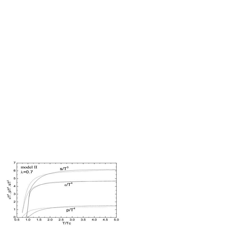
Figure 6: The same as Fig.3, except that the dashed curves are the results of treatment (III).

Figure 7: The modification term $f(m^{*})/T^{3}$ in SU(3) qGP model with $m^{*}$ of model I and $\lambda=0.83$.

Figure 8: The same as Fig.7, except that the effective mass is of model II and $\lambda=0.7$.

Figure 9: The same as Fig.5, but the pressure and entropy density are modified by $f(m^{*})$ in Fig.7.

Figure 10: The same as Fig.6, but the pressure and entropy density are modified by $f(m^{*})$ in Fig.8.

References

- (1) G. N. Fowler, S. Raha and R. M. Weiner, Z. Phys. C9, 271 (1981).
- (2) S. Chakrabarty, S. Raha, and B. Sinha, Phys. Lett. B229, 112 (1989).
- (3) S. Chakrabarty, Phys. Rev. D 43, 627 (1991); ibid. 48, 1409 (1993).
- (4) O. G. Benvenuto and G. Lugones, Phys. Rev. D 51, 1989 (1995); G. Lugones and O. G. Benvenuto, ibid. 52, 1276 (1995).
- (5) G. X. Peng, H. C. Chiang, P. Z. Ning, and B. S. Zou, Phys. Rev. C 59, 3452 (1999).
- (6) P. Wang, Phys. Rev. C 62, 015204 (2000).
- (7) G. X. Peng, H. C. Chiang, B. S. Zou, P. Z. Ning, and S. J. Luo, Phys. Rev. C 62, 025801 (2000).
- (8) Y. Zhang, R. K. Su, S. Q. Ying, and P. Wang, Europhys. Lett. 56, 361 (2001).
- (9) Y. Zhang and R. K. Su, Phys. Rev. C 65 035202 (2002); ibid. 67 015202 (2003).
- (10) X. J. Wen, X. H. Zhong, G. X. Peng, P. N. Shen, and P. Z. Ning, Phys. Rev. C 72, 015204 (2005).
- (11) V. Goloviznin and H. Satz, Z. Phys. C 57, 671 (1993).
- (12) A. Peshier, B. Kämpfer, O. P. Pavlenko, and G. Soff, Phys. Lett. B 337, 235 (1994).
- (13) M. I. Gorenstein and S. N. Yang, Phys. Rev. D 52, 5206 (1995).
- (14) A. Peshier, B. Kämpfer, O. P. Pavlenko, and G. Soff, Phys. Rev. D 54, 2399 (1996).
- (15) P. Lévai and U. Heinz, Phys. Rev. C 57, 1879 (1998).
- (16) R. A. Schneider and W. Weise, Phys. Rev. C 64, 055201 (2001).
- (17) T. S. Biró, A. A. Shanenko, and V. D. Toneev, Phys. Atom. Nucl. 66, 982 (2003).
- (18) V. M. Bannur, Phys. Lett. B647, 271 (2007); Phys. Rev. C 75, 044905 (2007).
- (19) S. Yin and R. K. Su, Phys. Rev. C 77, 055204 (2008).
- (20) J. Adams et al. [STAR Collaboration], Nucl. Phys. A757, 102 (2005).
- (21) K. Adcox et al. [PHENIX Collaboration], Nucl. Phys. A757, 184 (2005).
- (22) E. Braaten and R. D. Pisarski, Nucl. Phys. B337, 569 (1990).
- (23) J. Frenkel and J. C. Taylor, Nucl. Phys. B334, 199 (1990).
- (24) J. P. Blaizot, E. Iancu, and A. Rebhan, Phys. Rev. Lett. 83, 2906 (1999); Phys. Rev. D63, 065003 (2001).
- (25) J. Engels, J. Fingberg, K. Redlich, H. Satz, and M. Weber, Z. Phys. C 42, 341 (1989).
- (26) G. Boyd, J. Engels, F. Karsch, E. Laermann, C. Legeland, M. Lütgemeier, and B. Petersson, Phys. Rev. Lett. 75, 4169 (1995); Nucl. Phys. B469, 419 (1996).