On the Cramér-Rao Lower Bound for Frequency Correlation Matrices of Doubly Selective Fading Channels for OFDM Systems

Abstract

In this paper, the Cramér-Rao lower bound (CRLB) of the sample frequency correlation matrices (SFCM) is derived based on a rigorous model of the doubly selective fading channel for orthogonal frequency division multiplexing (OFDM) systems with pilot-symbol-aided modulation. By assuming a fixed pilot sequence and independent samples, SFCM is complex Wishart distributed. Then, the maximum likelihood estimator (MLE) and the exact expression of CRLB are obtained. From CRLB, the lower bounds of total mean squared error (TMSE) and average mean squared error (AvgMSE) independent of the pilot sequence are deduced, which reveal that the amount of samples is the dominant factor affecting AvgMSE while the signal-to-noise ratio and the maximum Doppler spread have negligible effect. Numerical simulations demonstrate the analytic results.

I Introduction

Playing a key role in the channel estimation for orthogonal frequency division multiplexing (OFDM) systems, the frequency correlation matrix (FCM) is utilized by many statistics-based channel estimation algorithms, e.g., the linear minimum mean-squared error (LMMSE) estimator and its optimal low-rank approximations [1], the MMSE estimator exploring both time and frequency correlations [2], the two-dimensional Wiener filtering [3], and those algorithms based on parametric channel model [4][5][6]. In real applications, the sample FCM (SFCM) is used in stead of the true one, and usually obtained through the least squared (LS) channel estimation.

For fixed or slowly moving radio channels whose Doppler spreads are relatively small, the channels reveal a feature of block-fading [7]. Hence, the Doppler spread affects the accumulation of SFCM negligibly. However, for fast moving radio channels, intra-symbol fading becomes so prominent that inter-carrier interference (ICI) takes effect by not only degrading the performance of OFDM systems [8], but also affecting the mean and covariance of SFCM. In [9], the bounds of the ICI power is derived.

The bias-property of SFCM in doubly selective fading channels has been investigated in [10]. As a counterpart, in this paper, we find out the Cramér-Rao lower bound (CRLB) for FCM to evaluate the performance of maximum likelihood estimator (MLE) and uncover the factors influencing the estimation accuracy.

This paper is organized as follows. In Section II, the OFDM system and channel model are introduced. Then, in Section III, CRLB for FCM is derived and further discussed to uncover the essential factors. Numerical results appear in Section IV. Finally, Section V concludes the paper.

Notation: Lowercase and uppercase boldface letters denote column vectors and matrices, respectively. $(\cdot)^{*}$, $(\cdot)^{H}$, and $||\cdot||_{F}$ denote conjugate, conjugate transposition, and Frobenius norm, respectively. $\otimes$ denotes the Kronecker product. $E(\cdot)$ represents expectation. $[{\bf{A}}]_{i,j}$ and $[{\bf{a}}]_{i}$ denotes the $(i$,$j)$-th element of ${\bf{A}}$ and the $i$-th element of ${\bf{a}}$, respectively. ${\text{diag}}({\bf{a}})$ is a diagonal matrix by placing ${\bf{a}}$ on the diagonal.

II System Model

Consider an OFDM system with a bandwidth of $BW=1/T$ Hz ($T$ is the sampling period). $N$ denotes the total number of tones, and a cyclic prefix (CP) of length $L_{cp}$ is inserted before each symbol to eliminate inter-block interference. Thus the whole symbol duration is $T_{s}=(N+L_{cp})T$.

The complex baseband model of a linear time-variant mobile channel with $L$ paths can be described by [11]

$${h(t,\tau)=\sum\limits_{l=1}^{L}{h_{l}(t)\delta\left({\tau-\tau_{l}T}\right)}}$$ (1)

where $\tau_{l}\in{\mathcal{R}}$ is the normalized non-sample-spaced delay of the $l$-th path, and $h_{l}(t)$ is the corresponding complex amplitude. According to the wide-sense stationary uncorrelated scattering (WSSUS) assumption, $h_{l}(t)$’s are modeled as uncorrelated narrowband complex Gaussian processes.

Furthermore, by assuming the uniform scattering environment introduced by Clarke [12], $h_{l}(t)$’s have the identical normalized time correlation function (TCF) for all $l$’s, thus the TCF of the $l$’s path is

$${r_{t,l}({\Delta}t)=\sigma_{l}^{2}J_{0}\left(2{\pi}{f_{d}}{\Delta}t\right)}$$ (2)

where $\sigma_{l}^{2}$ is the power of the $l$-th path, $f_{d}$ is the maximum Doppler spread, and $J_{0}(\cdot)$ is the zeroth order Bessel function of the first kind. Additionally we assume the power of channel is normalized, i.e., $\sum\nolimits_{l=0}^{L-1}\sigma_{l}^{2}=1$.

Assuming a sufficient CP, i.e., $L_{cp}\geq L$, the discrete signal model in the frequency domain is written as

$${\bf{y}}_{f}(n)={\bf{H}}_{f}(n){\bf{x}}_{f}(n)+{\bf{n}}_{f}(n)$$ (3)

where ${\bf{x}}_{f}(n),{\bf{y}}_{f}(n),{\bf{n}}_{f}(n)\in{\mathcal{C}}^{N\times 1}$ are the $n$-th transmitted and received signal and additive white Gaussian noise (AWGN) vectors, respectively, and ${\bf{H}}_{f}(m)\in{\mathcal{C}}^{N\times{N}}$ is the channel transfer matrix with the $(k+\nu,k)$-th element as

$$\left[{\bf{H}}_{f}(n)\right]_{k+\upsilon,k}=\frac{1}{N}\sum\limits_{m=0}^{N-1}\sum\limits_{l=1}^{L}h_{l}(n,m)e^{-j2{\pi}({\upsilon}m+k{\tau_{l}})/N}$$ (4)

where $h_{l}(n,m)=h_{l}(nT_{s}+(L_{cp}+m)T)$ is the sampled complex amplitude of the $l$-th path. $k$ and $\upsilon$ denote frequency and Doppler spread, respectively. Apparently, as ${\bf{H}}_{f}(n)$ is non-diagonal, ICI is present. In fact, when the normalized maximum Doppler spread $f_{d}T_{s}\leq 0.1$, the signal-to-interference ratio (SIR) is over 17.8 dB [13].

III CRLB for Frequency Correlation Matrices

Usually SFCM is obtained through the LS channel estimation. We consider OFDM systems adopting pilot-symbol-assisted modulation (PSAM) [1], hence only pilot symbols, denoted as ${\bf{y}}_{p}(n)\in\mathcal{C}^{N\times 1}$, are extracted and used to perform LS channel estimation. In addition, the pilot sequence is assumed to be invariant along the time. Therefore,

$${\bf{h}}_{p,ls}(n)={\bf{X}}_{p}^{-1}{\bf{y}}_{p}(n)={\bf{X}}_{p}^{-1}{\bf{H}}_{p}(n){\bf{x}}_{p}+{\bf{X}}_{p}^{-1}{\bf{n}}_{p}(n)$$ (5)

where ${\bf{X}}_{p}={\text{diag}}({\bf{x}}_{p})$ is a diagonal matrix consisting of pilot symbols, and the noise term is ${\bf{n}}_{p}(n)\sim{\mathcal{CN}}(0,\sigma_{n}^{2}{\bf{I}}_{N})$.

Denote the instantaneous channel impulse response (CIR) vector as ${\bf{h}}_{t}(n,m)=[h_{1}(n,m),\ldots,h_{L}(n,m)]^{T}$, $m=0,\ldots,N-1$, according to the assumptions of WSSUS and uniform scattering, ${\bf{h}}_{t}(n,m)$ is complex normal, i.e.,

$${\bf{h}}_{t}(n,m)\;{\sim}\;{\mathcal{CN}}_{L}(0,{\bf{D}})$$

where ${\bf{D}}={\text{diag}}({\sigma}_{l}^{2})$, $l=1,\ldots,L$. Then form the CIR matrix as ${\bf{H}}_{t}(n)=[{\bf{h}}_{t}(n,0),\ldots,{\bf{h}}_{t}(n,N-1)]$, so we have

$${\text{vec}}\left({\bf{H}}_{t}(n)\right)\;{\sim}\;{\mathcal{CN}}_{LN}(0,{\bf{\Omega}}\otimes{\bf{D}})$$

where ${\bf{\Omega}}\in{\mathcal{C}}^{N\times{N}}$ is a Toeplitz time correlation matrix (TCM), defined as

$$[{\bf{\Omega}}]_{m_{1},m_{2}}=J_{0}\left(2{\pi}{f_{d}}(m_{1}-m_{2})T\right)$$ (6)

Then according to (4), the channel transfer matrix ${\bf{H}}_{f}(n)={\bf{F}}_{\tau}{\bf{H}}_{t}(n)$, where ${\bf{F}}_{\tau}\in{\mathcal{C}}^{N\times{L}}$ is the unbalanced Fourier transform matrix, defined as $[{\bf{F}}_{\tau}]_{k,l}=e^{-j2{\pi}k{\tau}_{l}/N}$. Thus

$${\bf{H}}_{f}(n)\;{\sim}\;{\mathcal{CN}}_{N\times{N}}(0,{\bf{\Omega}}\otimes({\bf{F}}_{\tau}{\bf{D}}{\bf{F}}_{\tau}^{H}))$$ (7)

Assuming CIR is independent of the thermal noise, with (5) and (7), we have

$${\bf{h}}_{p,ls}(n)\;{\sim}\;{\mathcal{CN}}_{N}(0,{\bf{\Sigma}})$$ (8)

where the covariance matrix ${\bf{\Sigma}}$ is defined as

$${\bf{\Sigma}}=\omega{\bf{X}}_{p}^{-1}({\bf{R}}_{p}+\frac{{\sigma}_{n}^{2}}{\omega}{\bf{I}}_{N}){\bf{X}}_{p}^{-H}$$ (9)

where $\omega={\bf{x}}_{p}^{H}{\bf{\Omega}}{\bf{x}}_{p}$, and ${\bf{R}}_{p}={\bf{F}}_{\tau}{\bf{D}}{\bf{F}}_{\tau}^{H}$ is the true FCM.

When the LS estimated CFR’s, i.e., ${\bf{h}}_{p,ls}(n)$’s, are available, SFCM is constructed as

$${\bf{\hat{R}}}_{p,ls}=\frac{1}{N_{t}}\sum\limits_{n=1}^{N_{t}}{\bf{h}}_{p,ls}(n){\bf{h}}_{p,ls}^{H}(n)$$ (10)

where $N_{t}$ is the amount of samples. To derive the probability density function (PDF) of SFCM, we assume that samples are independent of each other, which may be a strict constraint. However, when the maximum Doppler spread is large and the spacing between two contiguous pilot symbols is comparatively small, the correlation between them is rather low, which alleviates the effect of model mismatch. Then, based on the assumption of independence and (8), we know that SFCM has the complex central Wishart distribution with $N_{t}$ degrees of freedom and covariance matrix ${\bf{\Sigma}}^{\prime}={\bf{\Sigma}}/N_{t}$ [14], denoted as

$${\bf{\hat{R}}}_{p,ls}\;{\sim}\;{\mathcal{CW}}_{N}(N_{t},{\bf{\Sigma}}^{\prime})$$ (11)

and its PDF is

$$f({\bf{\hat{R}}}_{p,ls})=\frac{{\text{etr}}(-{\bf{\Sigma}}^{\prime-1}{\bf{\hat{R}}}_{p,ls})(\det({\bf{\hat{R}}}_{p,ls}))^{N_{t}-N}}{{C\Gamma}_{N}(N_{t})(\det({\bf{\Sigma}}^{\prime})^{N_{t}}}$$ (12)

where ${\text{etr}}(\cdot)=\exp({\text{tr}}(\cdot))$ and ${C\Gamma}_{N}(N_{t})$ is the complex multivariate gamma function, defined as

$${C\Gamma}_{N}(N_{t})={\pi}^{N(N-1)/2}\prod\limits_{k=1}^{N}{\Gamma}(N_{t}-k+1)$$

Then, from (12), the likelihood function is written as

$${\text{L}}({\bf{R}}_{p}) = {\text{tr}}(-{\bf{\Sigma}}^{\prime-1}{\bf{\hat{R}}}_{p,ls})+(N_{t}-N)\ln(\det({\bf{\hat{R}}}_{p,ls}))$$

$$-\ln({C\Gamma}_{N}(N_{t}))-N_{t}\ln(\det({\bf{\Sigma}}^{\prime}))$$

Therefore, the score function with respect to the parameter matrix ${\bf{R}}_{p}$ is

$${\text{score}}({\bf{R}}_{p})=\frac{\partial{{\text{L}}({\bf{R}}_{p})}}{\partial{{\text{vec}}({\bf{R}}_{p})}}=\frac{\partial{{\text{vec}}({\bf{\Sigma}}^{\prime})^{T}}}{\partial{{\text{vec}}({\bf{R}}_{p})}}\times\frac{\partial{{\text{L}}({\bf{R}}_{p})}}{\partial{{\text{vec}}({\bf{\Sigma}}^{\prime})}}$$ (13)

where the first term on the right-hand side of (13) is

$$\frac{\partial{{\text{vec}}({\bf{\Sigma}}^{\prime})^{T}}}{\partial{{\text{vec}}({\bf{R}}_{p})}}=\frac{\omega}{N_{t}}({\bf{X}}_{p}^{-H}\otimes{\bf{X}}_{p}^{-1})$$ (14)

and the second term is

$$\frac{\partial{{\text{L}}({\bf{R}}_{p})}}{\partial{{\text{vec}}({\bf{\Sigma}}^{\prime})}}={\text{vec}}[({\bf{\Sigma}}^{\prime-1}{\bf{\hat{R}}}_{p,ls}{\bf{\Sigma}}^{\prime-1}-N_{t}{\bf{\Sigma}}^{\prime-1})^{T}]$$ (15)

By letting the score function equal zero and with (9), the MLE of FCM is derived as

$${\text{MLE}}({\bf{R}}_{p})=\frac{{\bf{X}}_{p}{\bf{\hat{R}}}_{p,ls}{\bf{X}}_{p}^{H}-{\sigma}_{n}^{2}{\bf{I}}_{N}}{{\bf{x}}_{p}^{H}{\bf{\Omega}}{\bf{x}}_{p}}$$ (16)

Note that (16) relies on the pre-known TCM, i.e., ${\bf{\Omega}}$, and noise power. For Rayleigh fading channels, it means the maximum Doppler spread, $f_{d}$, is known.

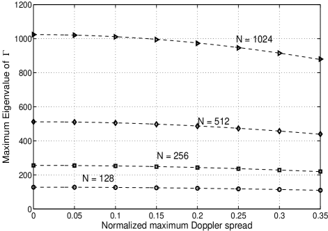
Figure 1: Fitting the maximum eigenvalues of ${\bf{\Omega}}$ with (27) for different sizes of FFT ($N$) and normalized Doppler’s ($f_{d}T_{s}$).

Further, according to the score function, the Fisher Information matrix with respect to ${\bf{R}}_{p}$ is

$${\bf{J}}({\bf{R}}_{p})=E\left[\left(\frac{\partial{{\text{L}}({\bf{R}}_{p})}}{\partial{{\text{vec}}({\bf{R}}_{p})}}\right)\left(\frac{\partial{{\text{L}}({\bf{R}}_{p})}}{\partial{{\text{vec}}({\bf{R}}_{p})}}\right)^{H}\right]$$ (17)

With (13)(14)(15), we have

$$\frac{\partial{{\text{L}}({\bf{R}}_{p})}}{\partial{{\text{vec}}({\bf{R}}_{p})}} = \frac{\omega}{N_{t}}({\bf{X}}_{p}^{-H}\otimes{\bf{X}}_{p}^{-1})$$

$$\times{\text{vec}}[({\bf{\Sigma}}^{\prime-1}{\bf{\hat{R}}}_{p,ls}{\bf{\Sigma}}^{\prime-1}-N_{t}{\bf{\Sigma}}^{\prime-1})^{T}]$$

so, (17) is rewritten into (18), shown at the bottom of the next page.

 

$${\bf{J}}({\bf{R}}_{p})=\frac{\omega^{2}}{N_{t}^{2}}({\bf{X}}_{p}^{-H}\otimes{\bf{X}}_{p}^{-1})E\{{\text{vec}}[({\bf{\Sigma}}^{\prime-1}{\bf{\hat{R}}}_{p,ls}{\bf{\Sigma}}^{\prime-1}-N_{t}{\bf{\Sigma}}^{\prime-1})^{T}]{\text{vec}}[({\bf{\Sigma}}^{\prime-1}{\bf{\hat{R}}}_{p,ls}{\bf{\Sigma}}^{\prime-1}-N_{t}{\bf{\Sigma}}^{\prime-1})^{T}]^{H}\}({\bf{X}}_{p}^{-H}\otimes{\bf{X}}_{p}^{-1})^{H}$$ (18)

Notice that

$${\bf{\Sigma}}^{\prime-1}{\bf{\hat{R}}}_{p,ls}{\bf{\Sigma}}^{\prime-1}\;{\sim}\;{\mathcal{CW}}_{N}(N_{t},{\bf{\Sigma}}^{\prime-1})$$

and

$$E[{\bf{\Sigma}}^{\prime-1}{\bf{\hat{R}}}_{p,ls}{\bf{\Sigma}}^{\prime-1}]=N_{t}{\bf{\Sigma}}^{\prime-1}$$

therefore

$$E\{{\text{vec}}[({\bf{\Sigma}}^{\prime-1}{\bf{\hat{R}}}_{p,ls}{\bf{\Sigma}}^{\prime-1}-N_{t}{\bf{\Sigma}}^{\prime-1})^{T}]$$ (19)

$$\;\;\;\;\;\;\;\;\;\;\;\;\times{\text{vec}}[({\bf{\Sigma}}^{\prime-1}{\bf{\hat{R}}}_{p,ls}{\bf{\Sigma}}^{\prime-1}-N_{t}{\bf{\Sigma}}^{\prime-1})^{T}]^{H}\}$$

$$= {\text{Var}}\{{\text{vec}}[({\bf{\Sigma}}^{\prime-1}{\bf{\hat{R}}}_{p,ls}{\bf{\Sigma}}^{\prime-1})^{T}]\}$$

Given ${\bf{S}}\sim{\mathcal{CW}}_{N}(N_{t},{\bf{\Sigma}}^{\prime})$, the entry of its second origin moment is [15]

$$E([{\bf{S}}]_{i,j}[{\bf{S}}]_{k,l})=N_{t}^{2}[{\bf{\Sigma}}^{\prime}]_{i,j}[{\bf{\Sigma}}^{\prime}]_{k,l}+N_{t}[{\bf{\Sigma}}^{\prime}]_{k,j}[{\bf{\Sigma}}^{\prime}]_{i,l}$$

Therefore, the entry of its second central moment is

$$E[([{\bf{S}}]_{i,j}-E([{\bf{S}}]_{i,j}))([{\bf{S}}]_{k,l}-E([{\bf{S}}]_{k,l}))]=N_{t}[{\bf{\Sigma}}^{\prime}]_{k,j}[{\bf{\Sigma}}^{\prime}]_{i,l}$$

Accordingly, (19) is rewritten as

$${\text{Var}}\{{\text{vec}}[({\bf{\Sigma}}^{\prime-1}{\bf{\hat{R}}}_{p,ls}{\bf{\Sigma}}^{\prime-1})^{T}]\}=N_{t}({\bf{\Sigma}}^{\prime-H}\otimes{\bf{\Sigma}}^{\prime-T})$$ (20)

Then, with (20), ${\bf{J}}({\bf{R}}_{p})$ is

$${\bf{J}}({\bf{R}}_{p})=\frac{\omega^{2}}{N_{t}}({\bf{X}}_{p}^{-H}\otimes{\bf{X}}_{p}^{-1})({\bf{\Sigma}}^{\prime-H}\otimes{\bf{\Sigma}}^{\prime-T})({\bf{X}}_{p}^{-1}\otimes{\bf{X}}_{p}^{-H})$$

From the Fisher Information matrix, the CRLB of ${\bf{R}}_{p}$ can be derived as [16][17]

$${\text{CRLB}}({\bf{R}}_{p}) = {\bf{J}}^{-1}({\bf{R}}_{p})$$ (21)

$$= \frac{N_{t}}{\omega^{2}}({\bf{X}}_{p}\otimes{\bf{X}}_{p}^{H})({\bf{\Sigma}}^{\prime H}\otimes{\bf{\Sigma}}^{\prime T})({\bf{X}}_{p}^{H}\otimes{\bf{X}}_{p})$$

$$= \frac{1}{N_{t}}(\frac{1}{\omega}{\bf{X}}_{p}{\bf{\Sigma}}^{H}{\bf{X}}_{p}^{H})\otimes(\frac{1}{\omega}{\bf{X}}_{p}^{H}{\bf{\Sigma}}^{T}{\bf{X}}_{p})$$

With (9), (21) can be further written as

$${\text{CRLB}}({\bf{R}}_{p})=\frac{1}{N_{t}}({\bf{R}}_{p}+\frac{{\sigma}_{n}^{2}}{\omega}{\bf{I}}_{N})\otimes({\bf{R}}_{p}+\frac{{\sigma}_{n}^{2}}{\omega}{\bf{I}}_{N})^{T}$$ (22)

Based on (22), a lower bound of the total mean squared error (TMSE) for ${\text{MLE}}({\bf{R}}_{p})$ is

$${\text{TMSE}}_{LB}({\bf{R}}_{p}) = {\text{tr}}({\text{CRLB}}({\bf{R}}_{p}))$$ (23)

$$= \frac{1}{N_{t}}{\text{tr}}^{2}({\bf{R}}_{p}+\frac{{\sigma}_{n}^{2}}{\omega}{\bf{I}}_{N})$$

$$= \frac{N^{2}}{N_{t}}(1+\frac{1}{\omega\gamma})^{2}$$

where $\gamma=\sigma_{n}^{-2}$ is the signal-to-noise ratio (SNR). And, accordingly, the lower bound of the average mean squared error (avgMSE) is

$${\text{AvgMSE}}_{LB}({\bf{R}}_{p})=\frac{{\text{TMSE}}_{LB}({\bf{R}}_{p})}{N^{2}}=\frac{1}{N_{t}}(1+\frac{1}{\omega\gamma})^{2}$$ (24)

(24) verifies the common sense that the more samples collected, the more accurate estimation acquired. And it also reveals that increasing SNR can reduce the estimation error. Furthermore, since

$${\omega}={\bf{x}}_{p}^{H}{\bf{\Omega}}{\bf{x}}_{p}=\|{\bf{x}}_{p}\|_{2}^{2}\times\frac{{\bf{x}}_{p}^{H}{\bf{\Omega}}{\bf{x}}_{p}}{{\bf{x}}_{p}^{H}{\bf{x}}_{p}}=\|{\bf{x}}_{p}\|_{2}^{2}\times{\text{R}}_{{\bf{x}}_{p}}({\bf{\Omega}})$$ (25)

where ${\text{R}}_{{\bf{x}}_{p}}({\bf{\Omega}})$ is the Rayleigh quotient of ${\bf{\Omega}}$ associated with the pilot sequence ${\bf{x}}_{p}$, and ${\text{R}}_{{\bf{x}}_{p}}({\bf{\Omega}})\leq{\lambda}_{max}$ where ${\lambda}_{max}$ is the maximum eigenvalue of ${\bf{\Omega}}$. Besides, when the power of pilot symbol is normalized, $\|{\bf{x}}_{p}\|_{2}^{2}=N$. Hence (24) is further lower bounded by

$${\overline{\text{AvgMSE}}}_{LB}({\bf{R}}_{p})=\frac{1}{N_{t}}(1+\frac{1}{N{\lambda}_{max}\gamma})^{2}$$ (26)

To further look into the relationship between $f_{d}T_{s}$ and ${\lambda}_{max}$, we examine the extreme eigenvalues of ${\bf{\Omega}}$ for different $f_{d}T_{s}$’s and $N$’s numerically, and the results are plotted in Fig.1. Moreover, we find a simple function fitting the maximum eigenvalues of all cases very well. The function is

$${\lambda}_{max}({\bf{\Omega}})=NJ_{0}(2{\pi}cf_{d}T_{s})$$ (27)

where $c=0.35$ when $f_{d}T_{s}\leq 0.35$. Therefore, a more insightful lower bound can be achieved by

$${\overline{\text{AvgMSE}}}_{LB}({\bf{R}}_{p})=\frac{1}{N_{t}}(1+\frac{1}{N^{2}J_{0}(2{\pi}{c}f_{d}T_{s})\gamma})^{2}$$ (28)

According to (28), we know that the amount of samples, i.e., $N_{t}$, effects the estimation accuracy dominantly but SNR and maximum Doppler spread do not, since $N^{2}$ is sufficiently large for most of current systems.

IV Numerical Results

The OFDM system in simulations is of $BW=1.25$ MHz ($T=1/BW=0.8$ ms), $N=128$, and $L_{cp}=16$. Two 3GPP E-UTRA channel models are adopted: Extended Vehicular A model (EVA) and Extended Typical Urban model (ETU) [18]. The excess tap delay of EVA is [$0$, $30$, $150$, $310$, $370$, $710$, $1090$, $1730$, $2510$] ns, and its relative power is [$0.0$, $-1.5$, $-1.4$, $-3.6$, $-0.6$, $-9.1$, $-7.0$, $-12.0$, $-16.9$] dB. For ETU, they are [$0$, $50$, $120$, $200$, $230$, $500$, $1600$, $2300$, $5000$] ns and [$-1.0$, $-1.0$, $-1.0$, $0.0$, $0.0$, $0.0$, $-3.0$, $-5.0$, $-7.0$] dB, respectively. The classic Doppler spectrum, i.e., Jakes’ spectrum [11], is applied to generate the Rayleigh fading channel.

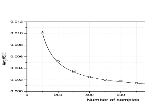
Figure 2: Comparison of analytic results (24) and numerical results for EVA and ETU channels when $\gamma=20$dB and $f_{d}=200$Hz.

In Fig.2, we compare the analytic results (24) and the numerical results over a range of $N_{t}$’s for EVA and ETU channels, respectively, when $\gamma=20$dB and $f_{d}=200$Hz. The pilot sequences are QPSK modulated and randomly chosen. And the collected samples are apart from each others far enough to guarantee the assumption of independence. Apparently, the analytic results meet the numerical ones quite well.

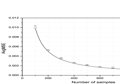
Figure 3: Comparison of analytic results (28) and numerical results for EVA and ETU channels when $\gamma=20$dB and $f_{d}=200$Hz.

In Fig.3, we compare the analytic results (28) and the numerical results for EVA and ETU channels, respectively, when $\gamma=20$dB and $f_{d}=200$Hz. The pilot sequences are QPSK modulated. In order to examine the effect of different pilot sequences on $\omega$, one hundred different sequences randomly generated are tested and their MSE’s are averaged and plotted. From the figure, we find that (28) is a tight bound even for an arbitrary pilot sequence.

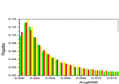
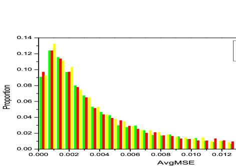
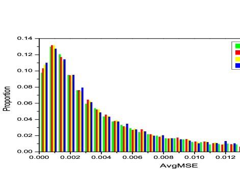
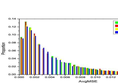
The distributions of avgMSE for different SNR’s and Doppler’s are plotted in Fig.4 through ten thousands estimations for EVA and ETU channels, respectively. The amount of samples of each test is 200, and the pilot sequences are QPSK modulated and randomly generated. Clearly, avgMSE’s are centered around zero and most of them are within the range of zero to CRLB, which follows that (16) is an unbiased estimator. Moreover, it is also obvious that the distributions of avgMSE for EVA and ETU channels are negligibly influenced by $\gamma$ and $f_{d}$, which follows the analytic lower bound (28).

V Conclusion

In this paper, the maximum likelihood estimator and CRLB of the frequency correlation matrix for OFDM systems in doubly selective fading channels are derived and analyzed. Through the analyses, we obtain an insightful lower bound of average MSE, i.e., (28), and according to which, the amount of samples shows a dominant impact on the accuracy of estimation while SNR and maximum Doppler spread have relatively small effect when the number of subcarriers are sufficiently large, although increasing SNR and decreasing maximum Doppler spread can help to reduce MSE slightly.

(a) EVA,$f_{d}=200$Hz.

(b) ETU,$f_{d}=200$Hz.

(c) EVA,$\gamma=15$dB.

(d) ETU,$\gamma=15$dB.

Figure 4: Distributions of average MSE for EVA and ETU channels when $N_{t}=200$.

References

• [1] O. Edfors, M. Sandell, J. van de Beek, S. Wilson, and P. Borjesson, “OFDM Channel Estimation by Singular Value Decompostion,” IEEE Trans. Commun., vol. 46, pp. 931–939, July 1998.
• [2] Y. Li, L. Cimini, and N. Sollenberger, “Robust Channel Estimation for OFDM Systems with Rapid Dispersive Fading Channels,” IEEE Trans. Commun., vol. 46, pp. 902–915, July 1998.
• [3] P. Hoeher, S. Kaiser, and P. Robertson, “Two-Dimensional Pilot-Symbol-Aided Channel Estimation by Wiener Filtering,” in IEEE ICASSP 1997, April 1997, pp. 1845–1848.
• [4] B. Yang et al., “Channel Estimation for OFDM Transmission in Multipath Fading Channels Based on Parametric Channel Modeling,” IEEE Trans. Commun., vol. 49, pp. 467–479, March 2001.
• [5] M. Raghavendra et al., “Parametric Channel Estimation for Pseudo-Random Tile-Allocation in Uplink OFDMA,” IEEE Trans. Signal Process., vol. 55, pp. 5370–5381, November 2007.
• [6] X. Zhao and T. Peng and W. Wang, “Parametric Channel Estimation by Exploiting Hopping Pilots in Uplink OFDMA,” in IEEE PIMRC 2008, Cannes, France, September 2008.
• [7] D. Shiu, G. Foschini, and M. Gans, “Fading Correlation and Its Effect on the Capacity of Multielement Antenna Systems,” IEEE Trans. Commun., vol. 48, pp. 502–513, March 2000.
• [8] T. Wang et al., “Performance Degradation of OFDM Systems Due to Doppler Spreading,” IEEE Trans. Wireless Commun., vol. 5, pp. 1422–1432, June 2006.
• [9] Y. Li and L. Cimini, “Bounds on the Interchannel Interference of OFDM in Time-Varying Impairments,” IEEE Trans. Commun., vol. 49, pp. 401–404, March 2001.
• [10] X. Zhao and M. Yang and T. Peng and W. Wang, “An Analysis of the Bias-Property of the Sample Auto-Correlation Matrices of Doubly Selective Fading Channels for OFDM systems,” Submitted to IEEE ICC 09, Dresden, Germany, June 2009.
• [11] R. Steele, Mobile Radio Communications.   IEEE Press, 1992.
• [12] R. Clarke, “A Statistical Theory of Mobile Radio Reception,” Bell Syst. Tech. J., pp. 957–1000, July-Auguest 1968.
• [13] Y. Choi, P. Voltz, and F. Cassara, “On Channel Estimation and Detection for Multicarrier Signals in Fast and Selective Rayleigh Fading Channels,” IEEE Trans. Commun., vol. 49, pp. 1375–1387, August 2001.
• [14] T. Ratnarajah, R. Vaillancourt, and M. Alvo, “Complex Random Matrices and Rayleigh Channel Capacity,” Commun. Inf. Syst., vol. 3, pp. 119–138, October 2003.
• [15] D. Maiwald and D. Kraus, “Calculation of Moments of Complex Wishart and Complex Inverse Wishart Distributed Matrices,” IEE Proc.-Radar. Sonar Navig., vol. 147, pp. 162–168, August 2000.
• [16] K. Mardia, J. Kent, and J. Bibby, Multivariate Analysis.   Academic Press, 1979.
• [17] G. Golub and C. V. Loan, Matrix Computations, 3rd ed.   New York: Johns Hopkins University Press, 1996.
• [18] “3GPP TS 36.101 v8.2.0 – Evolved Universal Terrestrial Radio Access (E-UTRA); User Equipment (UE) Radio Transmission and Reception (Relasase 8),” 3GPP, May 2008.