Doppler Spread Estimation by Subspace
Tracking for OFDM Systems

Abstract

In this paper, a novel maximum Doppler spread estimation algorithm is presented for OFDM systems with the comb-type pilot pattern. The least squared estimated channel frequency responses (CFR’s) on pilot tones are used to generate the auto-correlation matrices with/without a known lag, from which the time correlation function can be measured. The maximum Doppler spread is acquired by inverting the time correlation function. Since the noise term will bias the estimator, the estimated CFR’s are projected onto the delay subspace of the channel to reduce the bias term as well as the computation complexity. Furthermore, the subspace tracking algorithm is adopted to automatically update the delay subspace. Simulation results demonstrate the proposed algorithm can quickly converge to the true values for a wide range of SNR’s and Doppler spreads in Rayleigh fading channels.

I Introduction

In order to cope with various radio transmission scenarios, adaptive strategies, for example, adaptive modulation and coding and dynamic resource allocation, are widely employed by many orthogonal frequency division multiplexing (OFDM)-based wireless standards, e.g., TAB, TVB, IEEE 802.11/16 and 3GPP LTE [1]. Adaptive schemes automatically adjust the system configurations and transmission profiles according to some criteria to accommodate the varying radio environments.

The maximum Doppler spread is one of the key parameters of criteria for adaptive strategies. It determines the fading rate of the radio channel and its reciprocal is a metric of the coherent time of the channel. With the knowledge of it, wireless systems can change the depths of interleavers to reduce coding/decoding latencies, decrease unnecessary handoffs and adjust the rate of power control to reduce signalling overhead. More important, for OFDM systems, when the Doppler spread is comparable to the tone spacing, the orthogonality between tones would be corrupted, which would arise the inter-carrier interference (ICI) and consequently deteriorate the system performance. However, if the Doppler spread can be estimated, it will facilitate the adaptive schedule/control algorithms to appropriately tune systems to alleviate ICI.

Most of existing methods of estimating the maximum Doppler spread are categorized into two classes [2]: level crossing rate (LCR)-based and covariance (Cov)-based techniques. Since the algorithms reviewed in [2] were not specifically designed for OFDM systems, they did not exploit the special signal structure of OFDM systems. For OFDM systems, most literatures are Cov-based. [3] determined the maximum Doppler spread through estimating the smallest positive zero crossing point. In [4], Cai proposed to obtain the time auto-correlation function (TACF) in time domain by exploiting the cyclic prefix (CP) and its counterpart. However, Yucek [5] pointed out that for scalable OFDM systems whose CP sizes were varying over time, [4] was difficult to offer a sufficient estimation of TACF, which would degrade its estimation accuracy significantly. On the contrary, Yucek proposed to estimate the Doppler spread through the channel impulse responses (CIR’s) which were estimated from the periodically inserted training symbols.

Although the method in [5] seems to be more robust than in [4], its shortcomings are also evident. For example, in order to reduce system overheads, training symbols are arranged to be far from each other, and typically transmitted as preambles to facilitate the frame timing and carrier frequency synchronization. Once the duration of frame is longer than the coherent time of the channel, the maximum Doppler spread cannot be attained because TACF turns to irreversible. Moreover, for sparse training symbols, the converging speed of [5] would be very slow, which hinders its employment.

In this paper, we propose to estimate TACF by exploiting the comb-type pilot tones [6] which are widely adopted in wireless standards. In order to reduce noise perturbation, the estimated channel frequency responses (CFR’s) are projected onto the delay subspace [7] to obtain CIR’s, and the subspace tracking algorithm [8] is adopted as well to track the drifting delay subspace.

This paper is organized as follows. In Section II, the OFDM system and channel model are introduced. Then, the maximum Doppler spread estimation algorithm is presented in Section III. Simulation results and analyses are provided in Section IV. Finally, Section V concludes the paper.

II System Model

Consider an OFDM system with a bandwidth of $BW=1/T$ Hz ($T$ is the sampling period). $N$ denotes the total number of tones, and a CP of length $L_{cp}$ is inserted before each symbol to eliminate inter-block interference. Thus the whole symbol duration is $T_{s}=(N+L_{cp})T$. In each OFDM symbol, $P$ ($<N$) tones are used as pilots to assist channel estimation. In addition, optimal pilot pattern, i.e., equipowered and equispaced [9], is assumed. Pilot indexes are collected in the set ${\mathcal{I}}_{P}$, i.e., ${\mathcal{I}}_{P}=\{{\phi+p\times\theta}\}$, $(p=0,...,P-1)$, where $\phi$ and $\theta$ are the offset and interval, respectively.

The discrete complex baseband representation of a multipath CIR of length $L$ can be described by [10]

$${h(n,\tau)=\sum\limits_{l=0}^{L-1}{\gamma_{l}(n)\delta\left({\tau-\tau_{l}}\right)}}$$

where $\tau_{l}$ is the delay of the $l$-th path, normalized by the sampling period $T$, and $\gamma_{l}(n)$ is the corresponding complex amplitude. Due to the motion of users, $\gamma_{l}(n)$’s are wide-sense stationary (WSS) narrowband complex Gaussian processes, and uncorrelated with each other based on the assumption of uncorrelated scattering (US). In the sequel, $P\geq{L}$ and $P\times\theta=N$ are assumed for determinability and simplicity, respectively.

Furthermore, we assume the uniform scattering environment introduced by Clarke [11], thus $\gamma_{l}(n)$’s have the identical normalized TACF $J_{0}(2\pi{f_{d}}t)$ for all $l$’s, where $f_{d}$ is the maximum Doppler spread and $J_{0}(\cdot)$ is the zeroth order Bessel function of the first kind. Hence, the discrete TACF is

$${r_{t,l}(m)=\sigma_{l}^{2}J_{0}\left(2\pi|m|{f_{d}}T\right)}$$ (1)

where $\sigma_{l}^{2}$ is the power of the $l$-th path. Additionally we assume the power of channel is normalized, i.e., $\sum\nolimits_{l=0}^{L-1}\sigma_{l}^{2}=1$.

Assuming a sufficient CP, i.e., $L_{cp}\geq L$, the signal model in the time domain can be expressed as

$${y_{m}(n)=\sum\limits_{l=0}^{L-1}h_{m}(n,\tau_{l})x_{m}(n-\tau_{l})+w_{m}(n)}$$

where $x_{m}(n)$ and $y_{m}(n)$ are the $n$-th samples of the $m$-th transmitted and received OFDM symbols, respectively, $w_{m}(n)$ is the sample of additive white Gaussian noise (AWGN), i.e., $E[w_{m}(n)w_{m}^{*}(n+q)]=\sigma_{n}^{2}\delta(q)$, and $h_{m}(n,\tau_{l})$ is the corresponding sample of the time-varying CIR. Through some simple manipulations, the signal model in the frequency domain is written as

$${{\bf{Y}}_{m}={\bf{H}}_{m}{\bf{X}}_{m}+{\bf{W}}_{m}}$$ (2)

where ${\bf{X}}_{m},{\bf{Y}}_{m},{\bf{W}}_{m}\in\mathcal{C}^{N\times 1}$ are the $m$-th transmitted and received signal and noise vectors in the frequency domain, respectively, and ${\bf{H}}_{m}\in\mathcal{C}^{N\times{N}}$ is the channel transfer matrix whose $(\nu+k,k)$-th element, i.e., $[{\bf{H}}_{m}]_{\nu+k,k}$, is $\frac{1}{N}\sum\nolimits_{n=0}^{N-1}\sum\nolimits_{l=0}^{L-1}h_{m}(n,\tau_{l})e^{-j2\pi(\nu{n}+k\tau_{l})/N}$, where $k$ denotes subcarrier while $\nu$ denotes Doppler spread. Apparently, as ${\bf{H}}_{m}$ is non-diagonal, ICI is present. However, when the normalized maximum Doppler spread, i.e., $f_{d}T_{s}$, is less than 0.1, the signal-to-interference ratio (SIR) is over 17.8 dB [12], which enables us to discard non-diagonal elements of ${\bf{H}}_{m}$ with a negligible performance penalty.

As the comb-type pilot pattern is adopted, only pilot tones, denoted as ${\bf{Y}}_{P;m}\in\mathcal{C}^{P\times 1}$, are extracted from ${\bf{Y}}_{m}$. By approximating ${\bf{H}}_{m}$ to be diagonal, (2) is modified to

$${{\bf{Y}}_{P;m}={\bf{X}}_{P;m}{\bf{H}}_{P;m}+{\bf{W}}_{P;m}}$$ (3)

where ${\bf{X}}_{P;m}\in\mathcal{C}^{P\times{P}}$ is a pre-known diagonal matrix, and ${\bf{H}}_{P,m}\in\mathcal{C}^{P\times 1}$ consists of diagonal elements of ${\bf{H}}_{m}$. Hence, by denoting the instantaneous CFR as $H_{m}(n,k)=\sum\nolimits_{l=0}^{L-1}h_{m}(n,\tau_{l})e^{-j2\pi{k\tau_{l}}/N}$, we have $[{\bf{H}}_{P;m}]_{p}=\frac{1}{N}\sum\nolimits_{n=0}^{N-1}H_{m}(n,\phi+p\times\theta)$. Denote the Fourier transform matrix on the pilot tones as ${\bf{F}}_{P}\in\mathcal{C}^{P\times{N}}$, that is, $[{\bf{F}}_{P}]_{p,n}=\frac{1}{\sqrt{N}}e^{-j2\pi(\phi+p\times\theta)n/N}$, then ${\bf{W}}_{P;m}={\bf{F}}_{P}{\bf{w}}_{m}$, where ${\bf{w}}_{m}=[w_{m}(0),\ldots,w_{m}(N-1)]^{T}$, so, $E[{\bf{W}}_{P;m}{\bf{W}}_{P;m}^{H}]=\sigma_{n}^{2}{\bf{I}}_{P}$.

III Maximum Doppler Spread Estimation

At the receiver, the least-squared (LS) channel estimation on pilot tones is carried out firstly, i.e.,

$${{\bf{\hat{H}}}_{P;m}={\bf{X}}_{P;m}^{-1}{\bf{Y}}_{P;m}={\bf{H}}_{P;m}+{\bf{V}}_{P;m}}$$ (4)

where ${\bf{\hat{H}}}_{P;m}\in\mathcal{C}^{P\times 1}$ is the estimated CFR, and ${\bf{V}}_{P;m}\in\mathcal{C}^{P\times 1}$ is the noise vector expressed as ${{\bf{V}}_{P;m}={\bf{X}}_{P;m}^{-1}{\bf{W}}_{P;m}}$, hence, ${\bf{V}}_{P;m}\sim\mathcal{CN}(0,\sigma_{n}^{2}{\bf{I}}_{P})$ when ${\bf{X}}_{P;m}^{H}{\bf{X}}_{P;m}={\bf{I}}_{P}$ for PSK modulated pilot tones with equal power.

In the following, we will introduce a method of estimating the maximum Doppler spread based on TACF measured from significant paths of the channel obtained by projecting the LS estimated CFR onto the delay subspace.

III-A Measurement of the Time Auto-Correlation Function

First, by defining the Fourier transform matrix as ${\bf{F}}_{P,\tau}\in\mathcal{C}^{P\times{L}}$ with $[{\bf{F}}_{P,\tau}]_{p,l}=e^{-j2\pi(\phi+p\times\theta)\tau_{l}/N}$, ${\bf{H}}_{P;m}$ can be expressed as

$${\bf{H}}_{P;m}=\frac{1}{N}\sum\limits_{n=0}^{N-1}{\bf{H}}_{P;m}(n)=\frac{1}{N}\sum\limits_{n=0}^{N-1}{\bf{F}}_{P,\tau}{\bf{h}}_{m}(n)$$

where ${\bf{H}}_{P;m}$ and ${\bf{h}}_{m}(n)$ are CFR and instantaneous CIR vectors, respectively. Regardless of noise, the 0-lag auto-correlation matrix of ${\bf{H}}_{P;m}$ is

$${\bf{R}}_{{{\bf{H}}_{P}}}(0) = E\left[{\bf{H}}_{P;m}{\bf{H}}_{P;m}^{H}\right]$$ (5)

$$= \frac{1}{N^{2}}\sum\limits_{n=0}^{N-1}\sum\limits_{q=0}^{N-1}{\bf{F}}_{P,\tau}{\bf{A}}_{m}(n,q){\bf{F}}_{P,\tau}^{H}$$

where ${\bf{A}}_{m}(n,q)=E[{\bf{h}}_{m}(n){\bf{h}}_{m}^{H}(q)]$, and based on the assumption of WSSUS and Clarke model, its $(l_{1},l_{2})$-th element is $\left[{\bf{A}}_{m}(n,q)\right]_{l_{1},l_{2}}=\sigma_{l_{1}}^{2}r_{t}(n-q)\delta(l_{1}-l_{2})$, where $r_{t}(n)$ is the normalized TACF, hence ${\bf{A}}_{m}(n,q)$ is diagonal. Denoting ${\bf{D}}=diag(\sigma_{l}^{2})$, $l=0,\ldots,L-1$, we have

$${\bf{A}}_{m}(n,q)=r_{t}(n-q){\bf{D}}$$ (6)

Substitute (6) into (5) and with some manipulations

$${\bf{R}}_{{{\bf{H}}_{P}}}(0) = \xi(0){\bf{F}}_{P,\tau}{\bf{D}}{\bf{F}}_{P,\tau}^{H}$$ (7)

$$\xi(0) = \frac{1}{N^{2}}\sum\limits_{n=0}^{N-1}\sum\limits_{q=0}^{N-1}r_{t}(n-q)$$ (8)

Similarly, the $\beta$-lag auto-correlation matrix of ${\bf{H}}_{P;m}$ ($\beta\geq 0$), defined as ${\bf{R}}_{{{\bf{H}}_{P}}}(\beta)=E[{\bf{H}}_{P;m+\beta}{\bf{H}}_{P;m}^{H}]$, can be written as

$${\bf{R}}_{{{\bf{H}}_{P}}}(\beta) = \xi(\beta){\bf{F}}_{P,\tau}{\bf{D}}{\bf{F}}_{P,\tau}^{H}$$ (9)

$$\xi(\beta) = \frac{1}{N^{2}}\sum\limits_{n=0}^{N-1}\sum\limits_{q=0}^{N-1}r_{t}(n-q+(N+L_{cp})\beta)$$ (10)

Then, with (7) and (9), we have

$$\eta=\sqrt{\frac{||{\bf{R}}_{{\bf{H}}_{P}}(\beta)||_{F}^{2}}{||{\bf{R}}_{{\bf{H}}_{P}}(0)||_{F}^{2}}}=\frac{\xi(\beta)}{\xi(0)}$$ (11)

where $||{\cdot}||_{F}$ denotes the Frobenius norm. When the normalized Doppler spread $f_{d}T_{s}\leq 0.1$, referring to (1), we can make an approximation (which we will examine later) as

$$\eta\;\approx\;J_{0}(2\pi\beta(N+L_{cp})f_{d}T)$$ (12)

Since when $\beta(N+L_{cp})f_{d}T=\beta f_{d}T_{s}\leq 0.38$, $J_{0}(\cdot)$ is positive and reversible, meanwhile, in order to hold the orthogonality between subcarriers, $f_{d}T_{s}$ is usually smaller than 0.1, thus $\beta\leq 3$ is the feasible range. Then $f_{d}$ can be estimated by

$$\hat{f_{d}}=\frac{J_{0}^{-1}(\eta)}{2\pi\beta{T_{s}}}$$ (13)

Now we consider the effect of noise. When noise is present, (7) and (9) are rewritten into

$${\bf{\hat{R}}}_{{{\bf{H}}_{P}}}(0) = \xi(0){\bf{F}}_{P,\tau}{\bf{D}}{\bf{F}}_{P,\tau}^{H}+\sigma_{n}^{2}{\bf{I}}_{P}$$ (14)

$${\bf{\hat{R}}}_{{{\bf{H}}_{P}}}(\beta) = \xi(\beta){\bf{F}}_{P,\tau}{\bf{D}}{\bf{F}}_{P,\tau}^{H}$$ (15)

Correspondingly, (11) changes into

$$\eta=\sqrt{\frac{||{\bf{\hat{R}}}_{{\bf{H}}_{P}}(\beta)||_{F}^{2}}{||{\bf{\hat{R}}}_{{\bf{H}}_{P}}(0)||_{F}^{2}}}=\sqrt{\frac{\xi(\beta)^{2}}{\xi(0)^{2}+\rho^{2}}}$$ (16)

where $\rho$ is defined as

$$\rho=\sqrt{\frac{P\sigma_{n}^{4}}{||{\bf{F}}_{P,\tau}{\bf{D}}{\bf{F}}_{P,\tau}^{H}||_{F}^{2}}}$$ (17)

As pilot tones are equispaced, ${\bf{F}}_{P,\tau}^{H}{\bf{F}}_{P,\tau}=P{\bf{I}}_{L}$, then

$$||{\bf{F}}_{P,\tau}{\bf{D}}{\bf{F}}_{P,\tau}^{H}||_{F}^{2}=P^{2}\sum\limits_{l=0}^{L-1}\sigma_{l}^{4}$$

therefore, (17) is

$$\rho=\sqrt{\frac{\sigma_{n}^{4}}{P\sum\nolimits_{l=0}^{L-1}\sigma_{l}^{4}}}$$ (18)

Note $\sum\nolimits_{l=0}^{L-1}\sigma_{l}^{4}\leq(\sum\nolimits_{l=0}^{L-1}\sigma_{l}^{2})^{2}$, we have

$$\rho\geq\frac{1}{\sqrt{P}\times{SNR}}$$ (19)

where $SNR=\sigma_{n}^{-2}$ for the normalized power of the channel and pilot tones.

III-B Improving the Estimation Accuracy by the Delay Space

Although the maximum Doppler spread can be evaluated from (16) and (13), the effect of noise will bias the result of estimation heavily when $P$ is small and SNR is low. On the other hand, when $P$ is large, the effect of noise is negligible, but the sizes of ${\bf{\hat{R}}}_{{\bf{H}}_{P}}(0)$ and ${\bf{\hat{R}}}_{{\bf{H}}_{P}}(\beta)$ turn to be so large that evaluating their Frobenius norms would require a large amount of calculations, which hinders the employment of this method in real applications. Therefore, we introduce the delay subspace onto which the auto-correlation matrices are projected to reduce the effect of noise as well as the computation complexity.

Firstly, the eigenvalue decomposition (EVD) is performed

$${\bf{\hat{R}}}_{{{\bf{H}}_{P}}}(0) = {\bf{U}}_{\tau}\left[\xi(0){\bf{\Lambda}}+\sigma_{n}^{2}{\bf{I}}_{P}\right]{\bf{U}}_{\tau}^{H}$$ (20)

$${\bf{\hat{R}}}_{{{\bf{H}}_{P}}}(\beta) = {\bf{U}}_{\tau}\left[\xi(\beta){\bf{\Lambda}}\right]{\bf{U}}_{\tau}^{H}$$ (21)

Since the number of channel taps is $L$, $rank({\bf{\Lambda}})=L\leq{P}$, the last $P-L$ eigenvalues of ${\bf{\hat{R}}}_{{{\bf{H}}_{P}}}(0)$ and ${\bf{\hat{R}}}_{{{\bf{H}}_{P}}}(\beta)$ are $\sigma_{n}^{2}$ and 0, respectively. Once $L$ is available, ${\bf{U}}_{\tau}$ can be divided into two parts named as the ”signal” and ”noise” subspaces, respectively, i.e., ${\bf{U}}_{\tau}=[{\bf{U}}_{\tau,s},{\bf{U}}_{\tau,n}]$, where ${\bf{U}}_{\tau,s}\in\mathcal{C}^{P\times{L}}$, and so does ${\bf{\Lambda}}$, i.e., ${\bf{\Lambda}}=diag({\bf{\Lambda}}_{s},{\bf{0}}_{P-L})$, where ${\bf{\Lambda}}_{s}\in\mathcal{C}^{L\times{L}}$. Hence,

$${\bf{U}}_{\tau,s}^{H}{\bf{\hat{R}}}_{{{\bf{H}}_{P}}}(0){\bf{U}}_{\tau,s} = \xi(0){\bf{\Lambda}}_{s}+\sigma_{n}^{2}{\bf{I}}_{L}$$ (22)

$${\bf{U}}_{\tau,s}^{H}{\bf{\hat{R}}}_{{{\bf{H}}_{P}}}(\beta){\bf{U}}_{\tau,s} = \xi(\beta){\bf{\Lambda}}_{s}$$ (23)

Based on (22) and (23), (16) can be refined as

$$\eta=\sqrt{\frac{||{\bf{U}}_{\tau,s}^{H}{\bf{\hat{R}}}_{{{\bf{H}}_{P}}}(\beta){\bf{U}}_{\tau,s}||_{F}^{2}}{||{\bf{U}}_{\tau,s}^{H}{\bf{\hat{R}}}_{{{\bf{H}}_{P}}}(0){\bf{U}}_{\tau,s}||_{F}^{2}}}=\sqrt{\frac{\xi(\beta)^{2}}{\xi(0)^{2}+\rho_{r}^{2}}}$$ (24)

where $\rho_{r}$ is defined as

$$\rho_{r}=\sqrt{\frac{L\sigma_{n}^{4}}{||{\bf{\Lambda}}_{s}||_{F}^{2}}}$$ (25)

From (14)(15)(20)(21),

$$||{\bf{F}}_{P,\tau}{\bf{D}}{\bf{F}}_{P,\tau}^{H}||_{F}^{2}=||{\bf{\Lambda}}_{s}||_{F}^{2}$$

Hence, comparing (25) with (17), the bias term is reduced because

$$\frac{\rho_{r}}{\rho}=\sqrt{\frac{L}{P}}\leq 1$$ (26)

Actually, in the real circumstance, the number of significant taps of wireless channels is far less than of pilot tones, thereby projecting auto-correlation matrices onto the delay subspace, like (22) and (23), can effectively reduce the bias term and ease the calculation of $\eta$.

III-C Tracking the Delay Subspace – the Proposed Algorithm

When the user is moving, the tap delays of the channel, i.e., $\tau_{l}$’s, are slowly drifting [13][7], which causes ${\bf{F}}_{P;\tau}$ to vary and so does ${\bf{U}}_{\tau,s}$. To accommodate this variation, the subspace tracking algorithm is adopted to automatically update the delay subspace. In addition, if the number of significant taps of the channel is unknown, minimum description length (MDL) [14] is employed to estimate it. The proposed algorithm is summarized as follows.

  Initialize: ($n=0$) Q_0(0)  =Q_β(0)  =[I_L_m,0_L_m,P-L_m^T]^TA_0(0)  =A_β(0)  =0_P,L_mC_0(0)  =C_β(0)  =I_L_m

  Run: ($n=n+1$)Input: ${\bf{\hat{H}}}_{P}(n)$1) Updating for the 0-lag auto-correlation matrix:Z_0(n)  =Q_0(n-1)^H_P(n)A_0(n)  =αA_0(n-1)C_0(n-1)+(1-α)^H_P(n)Z_0(n)^HA_0(n)  =Q_0(n)R_0(n) : QR-factorizationC_0(n)  =Q_0(n-1)^HQ_0(n)^L(n)  =MDL(diag(R_0(n))) 2) Updating for the $\beta$-lag auto-correlation matrix:Z_β(n)  =Q_β(n-1)^H_P(n-β)A_β(n)  =αA_β(n-1)C_β(n-1)+(1-α)^H_P(n)Z_β(n)^HA_β(n)  =Q_β(n)R_β(n) : QR-factorizationC_β(n)  =Q_β(n-1)^HQ_β(n) 3) Estimating $\eta$ according to (24):

$$\hat{\eta}=\sqrt{\frac{\sum\nolimits_{l=1}^{{\hat{L}}(n)}|\left[{\bf{R}}_{\beta}(n)\right]_{l,l}|^{2}}{\sum\nolimits_{l=1}^{{\hat{L}}(n)}|\left[{\bf{R}}_{0}(n)\right]_{l,l}|^{2}}}$$

4) Estimating $f_{d}$ according to (13).

  Remark: $\alpha$ is a positive exponential forgetting factor close to 1. $L_{m}$ is the maximum rank to be tested. $MDL(\cdot)$ denotes the MDL detector and $diag({\bf{R}})$ denotes the diagonal elements of ${\bf{R}}$. In the simulation, we set $\alpha=0.995$ and $L_{m}=10$.

III-D Other Considerations

In this subsection, several further discussions about the proposed algorithm are presented.

First, numerical results are shown in Table I to examine (12) when $N=512$, $L_{cp}=64$ and $\beta=1$. From Table I, we find (12) is a good approximation when $\beta{f_{d}T_{s}}$ is small. It is worth noting that ${J_{0}(2\pi\beta{f_{d}}T_{s})}\leq{\eta}$, hence $f_{d}\geq\frac{J_{0}^{-1}(\eta)}{2\pi\beta{T_{s}}}$, in other words, (12) tends to over-estimate the maximum Doppler spread a bit.

TABLE I: A Table of Values of (12)

$f_{d}T_{s}$	0.02	0.04	0.06	0.08
$J_{0}(2\pi\beta{f_{d}}T_{s})$	0.9961	0.9843	0.9648	0.9378
$\eta\left(=\frac{\xi(\beta)}{\xi(0)}\right)$	0.9961	0.9843	0.9649	0.9381
$\frac{J_{0}(2\pi\beta{f_{d}}T_{s})}{\eta}$	1.0000	1.0000	0.9999	0.9997

Then we compare the computation complexity of the proposed algorithm with (16). The computation complexity of the subspace tracking is $\mathcal{O}(P\times{L}^{2})$ [8]. Since it takes a dominant proportion of the total number of instructions required by the proposed algorithm, we use it instead. Meanwhile, the computation complexity of (16), which directly computes the Frobenius norm of $P\times{P}$ matrices, is $\mathcal{O}(P^{2})$. Apparently, when $P>{L}^{2}$, which is usually the case for sparse multipath channels, the proposed algorithm can reduce the computation complexity considerably.

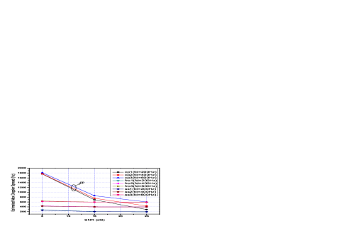
Figure 1: Performance comparison for the CP-based [4], Frobenius-norm-based (16) and subspace-based (24) algorithms when a 20ms frame is used and $\beta=1$.

IV Simulation Results

The performance of the proposed algorithm is evaluated for an OFDM system with $BW=5$ MHz ($T=1/BW=200$ ns), $N=512$, $L_{cp}=64$ and $P=64$. ITU Vehicular A Channels [15] is adopted, which consists of six individually faded taps with relative delays as $[0,310,710,1090,1730,2510]$ ns and average power as $[0,-1,-9,-10,-15,-20]$ dB. The classic Doppler spectrum, i.e., Jakes’ spectrum [10], is applied to generate the Rayleigh fading channel.

In Fig.1, a CP-based algorithm reported in [4] and (16), which is based on the Frobenius norm, are compared with the proposed subspace-based algorithm (24) with $\beta=1$. A 20ms frame including 194 OFDM symbols is used to generate the statistics. $f_{d}=200$, $400$ and $600$ Hz are tested under a range of SNR’s, respectively. Apparently, the CP-based algorithm fails for all $f_{d}$’s when the SNR is below 20 dB, meanwhile (16) and (24) work very well for all $f_{d}$’s and SNR’s but with a moderate positive bias for $SNR=5$ dB. In fact, when $SNR=5$ dB, resorting to (19) and (26), the lower bound of the bias terms $\rho$ and $\rho_{r}$ are 0.0395 for (16) and 0.0099 for (24), respectively. And when $f_{d}=600$ Hz, according to (8) and (10), $\xi(0)=0.9938$ and $\xi(\beta)=0.9476$. Thus, the relative errors of $\eta$ are 0.0007 and 0.0000 for (16) and (24), respectively, which almost have no effect on the estimation of the maximum Doppler spread. Therefore, (16) and (24) show almost the same performance when SNR’s are above 5 dB.

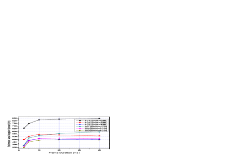
Figure 2: Performance comparison between the Frobenius-norm-based (16) and subspace-based (24) algorithms when $f_{d}=400$ Hz and $\beta=1$.

Fig.2 shows the performance comparison between the Frobenus-norm-based (16) and subspace-based (24) in the low SNR regime, specifically, below 5 dB, to emphasize the capability of noise depression of the latter. Different frame durations are used to obtain TACF. From the figure we can find (24) outperforms (16) for all the SNR’s and frame durations, although both of them over-estimate the maximum Doppler spread due to the non-negligible noise bias term in the low SNR regime, which is also the reason why increasing the length of observation record does not help to decrease the bias in this regime.

The convergence of the proposed subspace-tracking-based algorithm is shown in Fig.3. Three different maximum Doppler spreads are tested, i.e., $f_{d}=200$, $400$ and $600$ Hz, when $SNR=15$ dB. The curves are plotted from the thirtieth OFDM symbol. It is observed from the plot that all the three curves converge to their true values after numbers of OFDM symbols and, further, the higher the Doppler spread is, the faster the curve converges. This is due to the subspace is updating faster when the Doppler spread is higher. In addition, after converging, the estimated maximum Doppler spread is fluctuating around its true value in a small range, hence additional time-averaging can be employed to smooth the curve.

V Conclusions

In this paper, we propose a subspace-tracking-based maximum Doppler spread estimation algorithm which is applicable to OFDM systems with the comb-type pilot pattern. It enjoys three main advantages: i) alleviating the noise term; ii) reducing the computation complexity; iii) tracking the drifting delay subspace. Through simulations, the performance of the proposed algorithm is demonstrated to outperform the CP-based algorithm [4]. Moreover, since the proposed algorithm is based on the subspace tracking, it can be easily integrated into the channel estimator equipped with the subspace tracker [7][16], which lends a broad application promise to it.

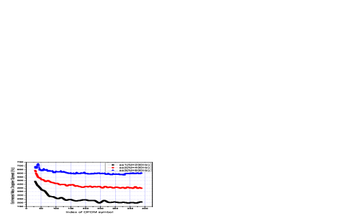
Figure 3: The convergence of the proposed subspace-tracking-based algorithm when $SNR=15$ dB and $\beta=1$.

References

- [1] H. Ekstrom, A. Furuskar et al., “Technical Solution for the 3G Long-Term Evolution,” IEEE Commun. Mag., pp. 38–45, March 2006.
- [2] C. Tepedelenlioglu, A. Abdi, G. Giannakis, and M. Kaveh, “Estimation of Doppler Spread and Signal Strength in Mobile Communications with Applications to Handoff and Adaptive Transmission,” Wirel. Commun. Mob. Comput., vol. 1, pp. 221–242, August 2001.
- [3] H. Schober and F. Jondral, “Velocity Estimation for OFDM Based Communication Systems,” in IEEE VTC-Fall 2002, vol. 2, Vancouver, BC, Canada, 2002, pp. 715–718.
- [4] J. Cai, W. Song, and Z. Li, “Doppler Spread Estimation for Mobile OFDM Systems in Rayleigh Fading Channels,” IEEE Trans. Consum. Electron., vol. 49, pp. 973–977, November 2003.
- [5] T. Yucek, R. Tannious, and H. Arslan, “Doppler Spread Estimation for Wireless OFDM Systems,” in IEEE/Sarnoff Symposium on Advances in Wired and Wireless Communication, 2005, pp. 233–236.
- [6] S. Coleri, M. Ergen, A. Puri, and A. Bahai, “Channel Estimation Techniques Based on Pilot Arrangement in OFDM Systems,” vol. 48, pp. 223–229, September 2002.
- [7] O. Simeone, Y. Bar-Ness, and U. Spagnolini, “Pilot-Based Channel Estimation for OFDM Systems by Tracking the Delay-Subspace,” vol. 3, pp. 315–325, January 2004.
- [8] P. Strobach, “Low-Rank Adaptive Filters,” IEEE Trans. Signal Process., vol. 44, pp. 2932–2947, December 1996.
- [9] S. Ohno and G. Giannakis, “Capacity Maximizing MMSE-Optimal Pilots for Wireless OFDM Over Frequency-Selective Block Rayleigh-Fading Channels,” IEEE Trans. Inf. Theory, vol. 50, pp. 2138–2145, September 2004.
- [10] R. Steele, Mobile Radio Communications. IEEE Press, 1992.
- [11] R. Clarke, “A Statistical Theory of Mobile Radio Reception,” Bell Syst. Tech. J., pp. 957–1000, July-Auguest 1968.
- [12] Y. Choi, P. Voltz, and F. Cassara, “On Channel Estimation and Detection for Multicarrier Signals in Fast and Selective Rayleigh Fading Channels,” IEEE Trans. Commun., vol. 49, pp. 1375–1387, August 2001.
- [13] D. Tse and P. Viswanath, Fundamentals of Wireless Communication. New York: Cambridge University Press, 2005.
- [14] M. Wax and T. Kailath, “Detection of Signals by Information Theoretic Criteria,” IEEE Trans. Acoust., Speech, Signal Process., vol. 33, pp. 387–392, April 1985.
- [15] “Guidelines for Evaluation of Radio Transmission Technologies for IMT-2000,” Recommendations ITU-R M.1225, 1997.
- [16] M. Raghavendra, E. Lior, S. Bhashyam, and K. Giridhar, “Parametric Channel Estimation for Pseudo-Random Tile-Allocation in Uplink OFDMA,” IEEE Trans. Signal Process., vol. 55, pp. 5370–5381, November 2007.