Parametric Channel Estimation by Exploiting
Hopping Pilots in Uplink OFDMA

Abstract

In this paper, a parametric channel estimation algorithm applicable to uplinks of orthogonal frequency division multiple access (OFDMA) systems whose subcarriers are pseudo-randomly allocated is proposed. By exploiting pilot hopping, estimation of signal parameters via rotational invariance technique (ESPRIT) is employed to estimate the path delays of the sparse multipath fading channel. From the delay information, a channel interpolator utilizing global pilots, which can be irregular distributed, is derived to estimate the channel state information on the desired tones. Moreover, a simple method of estimating the time correlation of the channel taps is introduced and integrated in the proposed algorithm. Simulation results demonstrate that the proposed algorithm outperforms the local linear channel interpolator within a wide range of SNR’s and Doppler’s.

I Introduction

Recently, the pseudo-random resource allocation scheme is adopted by wireless standards such as IEEE 802.16e wireless MAN standard [1] to provide frequency diversity and co-channel interference averaging in orthogonal frequency division multiple access (OFDMA) systems. However, the price paid for the flexibility of such complex allocation scheme is the increased difficulty in estimating the channel impulse response (CIR) or channel frequency response (CFR) of the uplink. Since the pilot tones allocated to a certain user are pseudo-randomly interleaved with the others, traditional channel interpolators [2][3][4] using global pilots are impracticable, while the local linear interpolators suffer from significant performance degradation at high SNR regime where the estimation error floor shows itself.

In order to overcome the irregular pilot pattern, [5] has proposed a parametric channel estimation [6] scheme which can greatly reduce the channel estimation error for sparse multipath channels. [5] has applied estimation of signal parameters via rotational invariance technique (ESPRIT) [7] which exploits the shift-invariance property of uplink tile structure of IEEE 802.16e to estimate and track multipath delay spread of the received signal. With the multipath delays, the channel frequency correlation information can be derived to enable the sinc-function interpolator to estimate the CFR on the desired tones.

The downside of [5] is its dependence on the special tile structure which introduces the shift-invariance property — the base of ESPRIT, however this symmetric structure may be corrupted. For example, when uplink virtual multiple-input multiple-output (MIMO) is active, pilots in each tile are divided into two exclusive subsets and allocated to two users, respectively. For any one, the pilots in the subset lose the shift-invariance property. As a result, [5] fails under uplink virtual MIMO.

In this paper, the strict restriction of the special symmetry structure of pilot pattern is relaxed, in stead, pilot hopping is exploited to enable the parametric channel estimation under arbitrarily irregular pilot distribution. By combining two vectors of pilots of two contiguous OFDMA symbols, the shift-invariance property is recovered. The sample auto-correlation matrix of the combined pilot vectors is formed, and from which, time correlation of the multipath fading channel is estimated to compensate the time variance induced by Doppler. Minimum description length (MDL) [8] is adopted to identify the number of significant paths. With the delay information, a global channel interpolator is introduced to estimate the CFR on the desired tones.

The rest of this paper is organized as follows. Section II introduces the channel model and the OFDMA system model. The proposed channel estimation algorithm is presented in Section III. Simulation results and analysis are provided in Section IV. Finally, Section V concludes the paper.

Notation: Boldface letters denote matrices or column vectors. $tr(\cdot)$, $(\cdot)^{*}$, $(\cdot)^{H}$, $(\cdot)^{{\dagger}}$, and $||\cdot||_{F}$ denote trace, conjugate, conjugate transposition, Moore-Penrose pseudo inverse, and Frobenius norm, respectively. $E(\cdot)$ represents the expectation of a stochastic process. $[{\bf{\cdot}}]_{i,j}$ denotes the $(i$,$j)$-th element of a matrix. $span(\bf{A})$ denotes the column space spanned by $\bf{A}$.

II System Model

Consider the uplink of an OFDMA system with a bandwidth of $BW=1/T$ Hz ($T$ is the sampling period). We use $N$ to denote the total number of tones and $N_{used}$ the total number of useful tones, including data and pilot tones. A cyclic prefix (CP) of length $L_{cp}$ is inserted before each OFDMA symbol to eliminate inter-block interference. Thus the whole symbol duration is $T_{s}=(N+L_{cp})T$.

Now we consider a certain user is scheduled to transmit over $M$ ($M\leq N_{used}$) tones per symbol. The indexes of these tones are collected in a set, denoted as ${{\mathcal{I}}}_{0}(n)$, which can be changed along the time. Regardless of CP, the transmitted signal of this user can be expressed in matrix form as ${{\bf{x}}(n)}={\bf{F}}^{H}{\bf{s}}(n)$, where ${\bf{s}}(n)\in\mathcal{C}^{N\times 1}$ has non-zero elements at ${\mathcal{I}}_{0}(n)$, and ${\bf{F}}\in\mathcal{C}^{N\times N}$ is the balanced Fourier transform matrix with the $(m,n)$-th entry $\frac{1}{\sqrt{N}}e^{-j2{\pi}mn/N}$.

The discrete complex baseband representation of a mobile wireless CIR of length $L$ can be described by [9]

$${h(n,\tau)=\sum\limits_{l=0}^{L-1}{\gamma_{l}(n)\delta\left({\tau-\tau_{l}}\right)}}$$ (1)

where $\tau_{l}\in{\mathcal{R}}$ is the non-sample-spaced delay of the $l$-th path normalized by the sampling period $T$, and $\gamma_{l}(n)$ is the corresponding complex amplitude. Due to the motion of mobile stations (MS’s), $\gamma_{l}(n)$’s are wide-sense stationary (WSS) narrowband complex Gaussian processes, which are uncorrelated among different paths based on the assumption of uncorrelated scattering (US). Furthermore we assume delays of multipath are static during the process of estimation, as they are varying very slowly compared with the complex amplitude of paths [10]. We collect $\tau_{l}$’s into a set, denoted as ${\mathcal{I}}_{\tau}$.

In addition, We assume that $\gamma_{l}(n)$’s have the same normalized correlation function $r_{t}(m)$ for all $l$’s, hence

$${r_{\gamma_{l}}(m)=E\left[{\gamma_{l}(n+m)\gamma_{l}^{*}(n)}\right]=\sigma_{l}^{2}r_{t}(m)}$$ (2)

where $\sigma_{l}^{2}$ is the power of the $l$-th path.

Assuming a sufficient CP, i.e., $L_{cp}\geq\tau_{L-1}$, the received signal of the base station (BS) for the given user, denoted as ${\bf{y}}(n)\in\mathcal{C}^{N\times 1}$, can be described as

$${{\bf{y}}(n)={\bf{X}}(n){\bf{H}}(n)+{\bf{v}}(n)}$$ (3)

where ${\bf{X}}(n)\in\mathcal{C}^{N\times N}$ is a diagonal matrix with non-zero elements drawn from ${\bf{x}}(n)$, ${\bf{H}}(n)\in\mathcal{C}^{N\times 1}$ is CFR experienced by the $n$-th OFDMA symbol, and is expressed as

$${{\bf{H}}(n)={{\bf{F}}_{\tau}{\bf{h}}}(n)}$$ (4)

where ${\bf{h}}(n)=\left[h(n,\tau_{0}),...,h(n,\tau_{L-1})\right]^{T}$, and ${\bf{F}}_{\tau}\in\mathcal{C}^{N\times L}$ is the non-balanced Fourier transform matrix with the $(k,l)$-th entry $e^{-j2{\pi}k{\tau}_{l}/N}$, and ${\bf{v}}(n)\in\mathcal{C}^{N\times 1}$ is the zero-mean complex Gaussian noise vector with variance $\sigma_{n}^{2}$, i.e., ${\bf{v}}(n)\sim\mathcal{CN}(0,\sigma_{n}^{2}{\bf{I}}_{N})$.

III Channel Estimation

Denote the number of pilots for the given user as $P\leq M$, the indexes of pilots are collected into a set denoted as ${\mathcal{I}}_{p}(n)\subset{\mathcal{I}}_{0}(n)$. At the BS, pilots are firstly extracted after Fourier transformation to perform least-squared (LS) channel estimation in frequency domain, i.e.,

$${{\bf{\hat{H}}}_{p}(n)={\bf{X}}_{p}^{-1}(n){\bf{y}}_{p}(n)={\bf{H}}_{p}(n)+{\bf{w}}_{p}(n)}$$ (5)

where, ${\bf{X}}_{p}(n)\in\mathcal{C}^{P\times{P}}$ is the pre-known pilot diagonal matrix, ${\bf{\hat{H}}}_{p}(n)\in\mathcal{C}^{P\times 1}$ is the estimated CFR, and ${\bf{w}}_{p}(n)\in\mathcal{C}^{P\times 1}$ is the noise vector expressed as

$${{\bf{w}}_{p}(n)={\bf{X}}_{p}^{-1}(n){\bf{v}}_{p}(n)}$$ (6)

and ${\bf{w}}_{p}(n)\sim\mathcal{CN}(0,\sigma_{n}^{2}{\bf{I}}_{P})$ when ${\bf{X}}_{p}^{H}{\bf{X}}_{p}={\bf{I}}_{P}$ for PSK modulated pilots.

In the following section, we will introduce a simple pilot hopping scheme based on which the parametric channel estimation can be carried out.

III-A Pilot Hopping Pattern

Pilot hopping is made in two phases: the inner hopping between two contiguous OFDMA symbols and the outer hopping superposed over the inner one.

First, the inner hopping is carried out, which shifts all pilots of odd OFDMA symbols by a pre-defined offset denoted as $\nu$. Therefore, after that, ${\mathcal{I}}_{p,od}-{\mathcal{I}}_{p,ev}=\nu$, where ${\mathcal{I}}_{p,od}$ and ${\mathcal{I}}_{p,ev}$ are indexes of pilots of odd and even OFDMA symbols, respectively. Second, the outer hopping is performed by shifting the pilots of both even and odd symbols with the same offset.

For the proposed channel estimation algorithm, the inner hopping is indispensable, while the outer hopping is optional — although it can accelerate the estimation of the auto-correlation matrix of CFR by simulating more channel fading at the receiver through including phase rotation [11]. For simplicity, the outer hopping is not applied in this paper. Later on, the shift-invariance structure is exploited from the inner pilot hopping scheme.

III-B Estimation of Multipath Delays

Stack two contiguous estimated CFR vectors into one with the even on the odd, i.e.,

$${\bf{\hat{H}}}_{con,p}(n)=\left[\begin{array}[]{l}{\bf{\hat{H}}}_{p}(2n)\\ {\bf{\hat{H}}}_{p}(2n+1)\\ \end{array}\right]={\bf{H}}_{con,p}(n)+{\bf{w}}_{con,p}(n)$$ (7)

where ${\bf{H}}_{con,p}(n),{\bf{\hat{H}}}_{con,p}(n)\in\mathcal{C}^{2P\times 1}$ are the concatenated CFR vector and its estimation, respectively, and ${\bf{w}}_{con,p}(n)\in\mathcal{C}^{2P\times 1}$ is the corresponding noise vector, and ${\bf{w}}_{con,p}\sim\mathcal{CN}(0,\sigma_{n}^{2}{\bf{I}}_{2P})$.

From (4), we have

$${{\bf{H}}_{p}(2n)={\bf{F}}_{p,ev}{\bf{h}}(2n)}$$ (8)

$${{\bf{H}}_{p}(2n+1)={\bf{F}}_{p,od}{\bf{h}}(2n+1)}$$ (9)

where ${\bf{F}}_{p,ev},{\bf{F}}_{p,od}\in\mathcal{C}^{P\times L}$ are submatrices drawn from ${\bf{F}}_{\tau}$ with rows indexes belonged to ${\mathcal{I}}_{p,ev}$ and ${\mathcal{I}}_{p,od}$, respectively. $P\geq{L}$ is required so that ${\bf{F}}_{p,ev}$ and ${\bf{F}}_{p,od}$ are of full column rank. As ${\mathcal{I}}_{p,od}-{\mathcal{I}}_{p,ev}=\nu$, it is straightforward that

$${{\bf{F}}_{p,od}={\bf{F}}_{p,ev}{\bf{\Phi}}}$$ (10)

where ${\bf{\Phi}}\in{\mathcal{C}}^{L\times{L}}$ is a diagonal phase-twisted matrix with the $l$-th diagonal element $[{\bf{\Phi}}]_{l,l}={e^{-j2{\pi}{\nu}{\tau}_{l}/N}}$. Apparently, ${\bf{\Phi}}$ contains the multipath delay information $\tau_{l}$’s as expected.

According to (8)-(10), (7) can be rewritten into

$${\bf{\hat{H}}}_{con,p}\left(n\right)$$ (15)

$$= \left[{\begin{array}[]{cc}{{\bf{F}}_{p,ev}}&{\bf{0}}\\ {\bf{0}}&{{\bf{F}}_{p,ev}{\bf{\Phi}}}\\ \end{array}}\right]\left[\begin{array}[]{c}{\bf{h}}\left({2n}\right)\\ {\bf{h}}\left({2n+1}\right)\\ \end{array}\right]+{\bf{w}}_{con,p}\left(n\right)$$

 

$${\bf{\hat{R}}}_{con,p} = \left[\begin{array}[]{cc}{{\bf{F}}_{p,ev}}&{\bf{0}}\\ {\bf{0}}&{{\bf{F}}_{p,ev}{\bf{\Phi}}}\end{array}\right]\left[{\begin{array}[]{cc}{E\left({{\bf{h}}(2n){\bf{h}}^{H}(2n)}\right)}&{E\left({{\bf{h}}(2n){\bf{h}}^{H}(2n+1)}\right)}\\ {E\left({{\bf{h}}(2n+1){\bf{h}}^{H}(2n)}\right)}&{E\left({{\bf{h}}(2n+1){\bf{h}}^{H}(2n+1)}\right)}\\ \end{array}}\right]\left[{\begin{array}[]{cc}{{\bf{F}}_{p,ev}^{H}}&{\bf{0}}\\ {\bf{0}}&{{\bf{\Phi}}^{H}{\bf{F}}_{p,ev}^{H}}\\ \end{array}}\right]+\sigma_{n}^{2}{\bf{I}}_{2P}$$ (23)

$$= \left[\begin{array}[]{cc}{{\bf{F}}_{p,ev}}&{\bf{0}}\\ {\bf{0}}&{{\bf{F}}_{p,ev}{\bf{\Phi}}}\end{array}\right]\left[{\begin{array}[]{cc}{{\bf{R}}_{h}(0)}&{{\bf{R}}_{h}(-1)}\\ {{\bf{R}}_{h}(1)}&{{\bf{R}}_{h}(0)}\\ \end{array}}\right]\left[{\begin{array}[]{cc}{{\bf{F}}_{p,ev}^{H}}&{\bf{0}}\\ {\bf{0}}&{{\bf{\Phi}}^{H}{\bf{F}}_{p,ev}^{H}}\\ \end{array}}\right]+\sigma_{n}^{2}{\bf{I}}_{2P}\quad$$ (30)

Consequently, the auto-correlation matrix of the concatenated estimation of CFR is given in (12) shown at the bottom of the next page, where ${\bf R}_{h}(m)\in\mathcal{C}^{L\times{L}}$ denotes the auto-correlation matrix of the CIR vector with the lag $m$. From the WSSUS assumption and (2), the $(i,j)$-th element $\left[{\bf{R}}_{h}(m)\right]_{i,j}=\sigma_{i}^{2}r_{t}(m)\delta(i-j)$, where $\delta(\cdot)$ is the Kronecker function. Therefore, ${\bf{R}}_{h}(m)$ can be written as

$${{\bf{R}}_{h}(m)=r_{t}(m){\bf{R}}_{h}(0)}$$ (31)

where ${\bf{R}}_{h}(0)$ is a diagonal matrix, and the $l$-th diagonal element $\left[{\bf{R}}_{h}(0)\right]_{l,l}=\sigma_{l}^{2}$.

Discarding the noise component temporally, the useful component on the right-hand side of (12) is rewritten into

$${\bf{R}}_{con,p}$$ (34)

$$= \left[\begin{array}[]{cc}{{\bf{F}}_{p,ev}{\bf{R}}_{h}(0){\bf{F}}_{p,ev}^{H}}&{\eta}{{\bf{F}}_{p,ev}{\bf{R}}_{h}(0){\bf{\Phi}}^{H}{\bf{F}}_{p,ev}^{H}}\\ {{\eta}{\bf{F}}_{p,ev}{\bf{\Phi}}{\bf{R}}_{h}(0){\bf{F}}_{p,ev}^{H}}&{{\bf{F}}_{p,ev}{\bf{\Phi}}{\bf{R}}_{h}(0){\bf{\Phi}}^{H}{\bf{F}}_{p,ev}^{H}}\\ \end{array}\right]$$

$${\buildrel\Delta\over{=}} \left[\begin{array}[]{cc}{{\bf{A}}_{11}}&{{\bf{A}}_{12}}\\ {{\bf{A}}_{21}}&{{\bf{A}}_{22}}\\ \end{array}\right]$$ (37)

where $\eta=r_{t}(1)=r_{t}(-1)$, since $r_{t}(m)=r_{t}(-m)$ for the WSS Gaussian process $h(n,\tau)$. If $\eta$ is pre-known — for example, when the maximum Doppler, denoted as $f_{d}$, can be measured, according to the Jakes’ model, $r_{t}(1)=J_{0}(2{\pi}f_{d}T_{s})$, where $J_{0}(\cdot)$ is the zeroth order Bessel function of the first kind — we can eliminate the effect of Doppler from ${\bf{R}}_{con,p}$ by

$${\bf{\widetilde{R}}}_{con,p}=\left[\begin{array}[]{cc}{{\bf{A}}_{11}}&{{\bf{A}}_{12}/{\eta}}\\ {{\bf{A}}_{21}/{\eta}}&{{\bf{A}}_{22}}\\ \end{array}\right]$$ (38)

However, when $\eta$ can not be obtained in advance, we can approximately evaluate $\eta$ by

$$\hat{\eta}=\sqrt{\frac{{\left\|{{\bf{A}}_{12}}\right\|_{F}^{2}+\left\|{{\bf{A}}_{21}}\right\|_{F}^{2}}}{{\left\|{{\bf{A}}_{11}}\right\|_{F}^{2}+\left\|{{\bf{A}}_{22}}\right\|_{F}^{2}}}}$$ (39)

Noting when the pilots are equispaced and $P$ is a factor of $N$, which is an optimal case [12], (16) is accurate. In fact, at this circumstance, ${\bf{F}}_{p,ev(od)}^{H}{\bf{F}}_{p,ev(od)}=P{\bf{I}}_{L}$, therefore

$$\left\|{{\bf{A}}_{11}}\right\|_{F}^{2}=\left\|{{\bf{A}}_{22}}\right\|_{F}^{2} = P^{2}\sum\limits_{l=0}^{L-1}{\sigma}^{4}$$ (40)

$$\left\|{{\bf{A}}_{12}}\right\|_{F}^{2}=\left\|{{\bf{A}}_{21}}\right\|_{F}^{2} = {\eta}^{2}P^{2}\sum\limits_{l=0}^{L-1}{\sigma}^{4}$$ (41)

From (17)(18), (16) is an accurate estimator of $\eta$.

Denoting ${\overline{\bf{F}}}_{p}=\left[{\bf{F}}_{p,ev}^{T},\left({{\bf{F}}_{p,ev}{\bf{\Phi}}}\right)^{T}\right]^{T}$, (15) is rewritten into

$${{\bf{\widetilde{R}}}_{con,p}={\overline{\bf{F}}}{\bf{R}}_{h}(0){\overline{\bf{F}}}^{H}}$$ (42)

and with the noise component of (12), (19) is

$${{\bf{\hat{\widetilde{R}}}}_{con,p}{\buildrel\Delta\over{=}}{\bf{\widetilde{R}}}_{con,p}+{\sigma_{n}^{2}}{\bf{I}}_{2P}={\overline{\bf{F}}}{\bf{R}}_{h}(0){\overline{\bf{F}}}^{H}}+{\sigma_{n}^{2}}{\bf{I}}_{2P}$$ (43)

Now (20) is of the standard form to apply ESPRIT algorithm, which we will briefly discuss in the following. Firstly, the eigenvalue decomposition (EVD) is applied to ${\bf{\hat{\widetilde{R}}}}_{con,p}$. Then $L$ dominant eigenvalues are distinguished and the corresponding eigenvectors are collected in a matrix denoted as $\bf{U}$. As $span({\bf{U}})=span({\overline{\bf{F}}}_{p})$, there exists a nonsingular matrix $\bf{T}$ such that ${\bf{U}}={\overline{\bf{F}}}_{p}{\bf{T}}$. Vertically splitting $\bf{U}$ into two parts, i.e., ${\bf{U}}=\left[{\bf{U}}_{up}^{T},{\bf{U}}_{dw}^{T}\right]^{T}$, it follows that ${\bf{U}}_{up}={\bf{F}}_{p,ev}{\bf{T}}$ and ${\bf{U}}_{dw}={\bf{F}}_{p,ev}{\bf{\Phi}}{\bf{T}}$. Accordingly we have

$${{\bf{U}}_{dw}={\bf{U}}_{up}{\bf{T}}^{-1}{\bf{\Phi}}{\bf{T}}={\bf{U}}_{up}{\bf{Q}}}$$ (44)

where ${\bf{Q}}={\bf{T}}^{-1}{\bf{\Phi}}{\bf{T}}$ is similar with $\bf{\Phi}$, in other words, they have the common eigenvalues. We can solve ${\bf{Q}}$ from (21) by the linear least-squares (LS) criterion or the non-linear total least-squares (TLS) criterion for a better solution. When ${\bf{Q}}$ is obtained, its eigenvalues, denoted as ${\lambda}_{l}$, are calculated through EVD. Then the tap delays are estimated as

$${{\hat{\tau}}_{l}=\frac{arg(\lambda_{l}^{*})N}{2{\pi}{\nu}},l=0,...,L-1}$$ (45)

where $arg(\lambda)$ denotes the phase angle of $\lambda$ in the range $[0,2\pi)$. Finally, as the phase angle wraps around with a period of $2\pi$, the multipath delay is uniquely identified only when ${\tau}<N/{\nu}$, where $\tau$ is normalized by the sampling period $T$.

III-C Estimation of the Number of Significant Paths

In practical applications, the auto-correlation matrix ${\bf{\hat{R}}}_{con,p}$ in (12) is unattainable. With a finite number of received symbols, the sample auto-correlation matrix is obtained as

$${{\bf{\hat{R}}}_{con,p}^{\prime}=\frac{2}{N_{t}}\sum\limits_{n=1}^{N_{t}/2}{\bf{\hat{H}}}_{con,p}(n){\bf{\hat{H}}}_{con,p}^{H}(n)}$$ (46)

where $N_{t}$ is the number of sample OFDMA symbols. ${\bf{\hat{R}}}_{con,p}^{\prime}$ is an asymptotic unbiased consistent estimator of ${\bf{\hat{R}}}_{con,p}$.

Since ${\bf{\hat{R}}}_{con,p}$ is affected by the Doppler, it is not used in the estimation of the number of significant paths. Instead, the auto-correlation matrix of ${\bf{\hat{H}}}_{p}$ in (5) is adopted. With (14), it can be easily obtained through ${\bf{\hat{R}}}_{con,p}$ as

$${{\bf{\hat{R}}}_{p}=({\bf{A}}_{11}+{\bf{A}}_{22}})/2$$ (47)

where we note ${\bf{\Phi}}{\bf{R}}_{h}(0){\bf{\Phi}}^{H}={\bf{R}}_{h}(0)$.

When ${\bf{\hat{R}}}_{con,p}^{\prime}$ is available, the sample auto-correlation matrix ${\bf{\hat{R}}}_{p}^{\prime}$ is obtained through (24) accordingly, with which, then, MDL is performed to estimate the number of significant paths, denoted as $\hat{L}$.

III-D Channel Interpolation

After estimating the multipath delays, further modifications are made to enhance the performance. Due to many potential factors, such as the inaccurate estimation of $\eta$, finite observations of CFR and additive noise, ESPRIT is impaired: the estimated multipath delays fluctuate around their true values within a certain range, which results in an incomplete path subspace spanned. In addition, since the multipath delays are non-sample-spaced, all paths leak their power to the samples nearby. And the closer a sample gets to a path, the stronger it is influenced by the path.

Considering the fluctuating estimated delays as well as the power leakage, we prefer to broaden the ”observation window” around each estimated path delay to capture most of its power, i.e., for each estimated path ${\hat{\tau}}_{l}$, a capturing window, denoted as ${\mathcal{W}}_{{\hat{\tau}}_{l}}=\{{\lfloor{\hat{\tau}}_{l}\rfloor-{\beta}},...,{\lceil{\hat{\tau}}_{l}\rceil+{\beta}}\}$, is included, where ${\beta}$ is a predefined parameter such that $2{\beta}{\hat{L}}\leq{P}$. Through the simulation, we find $\beta\leq{5}$ is sufficient for a wide range of SNR’s and Doppler’s. Consequently, the expanded set of estimated multipath delays ${\mathcal{I}}_{\hat{\tau}}$ is

$${{\mathcal{I}}_{\hat{\tau}}=\left(\bigcup\limits_{l=0}^{{\hat{L}}-1}{{\mathcal{W}}_{{\hat{\tau}}_{l}}}\right)\bigcap{{\mathcal{I}}_{cp}}}$$ (48)

where ${{\mathcal{I}}_{cp}}=\{0,...,L_{cp}-1\}$ denotes the range of CP, hence limits the estimated multipath delays within it.

The parameter $\beta$ requires carefully designing, since there exists a tradeoff: the larger $\beta$ is, the more energy of paths is captured, meanwhile, the more noise is also introduced, and vice versa.

The channel interpolators, denoted as ${\bf{G}}_{ev}$ and ${\bf{G}}_{od}$ for even and odd symbols, respectively, are given as

$${{\bf{G}}_{ev(od)}={{\bf{F}}_{d,ev(od)}}{{\bf{F}}_{p,ev(od)}^{{\dagger}}}}$$ (49)

where ${{\bf{F}}_{d,ev(od)}}$ is a matrix with the $(k,l)$-th element $[{{\bf{F}}_{d,ev(od)}}]_{k,l}=e^{-j2{\pi}{\phi}_{k}{\bar{\tau}}_{l}/N}$, where ${\phi}_{k}\in{\mathcal{I}}_{d,ev(od)}$ and ${\bar{\tau}}_{l}\in{\mathcal{I}}_{\hat{\tau}}$, respectively; similarly, ${{\bf{F}}_{p,ev(od)}}$ is a matrix with the $(k,l)$-th element ${{\bf{F}}_{p,ev(od)}}_{k,l}=e^{-j2{\pi}{\theta}_{k}{\bar{\tau}}_{l}/N}$, where ${\theta}_{k}\in{\mathcal{I}}_{p,ev(od)}$ and ${\bar{\tau}}_{l}\in{\mathcal{I}}_{\hat{\tau}}$, respectively; ${\mathcal{I}}_{d,ev(od)}$ denotes the indexes of data tones allocated to the given user in the even (odd) OFDMA symbols.

Finally, the channel estimation on the data tones is

$${{\bf{\hat{H}}}_{d,ev(od)}={\bf{G}}_{ev(od)}{\bf{\hat{H}}}_{p,ev(od)}}$$ (50)

where ${\bf{\hat{H}}}_{p,ev(od)}$ denotes the LS channel estimation on the pilot tones of even (odd) OFDMA symbols.

IV Simulation Results

The performance of the proposed channel estimation algorithm is evaluated for a WiMAX system [1] with $BW=10$ MHz, $N=1024$, $N_{used}=840$, $L_{cp}=128$, $f_{c}=3.5$ GHz. For simplicity, data tones are QPSK modulated, and no forward error coding is applied. ITU Vehicular A channels [13] is adopted, which consists of six individually faded taps with relative delays as [0, 310, 710, 1090, 1730, 2510] ns and average power as [0, -1, -9, -10, -15, -20] dB. The Jakes’s spectrum [9] is applied to generate the Rayleigh fading channel. Besides, ideal synchronization is assumed, thus the delay of the first tap is always zero ($\tau_{0}=0$).

Figure 1: NMSE comparison for LL, PH and DP under different $N_{t}$’s when $f_{d}=200$ Hz and $N_{sch}=20$.

The performance of the proposed pilot hopping based channel estimation algorithm (PH) is compared with the local linear interpolation algorithm (LL) when uplink virtual MIMO is active. The algorithm in [5] which can be called the ”doublet-pilots” algorithm (DP) is also evaluated as a benchmark, and for it, MIMO is inactive. For LL, the CFR of a certain data tone is simply equal to the arithmetic average of the two pilot tones within the same tile, since the irregular distributed pilot pattern prohibits the global interpolation. Since the second symbol in a tile contains no pilots, PH is adjusted to accommodate this situation: the second symbol in each tile is removed and CFR of this symbol is linearly interpolated from the first and third symbols within the same tile. There are three main factors influence the performance of PH and DP dominantly: the number of observed OFDMA symbols ($N_{t}$), Doppler ($f_{d}$), and the number of allocated subchannels ($N_{sch}$).

First, different $N_{t}$’s are evaluated to examine the convergence of PH. In Fig.1, three values of $N_{t}$, i.e., 10ms, 20ms and 40ms, which are 96, 192 and 387 OFDMA symbols, correspondingly, are plotted when $f_{d}=200$ Hz and $N_{sch}=20$. Obviously, the performance of LL is independent of $N_{t}$, and it levels off at high SNR regime. For PH and DP, no significant error floor can be observed. When $N_{t}=10$ ms, PH at least has a 2.5dB gain over LL at low SNR regime, and far better than LL at high SNR regime. Moreover, PH is about 2dB worse than DP for all $N_{t}$’s. However, it is worth noting that for the same $N_{t}$, the number of pilots available for DP is two times for PH, since MIMO is active for PH but not for DP.

Fig.2 plots the performances of LL, PH and DP under different Doppler’s, when $N_{t}=192$ and $N_{sch}=20$. For LL, the performance gets worse along the increasing of $f_{d}$, and levels off at high SNR regime for all $f_{d}$’s. However, for PH and DP, no significant error floor can be observed for lower $f_{d}$’s. Although PH also levels off when $f_{d}$ is high, it still outperforms LL over 10dB at high SNR regime. Moreover, when $f_{d}$ is lower, the performance difference between PH and DP is subtle, and when $f_{d}$ is higher, the NMSE difference is about 5dB at high SNR regime.

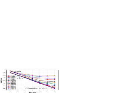
Figure 2: NMSE comparison for LL, PH and DP under different $f_{d}$’s when $N_{t}=192$ and $N_{sch}=20$.

Finally, different $N_{sch}$’s are evaluated in Fig.3. From the figure, it is obvious that the performance difference between PH and DP is subtle when $N_{sch}\geq 20$, and both of them are far better than LL. When $N_{sch}=10$, PH outperforms LL about 2dB at low SNR regime and over 8dB at high SNR regime, meanwhile, it is worse than DP for about 1dB at low SNR regime and 6dB at high SNR regime.

From simulations, we find that PH outperforms LL over a wide range of SNR’s and Doppler’s when the number of observed OFDMA symbols and the number of allocated subchannels are not too small, i.e., $N_{t}\geq 96$ and $N_{sch}\geq 10$.

V Conclusion

In this paper, we propose an ESPRIT-based channel estimation algorithm applicable to uplink OFDMA by exploiting pilot hopping. Through a very simple pilot hopping scheme, the shift-invariance property based on which ESPRIT is capable is acquired. Since this special property is derived from a pair of contiguous OFDMA symbols, no special pilot pattern, e.g., the doublet pilots in [5], is indispensable within one OFDMA symbol. Hence, the proposed algorithm increases the spectrum efficiency and eases the design of the pilot pattern. Estimating the auto-correlation matrix over numbers of OFDMA symbols, the proposed algorithm outperforms the linear local interpolator within a wide range of SNR’s and Doppler’s. Besides, low rank adaptive filter [14] can be integrated to abate the estimation latency.

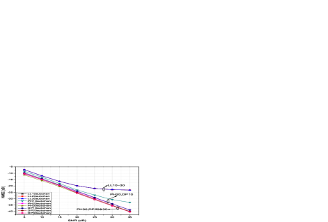
Figure 3: NMSE comparison for LL, PH and DP under different $N_{sch}$’s when $N_{t}=192$ and $f_{d}=200$ Hz.

References

- [1] Draft Standard for Local and Metropolitan Area Networks Part 16 - Air Interface for Fixed Broadband Wireless Access Systems, IEEE Std., March 2007.
- [2] O. Edfors et al., “OFDM Channel Estimation by Singular Value Decompostion,” IEEE Trans. Commun., vol. 46, pp. 931–939, July 1998.
- [3] S. Coleri et al., “Channel Estimation Techniques Based on Pilot Arrangement in OFDM Systems,” IEEE Trans. Broadcast., vol. 48, pp. 223–229, September 2002.
- [4] X. Dong et al., “Linear Interpolation in Pilot Symbol Assisted Channel Estimation for OFDM,” IEEE Trans. Wireless Commun., vol. 6, pp. 1910–1920, May 2007.
- [5] M. Raghavendra et al., “Parametric Channel Estimation for Pseudo-Random Tile-Allocation in Uplink OFDMA,” IEEE Trans. Signal Process., vol. 55, pp. 5370–5381, November 2007.
- [6] B. Yang et al., “Channel Estimation for OFDM Transmission in Multipath Fading Channels Based on Parametric Channel Modeling,” IEEE Trans. Commun., vol. 49, pp. 467–479, March 2001.
- [7] R. Roy and T. Kailath, “ESPRIT - Estimation of Signal Parameters via Rotational Invariance Techniques,” IEEE Trans. Acoust., Speech, Signal Process., vol. 37, pp. 984–995, July 1989.
- [8] M. Wax and T. Kailath, “Detection of Signals by Information Theoretic Criteria,” IEEE Trans. Acoust., Speech, Signal Process., vol. 33, pp. 387–392, April 1985.
- [9] R. Steele, Mobile Radio Communications. New York: IEEE Press, 1992.
- [10] D. Tse and P. Viswanath, Fundamentals of Wireless Communication. New York: Cambridge University Press, 2005.
- [11] M. Raghavendra et al., “Exploiting Hopping Pilots for Parametric Channel Estimation in OFDM Systems,” IEEE Signal Process. Lett., vol. 12, pp. 737–740, November 2005.
- [12] S. Ohno and G. Giannakis, “Capacity Maximizing MMSE-Optimal Pilots for Wireless OFDM Over Frequency-Selective Block Rayleigh-Fading Channels,” IEEE Trans. Inf. Theory, vol. 50, pp. 2138–2145, September 2004.
- [13] “Guidelines for Evaluation of Radio Transmission Technologies for IMT-2000,” Recommendations ITU-R M.1225, 1997.
- [14] P. Strobach, “Low-Rank Adaptive Filters,” IEEE Trans. Signal Process., vol. 44, pp. 2932–2947, December 1996.