Robust Linear Processing for Downlink Multiuser MIMO System With Imperfectly Known Channel

Abstract

In practical systems, due to the time-varying radio channel, the channel state information (CSI) may not be known well at both transmitters and receivers. For most of the current multiuser multiple-input multiple-output (MIMO) schemes, they suffer a significant degression on the performance due to the mismatch between the true and estimated CSI. To alleviate the performance penalty, a robust downlink multiuser MIMO scheme is proposed in this paper by exploiting the channel mean and antenna correlation. These channel statistics are more stable than the imperfect CSI estimation in the time-varying radio channel, and they are used, in the proposed scheme, to minimize the total mean squared error under the sum power constraint. Simulation results demonstrate that the proposed scheme effectively mitigates the performance loss due to the CSI mismatch.

I Introduction

The multiple-input multiple-output (MIMO) system, employing multiple transmit and receive antennas, has been recognized as an effective way to improve the spectral efficiency of the radio channel [1] [2]. More recently, multiuser schemes have been investigated for MIMO systems to further improve the multiuser sum capacity.

Early studies have assumed a perfectly knowledge of the channel state information (CSI) available at the transmitter. [3] extended the single-user scheme [4] to the multiuser system. However, without exploring the multiuser channel information, it simply treated the multiuser interference as the white noise. The scheme in [5], on the contrary, utilized the multiuser information effectively to minimize the total mean squared error (TMMSE) and, naturally, possessed a better performance.

The CSI can be obtained at the transmitter either by using a feedback channel from the receiver to the transmitter in frequency division duplex (FDD) systems, or by invoking the channel reciprocity in time division duplex (TDD) systems. However, using feedback in FDD systems, the limited resources for the feedback, associated with the propagation delay and schedule lag, heavily degrade the accuracy of the CSI at the transmitter. As to the channel reciprocity in TDD systems, the accuracy of the CSI is corrupted by antenna calibration errors and turn-around time delay. In respect that the performance would degrade significantly under the imperfect CSI, it is necessary to design a multiuser scheme which is stable to the imperfect CSI.

In robust design methodologies, Maxmin (worst-case) and Bayesian (stochastic) are two well known ones [7]. The former optimizes the performance under the worst case of random channels, thus, it is so conservative that its average performance is even worse than non-robust schemes [8]. The latter maximizes the ensemble average performance over a pre-described stochastic distribution of the CSI. When the stochastic distribution matches well with the true CSI, the latter outperforms the former.

The scheme in [7] was a Bayesian design for downlink multiuser MIMO systems with the imperfectly known CSI. It introduced a channel error matrix to the cost function of [3], then found the solution which minimized the average cost. However, similar with [3], the multiuser interference was also treated as the white noise. Therefore, it is expected that the performance can be improved by exploring the multiuser information.

In this paper, a robust scheme for downlink multiuser MIMO systems is proposed based on the TMMSE criterion. A more general channel model involving the channel mean and antenna correlation is considered. The scheme is a Bayesian design which minimizes the average cost function under the sum power constraint.

The rest of this paper is organized as follows. The channel model and problem formulation are described in Section II. The Section III presents the design of the robust multiuser scheme for the correlated imperfect known channel under the sum power constraint. Simulation results and analysis are given in Section IV. Finally, the Section V concludes the paper.

Notation: Boldface upper-case letters denote matrices, and boldface lower-case letters denote column vectors. $tr(\cdot)$, $(\cdot)^{*}$, $(\cdot)^{H}$, $||\cdot||_{2}$ and $||\cdot||_{F}$ denote trace, conjugate, conjugate transposition, Euclidian norm and Frobenius norm, respectively. $E(\cdot)$ represents the expectation of a stochastic process. $[{\bf{\cdot}}]_{i,j}$, $[{\bf{\cdot}}]_{{\bf{:}},j}$ denote the $(i$,$j)$-th element and $j$-th column of a matrix, respectively.

II Problem statement

II-A Channel Model

Consider a base station (BS) with $M$ antennas and $K$ mobile stations (MS’s) each having $N_{i}(i=1\dots K)$ antennas. Represented by a matrix ${\bf{H}}_{i}\in\mathcal{C}^{N_{i}\times M}$, the downlink MIMO channel to MS_i is assumed to be frequency-flat and quasi-static block fading. Suppose a non-zero-mean channel with both transmit and receive antenna correlations, ${\bf{H}}_{i}$ is written as follows [9][11]

$${\bf{H}}_{i}=\sqrt{\frac{{W_{i}}}{{W_{i}+1}}}{\bf{\tilde{H}}}_{0,i}+\sqrt{\frac{1}{{W_{i}+1}}}{\bf{R}}_{0,r,i}^{\frac{1}{2}}{\bf{\Delta}}_{i}{\bf{R}}_{t}^{\frac{1}{2}}$$ (1)

where $W_{i}$ is the ratio of the power in the mean component to the average power in the variant component of ${\bf{H}}_{i}$; ${\bf{\Delta}}_{i}\in\mathcal{C}^{N_{i}\times N_{i}}$ is random, we assume that its entries form an independent identical distribution (i.i.d.) complex Gaussian collection with zero-mean and identity covariance, i.e., ${\bf{\Delta}}_{i}\sim\mathcal{CN}(0,1)$; ${\bf{\tilde{H}}}_{0,i}\in\mathcal{C}^{N_{i}\times M}$ is the normalized channel mean, and ${\bf{R}}_{0,r,i}\in\mathcal{C}^{N_{i}\times N_{i}}$ and ${\bf{R}}_{t}\in\mathcal{C}^{M\times M}$ are the normalized correlation matrices of the receiver of MS_i and the transmitter of BS, respectively. (1) is rewritten into the following for simplicity [11]

$${\bf{H}}_{i}={\bf{\tilde{H}}}_{i}+{\bf{R}}_{r,i}^{\frac{1}{2}}{\bf{\Delta}}_{i}{\bf{R}}_{t}^{\frac{1}{2}}$$ (2)

where ${\bf{\tilde{H}}}_{i}=\sqrt{W_{i}/(W_{i}+1)}{\bf{\tilde{H}}}_{0,i}$ is the channel mean, and ${\bf{R}}_{r,i}=1/(W_{i}+1){\bf{R}}_{0,r,i}$ is the equivalent correlation matrix of the receiver of MS_i.

The channel mean and correlation are more stable than the instantaneous channel information, and they are usually acquired by time-averaging on channel measurements. In the Rayleigh channel, for example, the non-zero channel mean ${\bf{\tilde{H}}}_{i}$ is obtained by averaging channel measurements over a window of tens of the channel coherence time [10]. Furthermore, the channel model (2) can also denote the correlated Rician MIMO channel, in which case the channel mean represents the line-of-sight (LOS) component of the MIMO channel.

In this paper, we assume that transmitters and receivers only know channel means and antenna correlations.

II-B Problem Formulation

We assume that there are $L_{i}(i=1\dots K)$ substreams between BS and MS${}_{i}(i=1\dots K)$, that is to say, BS transmits $L_{i}$ symbols to MS_i simultaneously. Then the signal received at MS_i is

$${\bf{y}}_{i}={\bf{A}}_{i}^{H}{\bf{H}}_{i}\sum\limits_{k=1}^{K}{{\bf{B}}_{k}{\bf{x}}_{k}}+{\bf{A}}_{i}^{H}{\bf{n}}_{i}$$ (3)

where ${\bf{y}}_{i}\in\mathcal{C}^{N_{i}\times 1}$ is the received signal vector, and ${\bf{x}}_{i}\in\mathcal{C}^{L_{i}\times 1}$ is the transmitted signal vector from BS to MS_i with zero-mean and normalized covariance matrix $\mathbf{I}$. We assume the transmitted signal vectors of different users are uncorrelated, i.e., $E\left({{\bf{x}}_{i}{\bf{x}}_{j}^{H}}\right)=\delta_{ij}\bf{I}$, where ${\delta_{ij}}$ is the Kronecker function, ${\delta_{ij}=1}$, when ${i=j}$ and ${\delta_{ij}=0}$, when ${i\neq j}$. We also assume the noise vector is independent of any signal vector. A linear post-filter ${\bf{A}}_{i}\in\mathcal{C}^{N_{i}\times L_{i}}(i=1\dots K)$ is used at MS_i to recover an estimation of the transmitted signal vector ${\bf{x}}_{i}$. ${\bf{H}}_{i}$ defined in (1) [or (2)] denotes the MIMO channel from BS to MS_i. ${\bf{B}}_{i}\in\mathcal{C}^{M\times L_{i}}(i=1\dots K)$ is used at BS to weight the transmitted signal vector ${\bf{x}}_{i}$. After passing through ${\bf{B}}_{i}$, ${\bf{x}}_{i}$ becomes into an $M\times 1$ signal vector which is transmitted by $M$ transmit antennas of BS. ${\bf{n}}_{i}\in\mathcal{C}^{N_{i}\times 1}$ is the noise vector with the correlation matrix ${\bf{R}}_{n_{i}}=\sigma_{n}^{2}{\bf{I}}_{{\bf{N}}_{i}}$, where ${\bf{I}}_{{\bf{N}}_{i}}$ denotes the ${{\bf{N}}_{i}}\times{{\bf{N}}_{i}}$ identity matrix. In this paper, we assume $L_{1}=\dots=L_{K}=L$.

$\mathbf{A}_{i}$ and $\mathbf{B}_{i}$ $(k=1\dots K)$ are jointly designed to minimize the total MSE under the sum power constraint. Hence, we get

$$\begin{array}[]{cl}{\min}&{TMSE=E\left(\sum\limits_{k=1}^{K}{||{\bf{x}}_{k}-{\bf{y}}_{k}||^{2}}\right)}\\ {s.t.}&{tr\left(\sum\limits_{k=1}^{K}{{\bf{B}}_{k}{\bf{B}}_{k}^{H}}\right)\leq P}\\ \end{array}$$ (4)

where $P$ is the total transmit power of BS.

III Robust TMMSE Scheme

According to (3), the $j$-th user’s MSE is

$$\begin{array}[]{lll}MSE_{j}&=&E\left({||{\bf{x}}_{j}-{\bf{y}}_{j}||^{2}}\right)\\ &=&E(tr({\bf{A}}_{j}^{H}{\bf{H}}_{j}(\sum\limits_{i=1}^{K}{{\bf{B}}_{i}{\bf{B}}_{i}^{H}}){\bf{H}}_{j}^{H}{\bf{A}}_{j}+\sigma_{n}^{2}{\bf{A}}_{j}^{H}{\bf{A}}_{j}\\ &&-{\bf{B}}_{j}^{H}{\bf{H}}_{j}^{H}{\bf{A}}_{j}-{\bf{A}}_{j}^{H}{\bf{H}}_{j}{\bf{B}}_{j}+{\bf{I}}))\\ \end{array}$$ (5)

Substitute (2) into (5) and note $E\left({\bf{H}}_{i}\right)={\bf{\tilde{H}}}_{i}$, hence $E\left({\bf{R}}_{r,i}^{\frac{1}{2}}{\bf{\Delta}}_{i}{\bf{R}}_{t}^{\frac{1}{2}}\right)={\bf{0}}$, we obtain

$$\begin{array}[]{lll}MSE_{j}&=&tr({\bf{A}}_{j}^{H}{\bf{\tilde{H}}}_{j}(\sum\limits_{i=1}^{K}{{\bf{B}}_{i}{\bf{B}}_{i}^{H}}){\bf{\tilde{H}}}_{j}^{H}{\bf{A}}_{j}+\sigma_{n}^{2}{\bf{A}}_{j}^{H}{\bf{A}}_{j}\\ &{}&-{\bf{B}}_{j}^{H}{\bf{\tilde{H}}}_{j}^{H}{\bf{A}}_{j}-{\bf{A}}_{j}^{H}{\bf{\tilde{H}}}_{j}{\bf{B}}_{j}+{\bf{I}})+E(tr({\bf{A}}_{j}^{H}\\ &{}&{\bf{R}}_{r,j}^{\frac{1}{2}}{\bf{\Delta}}_{j}{\bf{R}}_{t}^{\frac{1}{2}}(\sum\limits_{i=1}^{K}{{\bf{B}}_{i}{\bf{B}}_{i}^{H}}){\bf{R}}_{t}^{\frac{1}{2}H}{\bf{\Delta}}_{j}^{H}{\bf{R}}_{r,j}^{\frac{1}{2}H}{\bf{A}}_{j}))\\ \end{array}$$ (6)

Observe the last part in (6)

$$\begin{array}[]{ll}E(tr({\bf{A}}_{j}^{H}{\bf{R}}_{r,j}^{\frac{1}{2}}{\bf{\Delta}}_{j}{\bf{R}}_{t}^{\frac{1}{2}}(\sum\limits_{i=1}^{K}{{\bf{B}}_{i}{\bf{B}}_{i}^{H}}){\bf{R}}_{t}^{\frac{1}{2}H}{\bf{\Delta}}_{j}^{H}{\bf{R}}_{r,j}^{\frac{1}{2}H}{\bf{A}}_{j}))\\ {\;\;\;}={\;}tr({\bf{R}}_{t}^{\frac{1}{2}}(\sum\limits_{i=1}^{K}{{\bf{B}}_{i}{\bf{B}}_{i}^{H}}){\bf{R}}_{t}^{\frac{1}{2}H}E({\bf{\Delta}}_{j}^{H}{\bf{R}}_{r,j}^{\frac{1}{2}H}{\bf{A}}_{j}{\bf{A}}_{j}^{H}{\bf{R}}_{r,j}^{\frac{1}{2}}{\bf{\Delta}}_{j}))\\ \end{array}$$ (7)

Moreover, as ${\bf{\Delta}}_{i}\sim\mathcal{CN}(0,1)$ with i.i.d. entries, $E(\left[{\bf{\Delta}}_{j}\right]_{:,n}(\left[{\bf{\Delta}}_{j}\right]_{:,m})^{H})=\delta_{n,m}\bf{I}$. Therefore, the $(m$,$n)$-th entry of the expectation in the right side of (7) is

$$\begin{array}[]{llll}E(\left[{\bf{\Delta}}_{j}^{H}{\bf{R}}_{r,j}^{\frac{1}{2}H}{\bf{A}}_{j}{\bf{A}}_{j}^{H}{\bf{R}}_{r,j}^{\frac{1}{2}}{\bf{\Delta}}_{j}\right]_{m,n})&{}&\\ {\;\;\;\;\;\;\;\;\;\;\;\;\;}\begin{array}[]{llll}=&E((\left[{\bf{\Delta}}_{j}\right]_{:,m})^{H}{\bf{R}}_{r,j}^{\frac{1}{2}H}{\bf{A}}_{j}{\bf{A}}_{j}^{H}{\bf{R}}_{r,j}^{\frac{1}{2}}\left[{\bf{\Delta}}_{j}\right]_{:,n})\\ =&tr({\bf{R}}_{r,j}^{\frac{1}{2}H}{\bf{A}}_{j}{\bf{A}}_{j}^{H}{\bf{R}}_{r,j}^{\frac{1}{2}}E(\left[{\bf{\Delta}}_{j}\right]_{:,n}(\left[{\bf{\Delta}}_{j}\right]_{:,m})^{H}))\\ =&\delta_{n,m}tr({\bf{R}}_{r,j}^{\frac{1}{2}H}{\bf{A}}_{j}{\bf{A}}_{j}^{H}{\bf{R}}_{r,j}^{\frac{1}{2}})\\ =&\delta_{n,m}tr({\bf{A}}_{j}^{H}{\bf{R}}_{r,j}{{\bf{A}}_{j}})\\ \end{array}\end{array}$$ (8)

Thus, the expectation in the right side of (7) is

$$E({{\bf{\Delta}}_{j}^{H}{\bf{R}}_{r,j}^{\frac{1}{2}H}{\bf{A}}_{j}{\bf{A}}_{j}^{H}{\bf{R}}_{r,j}^{\frac{1}{2}}{\bf{\Delta}}_{j}})=tr({\bf{A}}_{j}^{H}{\bf{R}}_{r,j}{{\bf{A}}_{j}}){\bf{I}}$$ (9)

Substitute (9) into (7), we obtain

$$\begin{array}[]{lll}E(tr({\bf{A}}_{j}^{H}{\bf{R}}_{r,j}^{\frac{1}{2}}{\bf{\Delta}}_{j}{\bf{R}}_{t}^{\frac{1}{2}}(\sum\limits_{i=1}^{K}{{\bf{B}}_{i}{\bf{B}}_{i}^{H}}){\bf{R}}_{t}^{\frac{1}{2}H}{\bf{\Delta}}_{j}^{H}{\bf{R}}_{r,j}^{\frac{1}{2}H}{\bf{A}}_{j}))\\ {\;\;\;}={\;}tr({\bf{R}}_{t}^{\frac{1}{2}}(\sum\limits_{i=1}^{K}{{\bf{B}}_{i}{\bf{B}}_{i}^{H}}){\bf{R}}_{t}^{\frac{1}{2}H}tr({\bf{A}}_{j}^{H}{\bf{R}}_{r,j}{{\bf{A}}_{j}}){\bf{I}})\\ {\;\;\;}={\;}tr({\bf{A}}_{j}^{H}{\bf{R}}_{r,j}{{\bf{A}}_{j}})tr((\sum\limits_{i=1}^{K}{{\bf{B}}_{i}{\bf{B}}_{i}^{H}}){\bf{R}}_{t})\\ \end{array}$$ (10)

Substitute (10) into (6)

$$\begin{array}[]{lll}MSE_{j}&=&tr({\bf{A}}_{j}^{H}{\bf{\tilde{H}}}_{j}(\sum\limits_{i=1}^{K}{{\bf{B}}_{i}{\bf{B}}_{i}^{H}}){\bf{\tilde{H}}}_{j}^{H}{\bf{A}}_{j}+\sigma_{n}^{2}{\bf{A}}_{j}^{H}{\bf{A}}_{j}\\ &{}&-{\bf{B}}_{j}^{H}{\bf{\tilde{H}}}_{j}^{H}{\bf{A}}_{j}-{\bf{A}}_{j}^{H}{\bf{\tilde{H}}}_{j}{\bf{B}}_{j}+{\bf{I}})\\ &{}&+tr({\bf{A}}_{j}^{H}{\bf{R}}_{r,j}{{\bf{A}}_{j}})tr((\sum\limits_{i=1}^{K}{{\bf{B}}_{i}{\bf{B}}_{i}^{H}}){\bf{R}}_{t})\\ \end{array}$$ (11)

The Lagrangian of (4) is

$$\begin{array}[]{lll}L({\bf{A}}_{1},\dots,{\bf{A}}_{K},{\bf{B}}_{1},\dots,{\bf{B}}_{K})&{}&\\ {\;\;\;\;\;\;\;\;\;\;\;\;\;}=\sum\limits_{k=1}^{K}MSE_{k}+\lambda({tr(\sum\limits_{k=1}^{K}{{\bf{B}}_{k}{\bf{B}}_{k}^{H}})-P})\end{array}$$ (12)

where $\lambda$ is the Lagrangian multiplier associated with the total power constraint. So the Karush-Kuhn-Tucker (KKT) conditions [10] of (4) are

$$\frac{{\partial L({\bf{A}}_{1},...,{\bf{A}}_{K},{\bf{B}}_{1},...,{\bf{B}}_{K})}}{{\partial{\bf{A}}_{i}^{*}}} = \bf{0}$$ (13)

$$\frac{{\partial L({\bf{A}}_{1},...,{\bf{A}}_{K},{\bf{B}}_{1},...,{\bf{B}}_{K})}}{{\partial{\bf{B}}_{i}^{*}}} = \bf{0}$$ (14)

$$\lambda\left({tr(\sum\limits_{i=1}^{K}{{\bf{B}}_{i}{\bf{B}}_{i}^{H}})-P}\right) = 0$$ (15)

$$\lambda \geq 0$$ (16)

Among them, (13)(14) come from the fact that the gradients of the Lagrangian (12) definitely vanish at the optimal point, and (15) is known as the complementary slackness. According to (11)$\sim$(14), we obtain

$$\begin{array}[]{lll}{\bf{A}}_{i}=&({\bf{\tilde{H}}}_{i}(\sum\limits_{k=1}^{K}{{\bf{B}}_{k}{\bf{B}}_{k}^{H}}){\bf{\tilde{H}}}_{i}^{H}+tr((\sum\limits_{k=1}^{K}{{\bf{B}}_{k}{\bf{B}}_{k}^{H}}){\bf{R}}_{t}){\bf{R}}_{r,i}\\ &+\sigma_{n}^{2}{\bf{I}})^{-1}{\bf{\tilde{H}}}_{i}{\bf{B}}_{i}\end{array}$$ (17)

$$\begin{array}[]{lll}{\bf{B}}_{i}=&(\sum\limits_{k=1}^{K}{{\bf{\tilde{H}}}_{k}^{H}{\bf{A}}_{k}{\bf{A}}_{k}^{H}{\bf{\tilde{H}}}_{k}}+tr(\sum\limits_{k=1}^{K}{{\bf{A}}_{k}{\bf{A}}_{k}^{H}{\bf{R}}_{r,k}}){\bf{R}}_{t}\\ &+\lambda{\bf{I}})^{-1}{\bf{\tilde{H}}}_{i}^{H}{\bf{A}}_{i}\end{array}$$ (18)

Substitute (18) into (15) , we can find $\lambda$ is the root of the equation

$$\lambda(tr\left({{\bf{X}}({\bf{X}}+{\bf{Y}}+\lambda{\bf{I}}}\right)^{-2})-P)=0$$ (19)

where

$${\bf{X}}=\sum\limits_{k=1}^{K}{{\bf{\tilde{H}}}_{k}^{H}{\bf{A}}_{k}{\bf{A}}_{k}^{H}{\bf{\tilde{H}}}_{k}}$$ (20)

$${\bf{Y}}=tr(\sum\limits_{k=1}^{K}{{\bf{A}}_{k}{\bf{A}}_{k}^{H}{\bf{R}}_{r,k}}){\bf{R}}_{t}$$ (21)

As ${\bf{R}}_{t}$ is the normalized correlation matrix of the transmitter, it is Hermitian, hence both $\bf{X}$ and $\bf{Y}$ are Hermitian, and so is $\bf{X}+\bf{Y}$. Perform the eigenvalue decomposition

$${\bf{X}}+{\bf{Y}}={\bf{UDU}}^{H}$$ (22)

where $\bf{U}$ is unitary and $\bf{D}$ is diagonal. If $\lambda\neq 0$, (19) can be rewritten to

$$\sum\limits_{n=1}^{M}{\frac{{\left[{{\bf{U}}^{H}{\bf{XU}}}\right]_{n,n}}}{{(d_{n}+\lambda)^{2}}}}-P=0$$ (23)

where $d_{n}$ is the $n$-th diagonal element of $\mathbf{D}$. Using a binary search, the root of (23) can be found quickly. Since the left-hand side of (23) is monotonous in $\lambda$ when $\lambda\geq 0$, the upper and lower bounds on $\lambda$ can be acquired by replacing $d_{n}$ with $d_{min}$ and $d_{max}$, respectively. Thus,

$$\lambda_{upper}=\left({\sqrt{\frac{{tr(\bf{X})}}{P}}-d_{\min}}\right)^{+}$$ (24)

$$\lambda_{lower}=\left({\sqrt{\frac{{tr(\bf{X})}}{P}}-d_{\max}}\right)^{+}$$ (25)

where $(\cdot)^{+}$ means that the expression takes the value inside the parentheses if the value is positive, otherwise it takes zero. A numerical binary search, then, can be carried out between these two bounds to find the root of (23) up to a desired precision. Once there is no root between the bounds, which implies that the inequality constraint (16) is inactive, $\lambda=0$ is the only available solution to (18). From (17) (18), it can be found that the optimal transmit matrices ${\bf{B}}_{k}(k=1\dots K)$ are functions of the receive matrices ${\bf{A}}_{k}(k=1\dots K)$, and vice versa. Therefore an iterative algorithm to calculate ${\bf{A}}_{k}$ and ${\bf{B}}_{k}(k=1\dots K)$ is proposed as follows.

  Initialize ${\bf{B}}_{k}^{(0)}$ and ${\bf{A}}_{k}^{(0)}$ $(k=1\dots K)$ randomly. $n=0$

  1) Calculate $\lambda$ from ${\bf{A}}_{k}^{(n)}$ $(k=1\dots K)$ by solving (19).

  2) Calculate ${\bf{B}}_{k}^{(n+1)}(k=1\dots K)$ from ${\bf{A}}_{k}^{(n)}$ $(k=1\dots K)$ and $\lambda$ using (18).

  3) Calculate ${\bf{A}}_{k}^{(n+1)}(k=1\dots K)$ from ${\bf{B}}_{k}^{(n+1)}$ $(k=1\dots K)$ using (17).

  4) Repeat 1), 2) and 3) until $\sum\limits_{k=1}^{K}({||{\bf{A}}_{k}^{(n+1)}-{\bf{A}}_{k}^{(n)}||_{F}^{2}+||{\bf{B}}_{k}^{(n+1)}-{\bf{B}}_{k}^{(n)}||_{F}^{2}})<\varepsilon$. In our simulation, we set $\varepsilon=0.0001$.

IV Simulation results

In this section, numerical simulations have been carried out to evaluate the performance of the proposed scheme. We assume that the BS equipped with four antennas ($M=4$) is communicating with two MS’s ($K=2$) each with $N$ receive antennas ($N_{1}=N_{2}=N$). Also we assume that the number of substreams of each MS is equal to $2$ $(L_{1}=L_{2}=2)$, moreover, both the two MS’s have the same $W_{i}$ $(W_{1}=W_{2}=W)$. QPSK is employed in the simulations and no channel coding is considered. Let the transmit antenna correlation matrix ${\bf{R}}_{t}$ be $\left[{{\bf{R}}_{t}}\right]_{i,j}=0.9^{|i-j|}$ and the receive antennas be uncorrelated, i.e., ${\bf{R}}_{r,i}={\bf{I}}_{N}$.

Firstly, we compare the bit error rate (BER) of the proposed robust TMMSE scheme with that of the traditional TMMSE scheme. Defining the signal-to-noise ratio (SNR) as the ratio of total transmitted power to the noise power of each antenna ($SNR=P/\sigma_{n}^{2}$), Fig. 1 is the average BER curves versus the SNR When $N=2$. In order to highlight its impact on the BER performance, different values of $W$ are used in the evaluations. When $W$ is small, the channel mean poorly reflects the instantaneous channel state, thus the receiver can not completely eliminate the interference among the transmitted signals, which further induces an irreducible error floor at high SNR region. However, the proposed robust scheme overcomes the traditional one with a noticeable gain. As the $W$ increases, the transmitter obtains more precise CSI, therefore the residual interference is mitigated greatly and the error floor vanishes. In addition, the gain between the proposed robust scheme and the traditional one turns small when the uncertainty of the channel state is decreasing.

In Fig. 2, we compare the BER performance when the number of receive antennas is increasing. The additional receive antennas provide more spatial diversity gain. In this figure, $W$ is fixed to be $50$ and $N$ changes from $2$ to $4$. Although both the two schemes explore the additional receive diversity gain, the proposed robust scheme obviously has a better performance for all $N$’s due to its insensitivity to the imperfect CSI.

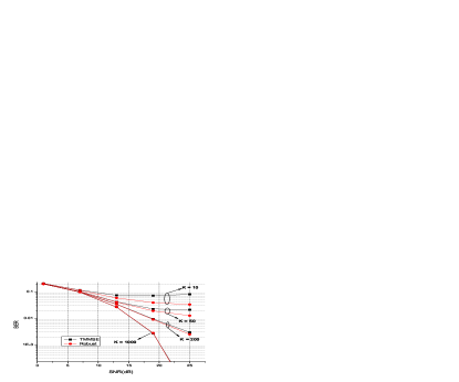
Figure 1: Comparison of the BER performance of the robust scheme and the TMMSE, when $N=2$ and $W=10,50,200,1000$.

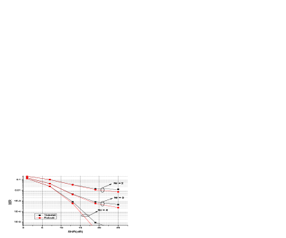
Figure 2: Comparison of the BER performance of the robust scheme and the TMMSE, when $N=2,3,4$ and $W=50$.

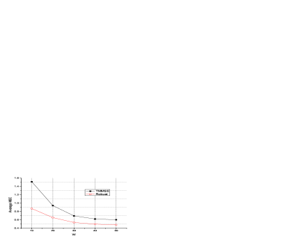
Figure 3: Comparison of the average MSE of the robust scheme and the TMMSE, when $N=2$ and $SNR=20$dB.

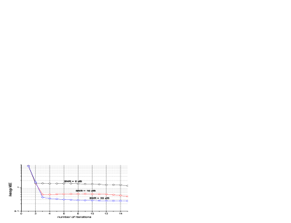
Figure 4: Convergence of the robust scheme, when $N=2$ and $W=100$.

Fig. 3 shows the average MSE as a function of $W$, when SNR = $20$dB and $N=2$. The average MSE of the proposed robust scheme is less than that of the traditional TMMSE scheme over all $W$’s. Moreover, compared to the traditional TMMSE, the descending slope of the proposed robust scheme is flat, which further indicates that its performance is insensitive to the channel uncertainty. Especially when $W$ becomes larger, more reliable CSI is available, therefore closer the two curves get.

Fig. 4 illustrates the convergence property of the proposed robust scheme, when $N=2$, $W=100$. The curves of the average MSE versus the number of iterations needed in different SNR’s are plotted. The higher the SNR is, the more iterations the proposed scheme runs for to converge. Fortunately, for the most SNR’s, four iterations are big enough to guarantee the convergence.

V Conclusion

In this paper, we investigate a robust linear processing scheme for the downlink multiuser MIMO system under the consideration of imperfect CSI. As the traditional downlink multiuser MIMO systems depend on the instantaneous CSI too much, they suffer poor performance once the CSI is not accurate enough. In order to deliver a better performance under the imperfect CSI, an iterative Bayesian algorithm which explores channel statistics to offer a much more stable description to the channel state is developed by minimize the total MSE under the sum power constraint. Numerical simulations exhibit the proposed robust scheme experiences an obvious performance gain over the traditional schemes. In addition, the proposed iterative algorithm has a good convergence property – after no more than four times of iterations, the algorithm achieves convergence.

References

• [1] I. Telatar, ”Capacity of multi-antenna Gaussian channels”, Eur. Trans. Telecommun., vol. 10, no. 6, pp. 585-595, Nov./Dec. 1999.
• [2] Q. Caire and S. Shamai, ”On the achievable throughput of a multiantenna gaussian broadcast channel”, IEEE Trans. Inf. Theory, vol. 49, no. 7, pp. 1691-1706, July 2003.
• [3] A.J.Tenenbaum and R.S.Adve, ”Joint multiuser transmit-receive optimization using linear processing”, IEEE Intl. Conf. on Commun., vol.1, pp.588-592, June 2004.
• [4] D.P.Palomar, J.M.Cioffi, and M.A.Lagunas, ”Joint Tx-Rx beamforming design for multicarrier MIMO channels: a unified framework for convex optimization”, IEEE Trans. Signal Processing, vol.51, pp.2381-2401, Sept. 2003.
• [5] J.F. Zhang and M.G. Xu, ”Minimum system-wide mean-squared error for downlink spatial multiplexing in multiuser MIMO channels”, in proc. IEEE golbalcom’05, vol. 5, pp. 4, DEC. 2005.
• [6] M. Vu and A. Paulraj, ”MIMO Wireless Precoding”, IEEE Signal Processing Magazine, accepted in 2006.
• [7] H. Li and C.Q. Xu, ”Robust Optimization of Linear Precoders/Decoders for Multiuser MIMO Downlink with Imperfect CSI at Base Station”, in proc. IEEE WCNC’07, pp. 1129-1133, Mar. 2007.
• [8] H.T. Sun and Z. Ding, ”Robust precoder design for MIMO packet retransmissions over imperfectly known flat-fading channels”, in proc. IEEE ICC, vol.7, pp. 3287-3292, June 2006.
• [9] A. Hjorungnes, D. Gesbert and J. Akhtar, ”Precoding of Space-Time Block Coded Signals for Joint Transmit-Receive Correlated MIMO Channels”, IEEE Trans. Wireless Commun., vol.5, pp.492-497, Mar. 2006.
• [10] S. Boyd and L. Vandenberghe, Convex Optimization, Cambridge: U.K. Cambridge University Press, 2004.
• [11] M. Vu and A. Paulraj, ”Optimal Linear Precoders for MIMO Wireless Correlated Channels With Nonzero Mean in Space-Time Coded Systems”, IEEE Trans. Signal Processing, vol. 54, no. 6, pp. 2318-2332, June 2006.