Variable Evolved Stars and YSOs Discovered in the Large Magellanic Cloud using the SAGE Survey

Abstract

We present initial results and source lists of variable sources in the Large Magellanic Cloud (LMC) for which we detect thermal infrared variability from the SAGE (Surveying the Agents of a Galaxy’s Evolution) survey, which had 2 epochs of photometry separated by three months. The SAGE survey mapped a $7\arcdeg\times 7\arcdeg$ region of the LMC using the IRAC and the MIPS instruments on board Spitzer. Variable sources are identified using a combination of the IRAC 3.6, 4.5, 5.8, 8.0 µm bands and the MIPS 24 µm bands. An error-weighted flux difference between the two epochs is used to assess the variability. Of the $\sim 3$ million sources detected at both epochs we find $\sim 2,000$ variable sources for which we provide electronic catalogs. Most of the variable sources can be classified as asymptotic giant branch (AGB) stars. A large fraction ($>66\%$) of the extreme AGB stars are variable and only smaller fractions of carbon-rich (6.1%) and oxygen-rich (2.0%) stars are detected as variable. We also detect a population of variable young stellar object candidates.

1 Introduction

The Spitzer survey, Surveying the Agents of a Galaxy’s Evolution (SAGE) of the Large Magellanic Cloud (LMC) provides an unprecedented opportunity to detect thermal infrared variability of the infrared stellar population of the LMC. Optical variability studies of the LMC by the MACHO (Alcock et al., 1996) and OGLE (Paczynski et al., 1994) monitoring projects have revealed the period and luminosity relations for a wide variety of variable stars in the LMC, e.g. the long period variables (Fraser et al., 2005). The three month time span between the two epochs of observations for the SAGE survey can detect and constrain the variability of long period variables in the evolved star population and young stellar object candidates. Thermal infrared variability of such objects has been studied in the Galaxy with IRAS and ISO, and Spitzer’s improved sensitivity enables such studies in nearby galaxies. The  10 month IRAS mission surveyed most portions of the sky at least twice a year, separated by months and thus also constrained variability of the brighter infrared sources in a similar way that the SAGE data samples the LMC’s stellar populations.

Most of the sources detected as variables in the thermal infrared by IRAS or ISO are evolved stars in our Galaxy. For example, Harmon & Gilmore (1988) used the IRAS VAR index to determine the nature of the IRAS stellar population that delineates the Galactic Bulge. In a statistical way, they simulated the periods that the IRAS data were sensitive to and found the data were most sensitive to long period variables, P$>$ 400 days up to 1,400 days. Essentially, large amplitude and long period variations are easier to detect and are also associated with larger mass-loss rates. They used this period to estimate the age and mass range for this evolved stellar population in the bulge. Later work by van der Veen & Habing (1990) also used the IRAS VAR to select and study OH/IR stars for ground based measurements of infrared light curves and find that these IRAS variables fit well into the period-luminosity relations found for Mira variables in Baade windows, confirming that OH/IR stars are more evolved forms of Miras. ISOGal-DENIS studies of the Galactic bulge included one field with multiple ISOCam images separated by 17 – 23 months (Omont et al., 1999). This study revealed a population of red giants with weak mass loss for which the brightest, and most dusty red giants have variation at 7 and 15 µm. These sources are “intermediate aymptotic giant branch (AGB) stars” i.e. between early AGB and thermally pulsing AGBs, and have low mass loss rates, $10^{-10}$ to $10^{-11}$ M_⊙ yr^-1.

In the LMC, the evolved stars are too faint for IRAS and ISO measurements to reliably detect variability. However, IRAS- and ISO- detected evolved stars have been followed up by ground based near-IR variability monitoring programs. Whitelock et al. (2003) monitored the IRAS-selected sample of AGB stars studied by ISO and find that larger amplitude variations in K are associated with redder stars. The IRAS and ISO photometry are sensitive measures of dusty mass-loss of the AGB stars. Luminosity is correlated with period and longer periods have higher amplitude variations. Thus, the thermal infrared variability of the evolved stars can cause a systematic scatter in the mass-loss rate determinations of these evolved stars in the LMC and in mass-loss rate vs. luminosity relations (Groenewegen et al., 2007).

In contrast to the evolved star populations, there have been few thermal infrared variability measurements of young stellar objects (YSOs). IRAS measurements of variability of YSOs were at best difficult due to the low spatial resolution of IRAS and the confusion with diffuse ISM emission. Nevertheless, for isolated YSOs there was a detection of variability at 12 and 25 µm for the Herbig Ae/Be stars AB Aur and WW Vul (Prusti & Mitskevich, 1994). Intermediate mass pre-main sequence stars like UX Ori stars show large photometric and polarimetric variations (Natta et al., 1997). A concurrent ISO and ground based optical monitoring program of UX Ori type stars, SV Cep, was performed by Juhász et al. (2007). Juhász et al. (2007) found that the mid-infrared flux variations were anti-correlated with the optical variations, but that the far-infrared flux variations were positively correlated with the optical variability. They used the infrared variability to help discriminate between disk or disk+envelope models and find that disk models are in better agreement with the data. Ábrahám et al. (2004) used ISO to monitor the long term IR evolution of seven FU Orionis stars. They detected variation in four sources, which provides tentative support for the Hartmann & Kenyon (1985) models for accretion outbursts in FU Ori objects as opposed to precessing jets (Herbig et al., 2003). Interestingly, more luminous stars which appear to have similar characteristics as the FU Orionis stars have no detected outbursts. Chromospheric hot-spots or accretion disk variability can cause optical variability in pre-main sequence stars like T Tauri stars, but these types of objects have very low infrared excesses and are unlikely to be in our list. Our list would include earlier stages of YSOs that have more substantial infrared excesses. Thus, while difficult to detect, thermal infrared variability of YSOs will provide key insights into the structure of YSOs and the physical mechanisms of the star formation process.

In this paper, we present initial results and source lists of SAGE point sources for which we have detected thermal infrared variability between the epoch 1 and 2 photometry measurements. In §2, we outline the method of our approach to detect this variability. In §3, we discuss the results of the variable source selection and their identification of evolved stars and YSOs. In §4, we discuss implications of the results and summarize the main conclusions in §5.

2 Method: Source Selection

SAGE is a Legacy project on the Spitzer Space telescope (Werner et al., 2004), which mapped a $7\arcdeg\times 7\arcdeg$ region of the Large Magellanic Cloud (LMC) using the IRAC camera in the [3.6], [4.5], [5.8], and [8.0] micron bands (Fazio et al., 2004) and the MIPS camera in the [24], [70], and [160] micron filters (Rieke et al., 2004). The scientific goals of the survey focus on the life cycle of baryonic matter, as traced by dust emission, from its start in the interstellar medium (ISM), to the formation of new stars, to the death of these stars and the return of matter to the ISM. The survey was done over two epochs with a total observing time of 291 hrs with IRAC and 217 hrs with MIPS. The details of the survey are described in Meixner et al. (2006). The SAGE photometric data have been separately extracted from the two epochs, that are separated by 3 months. The IRAC epoch 1 data were taken on July 15 – 26, 2005, epoch 2 on Oct 26 – Nov 2, 2005 and the MIPS epoch 1 data were taken on July 27– Aug 3, 2005 and epoch 2 on Nov 2 – 9, 2005. The SAGE Epoch 1 point source catalogs containing over 4 million sources of IRAC (SAGEcatalogIRACepoch1) and over 40,000 sources of MIPS 24 micron (SAGEcatalogMIPS24epoch1) have been merged with 2MASS JHK, and the Magellanic Clouds Photometric Survey (Zaritsky et al., 2004). Analysis of the colors and magnitudes of this catalog has revealed three general types of LMC point sources: stars without dust, dusty evolved stars and young stellar objects (Meixner et al., 2006). Further classification of the SAGE sources by Blum et al. (2006) separated out the dusty evolved star classes such as supergiants, and asymptotic giant branch (AGB) stars from the red giants. The young stellar object (YSO) population has been identified in part by Whitney et al. (2008).

The SAGE 2-epoch point sources catalogs for IRAC (SAGEcatalogIRACepoch1 and SAGEcatalogIRACepoch2) and MIPS (SAGEcatalogMIPS24epoch1 and SAGEcatalogMIPS24epoch2) were used for this study. Variable sources were identified using the matching and selection criteria described below and a variability index. We define the variability index $V$ as the error-weighted flux difference in each SAGE band:

$$V=\frac{(f_{1}-f_{2})}{\sqrt{\sigma f_{1}^{2}+\sigma f_{2}^{2}}}$$

where $f_{1}$ and $f_{2}$ are fluxes in the two epochs and $\sigma f_{1}$ and $\sigma f_{2}$ are the associated errors. We also defined a fractional flux (fF) for each band, the fractional change in flux

$$fF=\frac{f_{1}-f_{2}}{(f_{1}+f_{2})/2}$$

where $f_{1}$ and $f_{2}$ are fluxes in the two epochs. The criteria for inclusion of sources into the catalog and the archive version are detailed in Meixner et al. (2006). The source lists are stored in the SAGE database, a system implemented with Microsoft SQL server 2000. We developed scripts in Structured Query Language (SQL) for creating the inter-epoch matching sources and for subsequent checks on, and quality control of, the variable source lists.

2.1 Inter-epoch Matching of Sources

All four IRAC bands and the MIPS 24 micron, 2-epoch data were used for this study. To find the variable IRAC sources in SAGE, the IRAC epoch 1 and epoch 2 catalogs were matched using a 2″  search radius. Sources with multiple matches and sources with any neighboring sources within 3″ were excluded as careful consideration revealed that the PSF characteristics of the IRAC detectors make the measured fluxes of sources with neighbors closer than 2″ less reliable. Furthermore, to avoid possibility of a mismatch between the epochs, only matches within 0.9″ (the 3-$\sigma$ value for IRAC photometry) were retained. We also used the following magnitude cuts to only include sources with highly reliable fluxes in our lists: 16, 16, 14 and 13.5 mag at 3.6, 4.5, 5.8, and 8.0 µm respectively.

For MIPS, the 24µm PSCs SAGEcatalogMIPS24epoch1 and SAGEcatalogMIPS24epoch2 were used for this study. We used a 1″ matching between the 2 epochs to eliminate wrong inter-epoch matches. Both the individual epoch catalogs have their astrometry matched to IRAC catalogs, which have been matched to the 0.3″ accuracy 2MASS catalog. We also note here that the MIPS24 catalogs are conservative catalogs that report only sources with reliable fluxes. With only two epochs of data we do not aim to produce a complete list of infrared variable sources in the LMC; nonetheless we aim for a highly reliable one, and require variability in more than one band. Figure 1 shows a histogram of the variability $|V|$ for the inter-epoch matched sources for all the IRAC and MIPS 24 µm bands. $|V|<3$ probably indicates “random” errors in flux and $|V|>3$ a population being dominated by a systematic trend. Different bands are shown in different colors and the vertical lines at $|V|=3$ indicate the reliability cuts for the SAGE variables.

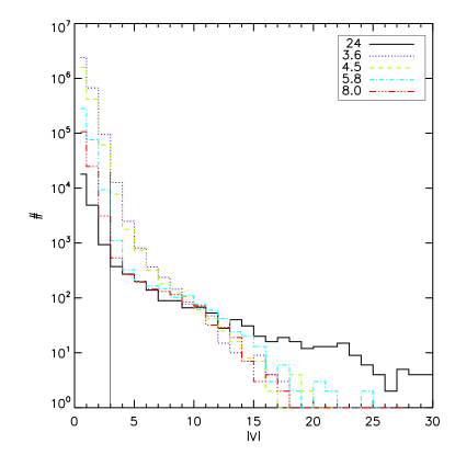
Figure 1: Histogram of all the SAGE sources matched between 2 epochs for the different bands of IRAC and MIPS 24 µm band. Sources with $|V|>$ 3 in at least 2 consecutive bands are classified as variable sources.

2.2 Variability Criteria

Our criterion for a variable source is $|V|>3$ in at least 2 consecutive bands in the same direction. The IRAC-selected sources were matched with the inter-epoch matched 24 µm sources. 24 µm sources with $|V_{24}|>3$ as well as $|V_{8.0}|>3$ in the same direction are deemed 24 µm variables. Table 1 explains the criteria used to identify the variable sources. The first part of the table characterizes the source catalogs. For each band the number of sources with valid fluxes in the band at both epochs, the number and percentage of sources having $|V_{band}|>3$, and the number and percentage of sources expected statistically to have $|V_{band}|>3$ are given. The second part describes the selection criteria and the statistical significance of the variable sources. Here for each band, the sources not only have valid fluxes in both epochs for a given band but also in a neighboring band. Once again the numbers and percentages of sources both meeting the variability criterion and those that might do so based purely on statistical considerations (and therefore likely to be false variables) are given. Assuming that the measurement of flux for any source follows a gaussian distribution characterized by the error in the flux, the probability that two measurements of the flux of a non-variable source will not be within 3-sigma of each other is 0.27%. This applies for every band. We see that for all bands the number of sources with $|V|>3$ is more than that expected from statistical variations. Requiring that the sources have $|V|>$ 3 in at least two bands in the same direction considerably reduces the chances of random mis-classification as a variable source. Firstly a source has to have valid fluxes at both epochs in at least two neighboring bands, and secondly have $|V|>3$ in both of these bands in the same direction. Statistically this has a probability of 0.0004% for bands with a single neighboring band and 0.0007% for bands with two neighbors. For example, at 24 µm less than 1 source would be classified as a variable source due to random chance alone. The argument could be made that the flux measurement of sources does not follow a gaussian distribution, but this simple, idealized statistical approach gives us lower limits on the number of false variables in the list. We perform other tests on the variable source list that do not rely on normal error distributions and uncorrelated errors, and those tests suggest that most of the sources in the list are really variables. A few sources have band-to-band inconsistencies in $V$, that indicates wrong photometry in one band. However, in these cases the the inconsistent band is not responsible for the variability criterion and these fluxes have been nulled in the tables. Of the $\sim 4$ million sources in the SAGE Catalog, Table 2 catalogs the properties (coordinates, fluxes and variability) of the 1,967 SAGE variables.

Table 1: Criteria for variable sources

Criteria	3.6 µm	4.5 µm	5.8 µm	8.0 µm	24 µm
# of sources with valid fluxes	2,962,938	1,939,173	354,290	133,655	25,412
# with $|V_{band}|>$ 3	15341	9857	2395	1647	1625
% with $|V_{band}|>$ 3	0.52	0.51	0.68	1.23	6.39
# expected statistically	8000	5236	957	361	69
% expected statistically	0.27	0.27	0.27	0.27	0.27
# of sources with valid fluxes
in neighboring bands	1,787,038	2,121,027	458,607	124,618	13901
# meet variability criterion	1520	1827	1582	1316	623
% meet variability criterion	0.09	0.09	0.34	1.06	4.48
# expected statistically	8	15	3	$<$1	$<$1
% expected statistically	0.0004	0.0007	0.0007	0.0004	0.0004

Table 2: Properties of the 1967 SAGE Variables

IRAC	MIPS		R.A.	DECL.		3.6 µm				4.5 µm				5.8 µm				8.0 µm				24 µm
Designation	Designation	E	(deg)	(deg)	Class	flux	err	V	fF	… same columns …
						(mJy)	(mJy)
SSTISAGE1C …	SSTM1SAGE1 …	1	79.9337	-69.9940	X	108.80	5.08	4.1	0.25
SSTISAGE2C …	SSTM1SAGE2 …	2	79.9335	-69.9941		85.05	2.71
SSTISAGE1C …	SSTM1SAGE1 …	1	79.9421	-68.8979	Y	0.72	0.04	-4.4	-0.29
SSTISAGE2C …	SSTM1SAGE2 …	2	79.9422	-68.8979		0.96	0.04
SSTISAGE1C …	…	1	79.9643	-72.6359	U	4.93	0.18	-5.4	-0.29
SSTISAGE2C …	…	2	79.9646	-72.6359		3.67	0.15
SSTISAGE1C …	…	1	79.9718	-69.6882	O	5.23	0.18	5.0	0.29
SSTISAGE2C …	…	2	79.9719	-69.6883		6.97	0.30
SSTISAGE1C …	…	1	79.9811	-69.3925	C	25.27	0.63	3.3	0.10
SSTISAGE2C …	…	2	79.9813	-69.3925		22.83	0.39

Note. — Table 2 is published in its entirety in the electronic edition of the Astronomical Journal. A portion is shown here for guidance regarding its form and content.

3 Source Classification

Using the variability criteria discussed in §2 we find $1,967$ SAGE variables at IRAC and MIPS 24 µm bands. 514 sources are variable ($|V|>3$) in all the five bands. Table 2 lists the properties of the 1,967 SAGE variables.

Most of the SAGE variables can be classified as AGB stars, a small number as YSOs and a number of sources that are presently unclassified but could be OB stars, RGB stars, post-AGB stars, PNe, background active galaxies or other classes of variables like cepheids, RR Lyrae stars or WR stars. We choose three color-magnitude diagrams (CMDs) to classify the SAGE variable sources. In Figure 2 all the sources in the SAGE epoch 1 catalog are used to plot the Hess diagram shown in grayscale. Blum et al. (2006) showed that the [J] - [3.6] vs. [3.6] CMD was most useful to see the separation of the O-rich, C-rich and extreme-AGB population. Over-plotted are the epoch 1 magnitudes of the SAGE variable sources classified into O-rich, C-rich and extreme AGBs based on the classification scheme of Cioni et al. (2006) and Blum et al. (2006). The features in the underlying CMD (grayscale) are labeled ‘A’, ‘B’, and ‘C’ (see Blum et al., 2006; Nikolaev & Weinberg, 2000): ‘A’ being the OB star locus at the bluest, faint end of the diagram. The first prominent finger (labeled ‘B’) corresponds to young A-G supergiants (SGs). The finger ‘C’ consists mainly of foreground dwarfs and giants. The next finger to the right in the figure represents late-type(mostly M) SGs and luminous, O-rich M stars (Blum et al., 2006). The rest of the region above the tip of the RGB are divided into O-rich, C-rich and extreme AGB zones. Keeping these divisions in mind lets us classify most of the variable sources as evolved stars. To identify the YSO population, we cross-correlate the variable sources with the SAGE-YSO list from Whitney et al. (2008) and find 29 YSO candidates. Sources that are not classified as evolved stars or YSO candidates are plotted in yellow and will be discussed further in § 3.1.

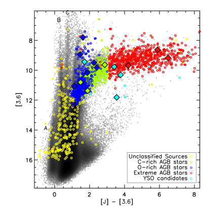
Figure 2: Color magnitude diagrams (CMDs) of the sources detected as variables in the SAGE survey. The SAGE variables over-plotted on a Hess diagram showing the distribution of all the stars in the SAGE Epoch 1 catalog. AGB stars are classified into C-rich, O-rich and extreme AGB following the scheme followed by Cioni et al. 2006 and Blum et al. 2006. YSO candidates are from cross-correlation with the SAGE-YSOs classified by Whitney et al (2008). SEDs of sources plotted with solid diamonds are shown in Figures 7-9 &11.

Meixner et al. (2006) showed that the [8.0] -[24] vs [8.0] CMD was most appropriate for separating the dusty objects based on mass loss. Figure 3 shows the [8.0] - [24] vs [8.0] CMD for the SAGE variables, with the same color-scheme used for the classification as in Figure 2. Figure 4 shows the [4.5] - [24] vs [24] CMD for the SAGE variables. This CMD is the one of the most useful ones to delineate the LMC stellar population from the background population. We see that most of the unclassified sources are among the redder and fainter population in this CMD and are likely to be external galaxies. These sources are further discussed in the next section § 3.1.

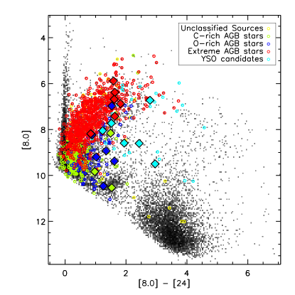
Figure 3: CMD of the SAGE variable sources. Classification of the AGB stars and underlying Hess diagram are same as that in the previous figure. SEDs of sources plotted with solid diamonds are shown in Figures 7-9 &11.

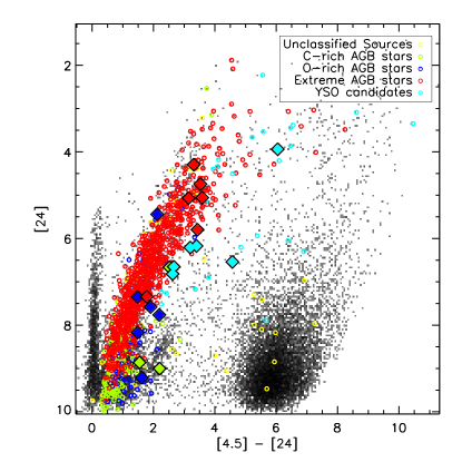
Figure 4: CMD of the SAGE variable sources. Classification of the AGB stars and underlying Hess diagram are same as that in the previous figure. SEDs of sources plotted with solid diamonds are shown in Figures 7-9 &11.

3.1 Unclassified Sources

Using 2MASS and 3.6 µm  color criteria most of the variable sources are classified as evolved AGB stars (with O-rich, C-rich and extreme subclasses). Using the Whitney et al. (2008) YSO candidate list we also identify YSO candidates as infrared variables. The classification of the variable sources that do not fall under any of these subcategories is more challenging. Approximately 17% of the variables remain unclassified and $\sim~{}70\%$ of them remain so mainly because they are missing IRAC and/or 2MASS fluxes. This could be because a) they are undetected being dust enshrouded, e.g very dusty YSOs, b) extremely bright and therefore saturated in IRAC, or c) spatially extended at IRAC wavelengths and thus missing from the point source catalog. In preliminary follow-up work we have identified 20 unclassified sources as cepheids detected in the MACHO survey. Some of the other ‘unclassified’ variables fall on distinct regions of the CMD and could be variable OB stars, RGB stars or O-rich stars that were too faint to be detected in the 2MASS survey. The other sources could be YSOs, Post-AGB sources, PNe, background galaxies or other classes of variables like cepheids, RRLyrae stars, WR stars, QSOs or AGN. Further follow-up work is be required to identify the specific nature of these sources.

4 Discussion

In this first paper we identify infrared variable sources in the LMC and provide an approximate classification as to their nature as discussed in §3. In this section, we discuss the nature of these sources and some implications of their infrared variability for SAGE studies. In particular, we focus on the evolved AGB star population and YSO candidates. The total number of variables identified as SAGE variables is 1,967 or $\sim$0.06% of the $\sim$3 million IRAC point sources that are common to both epoch 1 and 2 catalogs . These fractional numbers suggest that we preferentially detect as variable the redder or dustier sources which tend to be AGB stars or YSOs. In Table 3 we summarize the different categories of sources we have detected as variables and compare them to other work done on the classification of SAGE sources as evolved stars (Blum et al., 2006) and YSO candidates (Whitney et al., 2008) and discuss them below. Histograms (Figure 5) of average variability over all bands show how the AGB stars, YSOs and unclassified sources differ in their variability.

Table 3: SAGE Variable Population

Source Type	SAGE Variables	SAGE Epoch 1 Sources	% detected as variable
Total	1967	4,338,548	0.05
O-rich AGB	353	17,875	1.975
C-rich AGB	426	6,935	6.14
Extreme AGB	820	1,240	66.1
YSO candidate	29	990	2.93
Unclassified	335	4,311,508	0.008

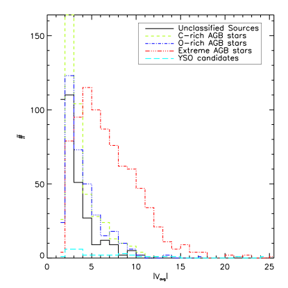
Figure 5: Histogram showing the variability distribution among the different classes of SAGE IRAC variables. Average variability in all 4 bands of IRAC and MIPS 24 µm band has been plotted. C-rich stars in green, O-rich stars in blue, extreme AGBs in red, YSO candidates in cyan and the unclassified sources in black.

4.1 Evolved stars

As expected, the variable source population is dominated by evolved stars, in particular the AGB stars. The SAGE variables have $>81$% AGB stars, classified as either O-rich, C-rich or extreme AGB stars. The spatial distribution of the SAGE variables, as shown in Figure 6, correlates approximately with the LMC 3.6 µm image which traces predominantly the old stellar population of the LMC (Blum et al., 2006) and supports our identification of the variables as evolved stars. In particular, the highest density of sources is located in the main stellar bar of the LMC. The color coding of the point sources on this image follows that of the CMDs. The extreme AGB stars, shown in red, dominate both the spatial distribution of variable sources and the CMDs (Figures 2 – 4). Looking at the numbers of sources detected per category (Table 3) we find that the extreme AGB stars outnumber the O-rich or C-rich AGB stars by a factor of two. Moreover, the percentage of variables changes dramatically across the classified AGB sources. Only 2.0% of the O-rich AGB stars have been detected as variable. This percentage increases to 6.1% for the C-rich AGB stars. For the extreme AGB stars, the percentage jumps to 66%. This increase in percentage follows an evolutionary trend of the AGB. All stars on the early AGB start off as O-rich. As they evolve to higher luminosities their pulsational periods increase, and many become C-rich AGB stars. At the highest luminosities, the periods are the longest and these extreme AGB stars are characterized by significant circumstellar dust emission. Thus, the fractional number of AGB stars identified as variable increases as the star becomes more evolved on the AGB.

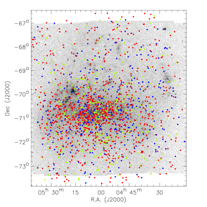
Figure 6: The spatial distribution of the variable sources in the LMC classified as AGB stars plotted on the 3.6 µm map. Note the correlation of the spatial distribution of the variable population with the stellar density function (3.6 µm). This confirms that most of these sources are indeed stars. The colors represent the same classification of the sources as used in Figure 2.

This preferential detection of the evolved AGB stars is similar to that in the IRAS variability studies in our Galaxy because our sampling period of 2 measurements separated by 3 months is similar to the IRAS sampling. As Harmon & Gilmore (1988) found in our Galaxy, we are preferentially finding the more evolved, dusty AGB stars which probably have longer periods. This preference is at least in part due to the sensitivities of detection and of time sampling. Because they are more luminous and dust enshrouded, the extreme AGB stars are easier to detect and their variability is easier to measure reliably in the IRAC and MIPS bands. In addition, the period of the variability for the extreme AGB stars, $\sim$400-500 days, is well matched to our two sample points in time separated by 3 months ($\sim$90 days) such that we could more likely than not measure a detectable flux difference in the two epochs.

Even though we do not detect all the AGB stars as infrared variables, we do know that they are all variables (e.g. Fraser et al., 2005). The detected infrared variability reported here provides a constraint on the possible range of the infrared flux in these types of AGB stars. The fractional difference in fluxes we detect has a range of 0.1 to 1.5 of the total flux. These changes in infrared flux will have significant implications for the analysis of SAGE data on the AGB stars. Estimates of the infrared excesses for this population will have some systematic errors because of the infrared variability. The mass-loss rates of the evolved stars will be derived from model fits to the spectral energy distributions of these sources, and the IRAC and MIPS 24 µm photometry provide constraints on the dusty shells. The infrared variability of the three different classes of AGB stars is revealed in the 2-epoch spectral energy distributions of a few O-rich, C-rich and extreme AGB stars selected from our sample (Figures 7 – 9). The SEDs show the SAGE epoch1 data connected by dotted lines and epoch2 data by dashed lines. The 2MASS data are connected by solid lines and in many instances appears disjoint from either of the epochs, which is due to infrared variability as these data represent a different phase far removed from either of the SAGE epochs. The O-rich and C-rich AGB stars show a similar amount of variation and the extreme AGB star shows a larger variation. Indeed the extreme AGB stars typically have a larger variability index than the O-rich and C-rich AGB stars (Figure 5).

Figure 7: Spectral energy distributions showing the two epochs of a sample of variable O-rich AGB stars. SAGE epoch 1 fluxes are connected by dotted lines and epoch 2 by dashed lines. The sources are marked with solid, blue diamonds on the CMDs. The 2MASS data are connected by solid lines and in many instances appears disjoint from either of the epochs, which is due to infrared variability as these data represent a different phase far removed from either of the SAGE epochs.

Figure 8: Spectral energy distributions showing the two epochs of a sample of variable C-rich AGB stars. The sources are marked as solid, green diamonds on the CMDs. SAGE epoch 1 fluxes are connected by dotted lines and epoch 2 by dashed lines. The sources are marked with solid, red diamonds on the CMDs. The 2MASS data are connected by solid lines and in many instances appears disjoint from either of the epochs, which is due to infrared variability as these data represent a different phase far removed from either of the SAGE epochs.

Figure 9: Spectral energy distributions showing the two epochs of a sample of variable extreme AGB stars. SAGE epoch 1 fluxes are connected by dotted lines and epoch 2 by dashed lines. The sources are marked with solid, red diamonds on the CMDs. The 2MASS data are connected by solid lines and in many instances appears disjoint from either of the epochs, which is due to infrared variability as these data represent a different phase far removed from either of the SAGE epochs.

Some of the brightest variables are not classified because they are saturated in IRAC 3.6 µm  band or 2MASS bands, which we use for classification purposes. The drop in flux in the Raleigh-Jeans tails of the SED enables them to be detected at the longer IRAC bands (4.5, 5.8 and 8.0 µm) and MIPS 24 µm without saturation.

4.2 YSO candidates

We have discovered a YSO candidate population with infrared variability. That this phenomenon was not noticed earlier is not surprising given that little work has been done on infrared variability of YSOs and most of it has been followup of known optically variable sources. These variable YSO candidates comprise at least 3% of all the YSO candidates. We say at least, because there are a large number of sources in the same CMD space that are “unclassified”. The spatial distribution of YSO candidates correlates spatially with the LMC MIPS 24 micron emission, which traces massive star formation, supporting the identification of these variables as YSOs (Figure 10). Also interesting is the spatial distribution of the “unclassified” sources (Figure 10). These sources also closely follow the the 24 µm emission. Further follow up work on extending the list of YSO variables that is in progress will help clarify if some of these unclassified sources are YSOs.

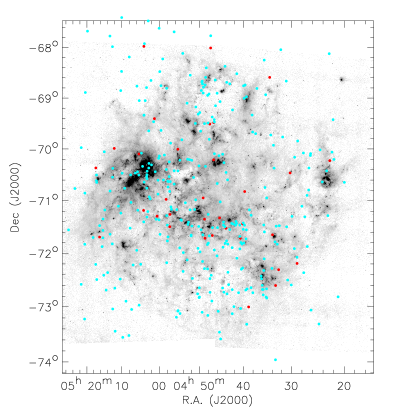
Figure 10: The spatial distribution of variable massive YSOs and the unclassified sources plotted on SAGE 24 µm image. The YSO candidates are shown in red and the unclassified candidates in cyan.

In this study, the variability for this YSO population shows most prominently in the MIPS 24 µm band (24 of 29 YSO candidates have $|V_{24}|>3$). The reason for the predominance of MIPS 24 µm band variability becomes clear when we examine the SEDs of a few variable YSO candidates (Figure 11). The SEDs show the SAGE epoch1 data connected by dotted lines and epoch2 data by dashed lines. The 2MASS data are connected by solid lines and in many instances appears disjoint from either of the epochs, which is due to infrared variability as these data represent a different phase far removed from either of the SAGE epochs. Most of these sources are very faint in the 2MASS and IRAC bands, and increase rapidly in flux at the longer wavelengths. In fact, while our SEDs end at 24 µm  the trend suggests that for some of these YSOs, the SEDs actually peak at even longer wavelengths. Thus, our sensitivity to these sources is greatest at 24 µm and the lower number of IRAC variable YSO candidates in the SAGE data may be due to the lower sensitivity in the IRAC bands to detect the variability.

Figure 11: Spectral energy distributions (SEDs) of a sample of YSO variable sources. The sources are marked as solid, cyan diamonds on the CMDs. SAGE epoch 1 fluxes are connected by dotted lines and epoch 2 by dashed lines. The sources show SEDs consistent with embedded objects with dust emission. The sources are marked with solid, red diamonds on the CMDs. The 2MASS data are connected by solid lines and in many instances appears disjoint from either of the epochs, which is due to infrared variability as these data represent a different phase far removed from either of the SAGE epochs.

Whitney et al. (2008) have completed a candidate list of over 990 YSO candidates identified in the SAGE epoch 1 catalog. This list is a lower limit to the total number of YSOs in the LMC because the selection was conservative and avoided regions in CMD space densely populated by other types of sources, e.g. AGB stars and background galaxies. Our variable YSO candidates comprise $\sim~{}3\%$ of the larger 990 YSO candidate list. It is difficult to assess if this percentage is a lower or upper limit because the number of YSOs and variable YSOs is rather uncertain in different directions. Nevertheless, the percentage is significant enough to catch our attention as a new class of infrared variables. With only two epochs of observation spread 3 months apart, we cannot distinguish between a periodic or a more stochastic phenomenon for the YSOs. Clearly, further study of these sources is required to understand the nature of their variability.

5 Conclusions

We have detected infrared variable stars in the LMC using the SAGE survey. The variable source population is dominated by evolved stars, in particular the AGB stars (81% of the SAGE variables). We preferentially find the more evolved, dusty AGB stars which probably have longer periods. We also present the discovery of a YSO candidate population with infrared variability. These variable YSO candidates comprise about 3% of all the SAGE variables.

References

- Ábrahám et al. (2004) Ábrahám, P., Kóspál, Á., Csizmadia, S., Kun, M., Moór, A., & Prusti, T. 2004, A&A, 428, 89
- Alcock et al. (1996) Alcock, C., et al. 1996, AJ, 111, 1146
- Blum et al. (2006) Blum, R. D. et al. 2006, AJ, 132, 2034
- Cioni et al. (2006) Cioni, M.-R.L., Giardi, L., Marigo, P., & Habing, H. J. 2006, A&A, 448, 77
- Fazio et al. (2004) Fazio, G. G., et al. 2004, ApJS, 154, 39
- Fraser et al. (2005) Fraser, O. J., Hawley, S. L., Cook, K. H., & Keller, S. C. 2005, AJ, 129, 768
- Groenewegen et al. (2007) Groenewegen, M. A. T., et al. 2007, MNRAS, 376, 313
- Harmon & Gilmore (1988) Harmon, R., & Gilmore, G. 1988, MNRAS, 235, 1025
- Hartmann & Kenyon (1985) Hartmann, L., & Kenyon, S. J. 1985, ApJ, 299, 462
- Herbig et al. (2003) Herbig, G. H., Petrov, P. P., & Duemmler, R. 2003, ApJ, 595, 384
- Juhász et al. (2007) Juhász, A., Prusti, T., Ábrahám, P., & Dullemond, C. P. 2007, MNRAS, 374, 1242
- Meixner et al. (2006) Meixner, M. et al. 2006, AJ, 132, 2268
- Natta et al. (1997) Natta, A., Grinin, V. P., Mannings, V., & Ungerechts, H. 1997, ApJ, 491, 885
- Nikolaev & Weinberg (2000) Nikolaev, S., & Weinberg, M. D. 2000, ApJ, 542, 804
- Omont et al. (1999) Omont, A., et al. 1999, A&A, 348, 755
- Paczynski et al. (1994) Paczynski, B., Stanek, K. Z., Udalski, A., Szymanski, M., Kaluzny, J., Kubiak, M., Mateo, M., & Krzeminski, W. 1994, ApJ, 435, L113
- Prusti & Mitskevich (1994) Prusti, T., & Mitskevich, A. S. 1994, ASP Conf. Ser. 62: The Nature and Evolutionary Status of Herbig Ae/Be Stars, 62, 257
- Rieke et al. (2004) Rieke, G. H. et al. 2004, ApJS, 154, 25
- Skrutskie et al. (2006) Skrutskie, M. F., et al. 2006, AJ, 131, 1163
- van der Veen & Habing (1990) van der Veen, W. E. C. J., & Habing, H. J. 1990, A&A, 231, 404
- Werner et al. (2004) Werner, M., et al. 2004, ApJS, 154, 1
- Whitelock et al. (2003) Whitelock, P. A., Feast, M. W., van Loon, J. T., & Zijlstra, A. A. 2003, MNRAS, 342, 86
- Whitney et al. (2008) Whitney, B. A. et al. 2008, AJ, 136, 18
- Zaritsky et al. (2004) Zaritsky, D., Harris, J., Thompson, I. B., & Grebel, E. K. 2004, AJ, 128, 1606