Exact and Asymptotic Conditions on Traveling Wave Solutions of the Navier-Stokes Equations

Abstract

We derive necessary conditions that traveling wave solutions of the Navier-Stokes equations must satisfy in the pipe, Couette, and channel flow geometries. Some conditions are exact and must hold for any traveling wave solution irrespective of the Reynolds number ($Re$). Other conditions are asymptotic in the limit $Re\rightarrow\infty$. The exact conditions are likely to be useful tools in the study of transitional structures. For the pipe flow geometry, we give computations up to $Re=100000$ showing the connection of our asymptotic conditions to critical layers that accompany vortex structures at high $Re$.

Turbulence is sometimes said to be the last unsolved problem of classical physics. However, in a sense it is a fully solved problem, since we know with near certainty that the Navier-Stokes equations (NSE), along with the no-slip boundary conditions Lauga et al. (2007), are an excellent physical model for all the phenomena associated with turbulence and transition.

Although the physical model is known, figuring out the solutions of the NSE has proved to be a very difficult problem, computationally or analytically. To illustrate this difficulty, we note that while useful models of the structural strength of an entire aircraft can be built using $1$ to $100$ million elements, it takes more than a billion grid points to completely resolve the flow in a cubical volume of extent an inch³ at the surface of a car moving at around $60$ m.p.h. Blackwelder and Kaplan (1976); Hoyas and Jiménez (2006); Mukund et al. (2006).

The Navier-Stokes equations, which model the evolution of the velocity field ${\bf u}$ of an incompressible fluid, are $\partial{\bf u}/\partial t+({\bf u}.\nabla){\bf u}=-\nabla p+(1/Re)\triangle{\bf u}$, where the velocity field ${\bf u}$ must satisfy the incompressibility constraint $\nabla.{\bf u}=0$. There is no explicit equation for evolving the pressure $p$, and $Re$ denotes the Reynolds number.

Traveling wave solutions of the form ${\bf u}({\bf x},t)=\tilde{\bf u}(x-{\bf c}t)$ form our main topic. As the motion of turbulent fluids is characterized by disordered and intermittent fluctuations about a mean, the significance of traveling wave solutions may seem limited. Indeed, one has to look at more complicated solutions to begin to understand turbulent fluctuations Viswanath (2007). However, there is gathering evidence that traveling wave solutions may help understand certain coherent structures in transitional pipe flow Schneider et al. (2007); Willis and Kerswell (2008).

Further, using certain lower-branch traveling waves, we can exhibit critical layers at high $Re$ Viswanath (2009); Wang et al. (2007) that are far beyond the reach of ordinary direct numerical simulation. The Orr-Sommerfeld equation, which governs the propagation of infinitesimal normal mode perturbations of a base flow, is singular at $Re=\infty$, which is the origin of the theory of critical layers Maslowe (1981, 1986). The ability to compute critical layers in fully resolved numerical solutions of the NSE could be significant, as critical layers occur in many important situations Maslowe (1986). The gigantic trailing vortices that escape from the boundary layers of airplanes during take-off may develop critical layers Maslowe and Nigam (2008). So could vortices shed by wind turbines, with possible implications for the optimal arrangement of turbines in a wind farm.

Many linearly unstable (and non-laminar) traveling wave solutions and equilibria (which are special cases with ${\bf c}=0$) of Couette Nagata (1990, 1997), channel Waleffe (1998, 2003), and pipe Faisst and Eckhardt (2003); Wedin and Kerswell (2004) geometries have been computed. A notably systematic and extensive effort is due to Gibson and others Gibson et al. (2008, 2009). The exact conditions we derive must hold for the velocity fields of all these solutions. In addition, analogous conditions must hold for periodic solutions and relative periodic solutions that travel only in the streamwise direction.

The mere existence of traveling wave solutions does not imply their relevance to phenomena as they manifest themselves in Nature and in technology. However, efforts to connect traveling waves computed in short pipes to puffs have been partially successful Schneider et al. (2007); Willis and Kerswell (2008). Puffs are transitional structures observed in pipes around $Re=2000$ that are approximately $20$ pipe diameters in axial length and which travel with a speed that is somewhat less than the mean streamwise velocity Peixinho and Mullin (2006). Tantalizingly, there are hints that an entire puff may correspond to a traveling wave or some such solution of pipe flow Willis and Kerswell (2009). Our exact conditions will be helpful in the investigation of that possibility.

We now turn to the derivation of the exact conditions. In the velocity field ${\bf u}=(u,v,w)$ of the NSE, $u$, $v$ and $w$ are the streamwise (coordinate axis $x$), wall-normal ($y$), and spanwise ($z$) components, respectively, for the rectangular Couette and channel geometries. In the case of pipe flow, $u$, $v$ and $w$ are the radial ($r$), polar ($\theta$) and streamwise (or axial) ($z$) components, respectively.

In plane Couette flow, the walls at $y=\pm 1$ move in the $x$ direction with speeds equal to $\pm 1$. The boundary conditions in the streamwise and spanwise directions are periodic, with the periods taken to be $2\pi\Lambda_{x}$ and $2\pi\Lambda_{z}$, respectively. For pipe flow, we assume the axial or streamwise boundary condition to be periodic with period $2\pi\Lambda$. The walls are no slip in all cases. The derivations are given mainly for the plane Couette flow geometry.

Let ${\bf u}({\bf x},t)=\tilde{\bf u}({\bf x}-{\bf c}t)$ be a traveling wave solution of plane Couette flow. We assume ${\bf c}=(c,0,0)$ so that the traveling wave moves in the streamwise direction only. If $\tilde{\bf u}=(u,v,w)$, the streamwise or $x$ component of the NSE gives

$$-c{\partial_{x}u}+\bigl{(}u{\partial_{x}u}+v{\partial_{y}u}+w{\partial_{z}u}\bigr{)}=-{\partial_{x}p}+{c_{p}\over Re}+{1\over Re}\triangle u.$$ (1)

Here $c_{p}/Re$ gives the pressure gradient in the streamwise directions, with $c_{p}=0$ for plane Couette flow and $c_{p}>0$ for channel flow. Let $U(y,z)$ denote $(2\pi\Lambda_{x})^{-1}\int_{0}^{2\pi\Lambda_{x}}u(x,y,z)\,dx$, which is the mean streamwise component of $u$. From (1), we get

$$\overline{\bigl{(}u{\partial_{x}u}+v{\partial_{y}u}+w{\partial_{z}u}\bigr{)}}={c_{p}+\triangle U\over Re},$$ (2)

where the overline denotes streamwise averaging. At the walls $y=\pm 1$, ${\partial_{x}u}=0$ and $v=w=0$ because of no-slip. For the same reason, ${\partial_{zz}U}=0$ at the walls. Therefore,

$$c_{p}+{\partial_{yy}U}=0$$ (3)

must hold at the walls.

As the velocity field $\tilde{\bf u}$ has zero divergence, we may rewrite (2) as

$$\overline{\nabla\cdot(u^{2},uv,uw)}={\partial_{y}\overline{uv}}+{\partial_{z}\overline{uw}}={c_{p}+\triangle U\over Re}.$$ (4)

If (4) is integrated over the cross-section, Green’s theorem applies to the expression in the middle of (4). The integral of the middle term must be zero because $v=0$ at the walls and $uw$ is periodic in $z$. Thus we have

$$\int_{0}^{2\pi\Lambda_{z}}\int_{-1}^{+1}(\triangle U+c_{p})\,dy\,dz=0.$$ (5)

The derivation of the necessary conditions (3) and (5) applies to channel flow with no change. However, $c_{p}\neq 0$ for channel flow.

The conditions (3) and (5) must be satisfied by all traveling wave solutions of plane Couette flow or channel flow, whose wave speed vector ${\bf c}$ only has a streamwise component. Indeed, those conditions must be satisfied by all periodic solutions ${\bf u}({\bf x},t)={\bf u}({\bf x},t+T)$, $T$ being the period, or relative periodic solutions ${\bf u}({\bf x},t)={\bf u}({\bf x+s},t+T)$ if the shift ${\bf s}$ only has a streamwise component. To form $U$ in those instances, one must average both over a single period and in the streamwise direction as a simple modification of our derivation will show.

For the case of pipe flow, let ${\bf c}=(0,0,c)$ so that the traveling wave travels in the streamwise direction only. Let $W(r,\theta)=(2\pi\Lambda)^{-1}\int_{0}^{2\pi\Lambda}w(r,\theta,z)\,dz$ be the mean streamwise velocity. The analogue of (3) requires

$$c_{p}+\partial_{r}^{2}W+{\partial_{r}W\over r}=0$$ (6)

at all points on the circumference. If we assume the pipe radius to be $1$, the analogue of (5) is

$$\int_{0}^{2\pi}\int_{0}^{1}(\triangle W+c_{p})r\,dr\,d\theta=0.$$ (7)

The derivation of the necessary conditions (6) and (7) for pipe flow is similar to that of their Couette analogues.

Traveling waves normally arise from saddle-node bifurcations with increasing $Re$ Nagata (1990); Waleffe (1998); Schmiegel (1999); Faisst and Eckhardt (2003); Wedin and Kerswell (2004). The branch corresponding to lower energy dissipation is called the lower branch. We will now derive certain scalings with respect to increasing $Re$ that are characteristic of the lower branch families.

In the case of plane Couette flow or channel flow, if a traveling wave solution is given by $\tilde{\bf u}({\bf x}-{\bf c}t)$, the velocity field $\tilde{\bf u}({\bf x})$ can be decomposed as

$${\bf u}_{0}(y,z)+\sum_{n=1}^{\infty}\bigl{(}{\bf u}_{n}(y,z)\exp(i\alpha x)+\text{c.c}\bigr{)},$$ (8)

where $\alpha=1/\Lambda_{x}$. We take ${\bf u}_{0}=(U,v_{0},w_{0})$ and ${\bf u}_{i}=(u_{i},v_{i},w_{i})$ for $i\geq 1$. For pipe flow, the decomposition analogous to (8) is given by ${\bf u}_{0}(r,\theta)+\sum_{n=1}^{\infty}\bigl{(}{\bf u}_{n}(r,\theta)\exp(i\alpha z)+\text{c.c}\bigr{)}$, with $\alpha=1/\Lambda$. We take ${\bf u}_{i}=(u_{i},v_{i},w_{i})$ for $i\geq 1$ as for Couette flow, but ${\bf u}_{0}=(u_{0},v_{0},W)$ for pipe flow.

The scalings of the lower branch family that are known or that will be derived apply to the mean streamwise velocity ($U$ or $W$), or the rolls ($(v_{0},w_{0})$ or $(u_{0},v_{0})$), or the magnitude of modes such as ${\bf u}_{1}$. It is an empirical fact (but see Waleffe (1997); Wedin and Kerswell (2004); Lundbladh et al. (1994)) that the rolls and the $\bf{u}_{1}$ mode diminish in magnitude approximately at the rate $Re^{-1}$. Higher modes with $n>1$ appear to diminish even faster. The derivations assume these scalings. In addition, the dissipation rate of the lower branch families decrease with increasing $Re$, assuming that the dissipation rate of the laminar solution is normalized to be $1$ Viswanath (2009); Wang et al. (2007).

The wall-normal or $y$ component of the $n=1$ mode of the NSE gives

$$i\alpha(U-c)v_{1}=-\partial_{y}p_{1}+Re^{-1}(-\alpha^{2}v_{1}+\partial_{y}^{2}v_{1}+\partial_{z}^{2}v_{1})+\cdots$$ (9)

for plane Couette or channel flow. The first neglected terms in (9) are $-v_{0}\partial_{y}v_{1}-w_{0}\partial_{z}v_{1}-v_{1}\partial_{y}v_{0}-w_{1}\partial_{z}v_{0}$. The analogous equation for the radial component of pipe flow is $i\alpha(W-c)u_{1}=-\partial_{r}p_{1}+Re^{-1}\triangle_{r}u_{1}$, where $\triangle_{r}$ corresponds to the usual form of the Laplacian in the radial component of the NSE. Terms such as $-v_{1}\partial_{\theta}v_{0}/r$ are neglected.

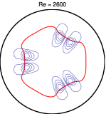
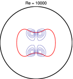
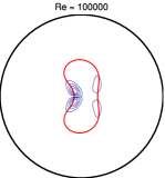
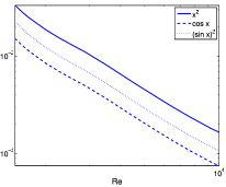
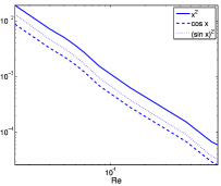
Figure 1: Three traveling wave solutions of pipe flow are shown. Units are chosen to make the pipe radius and the centerline speed of the laminar solution equal to $1$. The boundary condition fixes the mass flux (and not the pressure gradient) to be that of the laminar solution. Solutions (a) and (b) correspond to the $c$ family and the upper dash-dot curve of Figure 7 of Wedin and Kerswell (2004), respectively. For more on (c), see Viswanath (2009). In the upper plots, the four contour levels of $\lvert u_{1}\rvert$ are equispaced in $(0,{\rm max})$, with max being $.0094$, $.0011$, and $.0002$, respectively. The thick line is the critical curve. The plots below correspond to the ones directly above. Plot (d) (the thick line is for $c_{p}$) can be validated against Figure 7 of Wedin and Kerswell (2004) after replacing $Re$ and $c$ by $c_{p}\,Re$ and $c/c_{p}$, respectively. In (e) and (f), the legends show the choice of $f(x)$ and the curves illustrate (14) ($\alpha\approx 1.5$).

Using (9), Waleffe et al.Wang et al. (2007) estimated that most of the variation in $v_{1}$ is concentrated in a region around the critical curve $U=c$, with the width of that region scaling as $Re^{-1/3}$. In the case of pipe flow, an identical argument gives $W=c$ as the equation of the critical curve. The top set of plots in Figure 1 illustrate the critical layer in the case of pipe flow.

To derive further scalings, we consider the streamwise component of the $n=0$ mode of NSE, which is

$$v_{0}\partial_{y}U+w_{0}\partial_{z}U=Re^{-1}(c_{p}+\triangle U)+M$$ (10)

for plane Couette or channel flow. The pipe flow analogue is $u_{0}\partial_{r}W+(v_{0}/r)\partial_{\theta}W=Re^{-1}(c_{p}+\triangle W)+M$. In (10) and its pipe flow analogue, $-M$ equals the $n=0$ mode of the streamwise component of $((\tilde{\bf u}-{\bf u}_{0}).\nabla)(\tilde{\bf u}-{\bf u}_{0})$. From here on we restrict the derivation to plane Couette flow or to channel flow.

Since ${\bf u}_{0}=(U,v_{0},w_{0})$ has zero divergence, we can find a function $\psi(y,z)$ such that $v_{0}=\partial_{z}\psi$ and $w_{0}=-\partial_{y}\psi$. We then get

$$L\psi=Re^{-1}(c_{p}+\triangle U)+M,$$ (11)

where

$$L=(\partial_{y}U)\,\,\partial_{z}-(\partial_{z}U)\,\,\partial_{y}.$$ (12)

The skew-symmetry of the linear operator $L$ is the key to deducing further scalings. The skew-symmetry of $L$ is likely to be important in attempts to find an asymptotic theory for the critical layer.

Let $\phi(y,z)$ and $\psi(y,z)$ have $z$ periods of $2\pi\Lambda_{z}$ and be sufficiently smooth. The following calculation uses integration by parts:

$$\int_{0}^{2\pi\Lambda}\int_{-1}^{1}\phi L\psi\,dy\,dz=\int_{-1}^{1}\phi\psi U_{y}\bigl{\lvert}_{0}^{2\pi\Lambda}dy$$

$$-\int_{0}^{2\pi\Lambda}\int_{-1}^{1}(\psi U_{y}\phi_{z}+\psi\phi U_{yz})dy\,dz-\int_{0}^{2\pi\Lambda}\phi\psi U_{z}\bigl{\lvert}_{-1}^{1}dz$$

$$+\int_{0}^{2\pi\Lambda}\int_{-1}^{1}(\psi U_{z}\phi_{y}+\psi\phi U_{yz})dy\,dz,$$

where the subscripts are for partial derivatives. On the right hand side, two double integral terms cancel and the single integral terms are both zero because $U_{y}$ is periodic in $z$ and $U_{z}$ is zero at the walls (from no-slip). We are left with $-\int\int\psi L\phi\,dy\,dz$ on the right, verifying skew-symmetry of the operator $L$.

From direct substitution into (12), it is evident that $L(f(U))=0$ for any smooth $f$. Thus the functions $f(U)$ are in the kernel of the anti-symmetric operator $L$. Since the linear system (11) can be solved for $\psi$ (or equivalently for the rolls), the Fredholm alternative implies that

$$\int_{0}^{2\pi\Lambda_{z}}\int_{-1}^{1}f(U)\bigl{(}c_{p}+\triangle U+Re\,M\bigr{)}\,dy\,dz=0.$$

For lower-branch traveling wave families with $\tilde{\bf u}-{\bf u}_{0}$ of magnitude $Re^{-\alpha}$ with $\alpha\approx 1$, the magnitude of $M$ is approximately $Re^{-2}$ in the limit $Re\rightarrow\infty$. We have

$$\int f(U)\Bigl{(}\triangle U(y,z)+c_{p}\Bigr{)}dy\,dz=O(Re^{-\alpha})$$ (13)

for any smooth $f$. Here $\alpha>1$ is possible if there are cancellations in the integral of $M$ over the cross-section. The analogous condition for pipe flow is given by

$$\int f(W)\Bigl{(}\triangle W(r,\theta)+c_{p}\Bigr{)}rdr\,d\theta=O(Re^{-\alpha})$$ (14)

with $\alpha$ as above.

In addition to the pipe families of Figure 1, we computed a lower branch equilibrium family and a traveling wave family up to $Re=45000$ and $Re=7000$. The (a) and (b) families of Figure 1 could not be continued to $Re$ much higher than shown in the top plots. For a given resolution, we cannot expect to find solutions if the rolls, which diminish in magnitude with $Re$, are too small to be detected. Even after using sufficient resolution, the GMRES-hookstep iterations (see Viswanath (2007, 2009)) became very slow. Even though the residual error could be made quite small, the norm of the Newton steps became quite large and increased with iteration. Although it is uncertain if the lower branch families exist in the $Re\rightarrow\infty$ limit, Figure 1 amply demonstrates that they exist for large enough $Re$ for the predicted scalings to hold.

The critical curves are away from the pipe walls and have an inward indentation where the counter-rotating vortices face each other. Since the critical behavior is evident even for $Re=2600$, we suspect that critical curves or surfaces may give a way to visualize the structure of puffs in transitional pipe flow.

In summary, we have given a number of necessary conditions for equilibrium, traveling wave, periodic, and relative periodic solutions in plane Couette, channel and pipe geometries. We have argued for the importance of critical layers in high $Re$ fluid flow and shown the connection of our analysis to critical layers. In addition, the conditions that we have derived are likely to be useful in the study of transitional structures such as puffs in pipe flow.

References

- Lauga et al. (2007) E. Lauga, M. Brenner, and H. Stone, in Springer Handbook of Experimental Fluid Mechanics (Springer, Berlin, 2007), chap. 19, pp. 1219–1240.
- Blackwelder and Kaplan (1976) R. Blackwelder and R. Kaplan, Journal of Fluid Mechanics 76, 89 (1976).
- Hoyas and Jiménez (2006) S. Hoyas and J. Jiménez, Physics of Fluids 18, 011702:1 (2006).
- Mukund et al. (2006) R. Mukund, P. Viswanath, R. Narasimha, A. Prabhu, and J. Crouch, Journal of Fluid Mechanics 566, 97 (2006).
- Viswanath (2007) D. Viswanath, Journal of Fluid Mechanics 580, 339 (2007).
- Schneider et al. (2007) T. Schneider, B. Eckhardt, and J. Vollmer, Physical Review E 75, 066313 (2007).
- Willis and Kerswell (2008) A. Willis and R. Kerswell, Physical Review Letters 100, 124501 (2008).
- Viswanath (2009) D. Viswanath, Philosophical Transactions of the Royal Society A 367, 561 (2009).
- Wang et al. (2007) J. Wang, J. Gibson, and F. Waleffe, Physical Review Letters 98, 204501 (2007).
- Maslowe (1981) S. Maslowe, in Hydrodynamic Instabilities and the Transition to Turbulence, edited by H. Swinney and J. Gollub (Springer-Verlag, 1981), pp. 181–228.
- Maslowe (1986) S. Maslowe, Annual Reviews in Fluid Mechanics 18, 405 (1986).
- Maslowe and Nigam (2008) S. Maslowe and N. Nigam, SIAM Journal of Applied Mathematics 68, 825 (2008).
- Nagata (1990) M. Nagata, Journal of Fluid Mechanics 217, 519 (1990).
- Nagata (1997) M. Nagata, Physical Review E 55, 2023 (1997).
- Waleffe (1998) F. Waleffe, Physical Review Letters 81, 4140 (1998).
- Waleffe (2003) F. Waleffe, Physics of Fluids 15, 1517 (2003).
- Faisst and Eckhardt (2003) H. Faisst and B. Eckhardt, Physical Review Letters 91, 224502 (2003).
- Wedin and Kerswell (2004) H. Wedin and R. Kerswell, Journal of Fluid Mechanics 508, 333 (2004).
- Gibson et al. (2008) J. Gibson, J. Halcrow, and P. Cvitanović, Journal of Fluid Mechanics 611, 107 (2008).
- Gibson et al. (2009) J. Gibson, J. Halcrow, and P. Cvitanović, Journal of Fluid Mechanics (2009), to appear.
- Peixinho and Mullin (2006) J. Peixinho and T. Mullin, Physical Review Letters 96, 094501 (2006).
- Willis and Kerswell (2009) A. Willis and R. Kerswell, Journal of Fluid Mechanics 619, 213 (2009).
- Schmiegel (1999) A. Schmiegel, Ph.D. thesis, Philipps-Universitát Marburg (1999).
- Waleffe (1997) F. Waleffe, Physics of Fluids 9, 883 (1997).
- Lundbladh et al. (1994) A. Lundbladh, D. Henningson, and S. Reddy, in Turbulence and Combustion, edited by M. Hussaini, T. Gatski, and T. Jackson (Kluwer, Holland, 1994).