Gaseous drag on a gravitational perturber in Modified Newtonian Dynamics and the structure of the wake

Abstract

We calculate the structure of a wake generated by, and the dynamical friction force on, a gravitational perturber travelling through a gaseous medium of uniform density and constant background acceleration $\mn@boldsymbol{g}_{\rm ext}$, in the context of Modified Newtonian Dynamics (MOND). The wake is described as a linear superposition of two terms. The dominant part displays the same structure as the wake generated in Newtonian gravity scaled up by a factor $\mu^{-1}(g_{\rm ext}/a_{0})$, where $a_{0}$ is the constant MOND acceleration and $\mu$ the interpolating function. The structure of the second term depends greatly on the angle between $\mn@boldsymbol{g}_{\rm ext}$ and and the velocity of the perturber. We evaluate the dynamical drag force numerically and compare our MOND results with the Newtonian case. We mention the relevance of our calculations to orbit evolution of globular clusters and satellites in a gaseous proto-galaxy. Potential differences in the X-ray emission of gravitational galactic wakes in MOND and in Newtonian gravity with a dark halo are highlighted.

1 Introduction

According to the Brownian theory, a ‘macroscopic’ particle moving in a fluid experiences a fluctuating force as a consequence of the graininess of the fluid, resulting in dynamical friction (DF) and diffusion in the velocity-space. Understanding the nature of the DF force experienced by a gravitational object that moves against a mass density background is of great importance for describing the evolution of gravitational systems and the exchange of angular and linear momentum between gravitational subsystems. There are two limits of interest in astrophysics: pure collisionless media and fully collisional gas. If the pertuber only interacts with the surrounding particles gravitationally, either the medium is collisionless or collisional, the DF force is the result of the formation of an overdensity wake behind the perturber.

The DF depends on the nature of the force between the perturber and the background particles. Departures from Newtonian gravity have been proposed as an alternative to dark matter in galaxies (e.g., Modified Newtonian Dynamics; Milgrom 1983). Ciotti & Binney (2004) found that in collisionless backgrounds, the characteristic timescale for DF in Modified Newtonian Dynamics (MOND) is much shorter than in the Newtonian equivalent system with dark matter. If confirmed, this result may have strong astrophysical implications and may be used to distinguish between dark matter and modified gravity. Using the MOND scaling found in Ciotti & Binney (2004), the globular clusters in Fornax dwarf spheroidal galaxy should have spiraled into the centre of Fornax in $\sim 0.5$ Gyr, forming a visible galactic nucleus (Sánchez-Salcedo et al. 2006).

Ciotti & Binney (2004) derived the MOND DF timescale in a restrictive plane-parallel geometry, which is a too specialized case, and in a non-standard statistical formulation. These caveats led Nipoti et al. (2008) to carry out fully N-body simulations of the dynamics of bars in MOND systems. Their simulations confirmed the scaling of the DF timescale predicted in Ciotti & Binney (2004). Still, it is not entirely clear how the background responds to the perturbation, and the description of the structure of the density wake induced by a small and massive perturber is lacking. Since MOND is a nonlinear theory, the gravitational acceleration induced by the perturber is affected by the presence of an external gravitational field. In particular, the DF force is expected to depend on the angle between the direction of the mean field and the velocity of the perturber. Our aim is to understand the nature of DF in MOND.

In this paper we consider gaseous media and study the structure of the density wake induced by a gravitational perturber in MOND. Gaseous DF has found many applications in astrophysics, ranging from protoplanet accretion all the way to the motion of galaxies in clusters (e.g., Ostriker 1999; Kim 2007; Conroy & Ostriker 2008). In a pure baryonic universe as in MOND theory, the relative role of gas becomes even more important because all the contribution to the mass is accounted for by the gas and the stars. Moreover, the complementary view of hydrodynamics may provide new insights into the differences and analogies between Newtonian and modified gravities. Although the details on the internal density structure of the induced wake may depend on whether the system is fully collisional or collisionless, the fluid limit is useful for understanding the main conceptual features introduced by the change of the gravity law.

The linear response of the gaseous medium to a gravitational perturber in Newtonian gravity is well-documented (Dokuchaev 1964; Ruderman & Spiegel 1971; Just & Kegel 1990; Ostriker 1999; Sánchez-Salcedo & Brandenburg 1999, 2001; Kim & Kim 2007; Kim et al. 2008). In all these works, a minimum radius $r_{\rm min}$ in the Coulomb logarithm was introduced in order to regularise the gravitational potential of a point mass. Although the formulae were derived for rectilinear orbits in homogeneous and infinity media, simple ‘local’ extensions have been proven very successful in more realistic situations, e.g., smoothly decaying density backgrounds or when the perturber is moving on a circular orbit (Sánchez-Salcedo & Brandenburg 2001; Kim & Kim 2007).

The paper is organized as follows. In §2, we discuss the basic concepts on the ideal problem of a point particle moving at constant speed within a uniform gas in MOND (the Bondi-Hoyle problem). In §3, we outline the linear derivation of the basic equations for calculating the steady-state density wake generated by an extended body. In §4 we describe the structure of the resulting wake and evaluate the DF force exerted on the perturber. We then discuss some implications of our results in §5. Finally, we conclude in §6.

2 The Bondy-Hoyle problem in MOND

We consider a gravitational point particle at the origin of our coordinate system, surrounded by a gas whose velocity far from the particle is

$$\mn@boldsymbol{v}_{\infty}={\mathcal{M}}c_{\infty}\hat{z},$$ (1)

where $c_{\infty}$ is the sound speed of the gas at infinity and ${\mathcal{M}}$ is the Mach number. We are interested in the wake produced by the gravitational interaction with the perturber in the context of MOND.

Bekenstein & Milgrom (1984) suggested a Lagrangian theory and also a nonlinear differential equation for the nonrelativistic MOND gravitational potential produced by a mass density distribution $\rho$:

$$\mn@boldsymbol{\nabla}\cdot\left[\mu\left(\frac{|\mn@boldsymbol{\nabla}\Phi|}{a_{0}}\right)\mn@boldsymbol{\nabla}\Phi\right]=4\pi G\rho,$$ (2)

where $a_{0}\sim 10^{-8}$ cm s^-2 is an universal acceleration and $\mu(x)$ is a monotonic and continuous function with the property that $\mu(x)\simeq x$ for $x\ll 1$ (deep MOND regime) and $\mu(x)\simeq 1$ for $x\gg 1$ (Newtonian regime). Only for very special configurations (one-dimensional symmetry –spherical, cylindrical or plane symmetric systems– or Kuzmin discs) the MOND acceleration $\mn@boldsymbol{g}$ is related to the Newtonian acceleration, $\mn@boldsymbol{g}_{N}$ by the algebraic relation $\mu(|\mn@boldsymbol{g}|/a_{0})\mn@boldsymbol{g}=\mn@boldsymbol{g}_{N}$ (Brada & Milgrom 1995). At variance with the Poisson equation, MOND is a non-linear theory. This implies that the gravitational potential generated by the perturber depends in a complex way on the external field $\mn@boldsymbol{g}_{\rm ext}$ in which it is immersed. The external field is to be thought of as the field of an enveloping system in the absence of the perturber. For example, the perturber can be a galaxy in the external field of a cluster of galaxies, or a dwarf spheroidal galaxy in the field of its parent galaxy. In MOND, it is crucial to include the external field $\mn@boldsymbol{g}_{\rm ext}$ to describe DF on a perturber. The case $\mn@boldsymbol{g}_{\rm ext}=0$ is not very relevant when considering DF because it corresponds to a situation where all the surrounding gas is bound to the perturber, whereas DF concerns the interaction with unbound distant particles having large impact parameters. MOND permits to have unbound particles if $\mn@boldsymbol{g}_{\rm ext}\neq 0$. For these reasons, we will assume that $\mn@boldsymbol{g}_{\rm ext}$ is a no-null vector field.

Along this paper we will assume that the unperturbed gas density is constant all over the space and that the body moves in a uniform rectilinear orbit, which seems to be in contradiction with the inherent assumption that there is an external gravitational field. Note, however, that this approximation is amply used even in Newtonian dynamics where in most of the cases (e.g., a galaxy inside the galaxy cluster) the gravitational body is immersed in a stratified medium. The ‘local’ approximation, that is, estimating the drag force at the present location of the perturber as if the medium were homogeneous but taking appropriately the Coulomb logarithm, has been proven very successful in both collisionless and collisional systems (e.g., Sánchez-Salcedo & Brandenburg 2001, and references therein). So far we are not interested in including the complications of density gradients in the unperturbed surrounding medium.

2.1 The far-field equation: external dominated field

Far away enough from the object, the change in the external gravitational potential can be treated as a linear perturbation. This is valid as soon as the physical size of the perturber is supposed to be small as compared to the characteristic length-scale of the medium. Using the subscript $0$ for referring to unperturbed quantities, the linear field equation is

$$\mn@boldsymbol{\nabla}\cdot\left[\mu_{0}\left(1+L_{0}\tilde{\mathcal{E}}_{0}\right)\cdot\mn@boldsymbol{\nabla}\Phi_{1}\right]=4\pi G\rho_{1},$$ (3)

where $\Phi_{1}$ is the change in $\Phi$ produced by an increment $\rho_{1}$ in $\rho$ (Milgrom 1986). Here $\mu_{0}\equiv\mu(g_{\rm ext}/a_{0})$, $L_{0}$ is the logarithmic derivative of $\mu_{0}$ (in the unperturbed system) and $\tilde{\mathcal{E}}_{0}$ represents a $3\times 3$ matrix with elements $\tilde{\mathcal{E}}_{0,i,j}=\hat{\mn@boldsymbol{e}}_{0,i}\hat{\mn@boldsymbol{e}}_{0,j}$, where $\hat{\mn@boldsymbol{e}}_{0}$ is the unit vector in the direction of $\mn@boldsymbol{g}_{\rm ext}$, which is $\mn@boldsymbol{r}$ dependent. As Milgrom (1986) pointed out, $\Phi_{1}$ satisfies an equation analogous to the electrostatic field equation with an inhomogeneous and anisotropic dielectric tensor.

Since we are not interested in the distortions in the wake by tidal forces, we will assume that $\mn@boldsymbol{g}_{\rm ext}$ is a constant vector all over the space. This assumption also facilitates a comparison with the more familiar Newtonian case. If so, $\mu_{0}$, $L_{0}$ and $\hat{\mn@boldsymbol{e}}_{0}$ are also constant and the linear field equation for a constant external field can be written as (Milgrom 1986):

$$\nabla^{2}\Phi_{1}+L_{0}\frac{\partial^{2}\Phi_{1}}{\partial z^{2}}=4\pi\mu_{0}^{-1}G\rho_{1}.$$ (4)

It can be seen that the potential becomes Newtonian (but with a larger effective gravitational constant) and anisotropic. We must note that, although the above equation was derived for $|\mn@boldsymbol{\nabla}\Phi_{1}|\ll g_{\rm ext}$, it is also valid when $g_{\rm ext}\gg a_{0}$, regardless the value of $|\mn@boldsymbol{\nabla}\Phi_{1}|$. In this limit $\mu_{0}\approx 1$ and $L_{0}\approx 0$; the conventional Poisson equation is recovered.

2.2 The Bondi-Hoyle radius

In the classical problem of a slow Brownian particle in a fluid, the field particles are assumed to form a heat bath. That is, they all stay close to thermal equilibrium, despite the presence of the Brownian particle and, hence, the equation of motion is solved by perturbation. In the case of a point gravitational perturber immersed in a perfect gaseous medium, the Bondi-Hoyle radius defines the region where the response of the gas is linear. In Newtonian dynamics the Bondi-Hoyle radius is $r_{BH}\equiv GM/(c_{\infty}^{2}(1+{\mathcal{M}}^{2}))$. Streamlines whose impact parameter is less than $2r_{BH}$, will bend significantly and pass through a shock. Hence, within $2r_{BH}$ it is not any longer a small perturbation. In order to regularise the gravitational potential of a point mass, one has to introduce a minimum radius in the formulae of the DF drag ($r_{\rm min}\approx 2r_{BH}$).

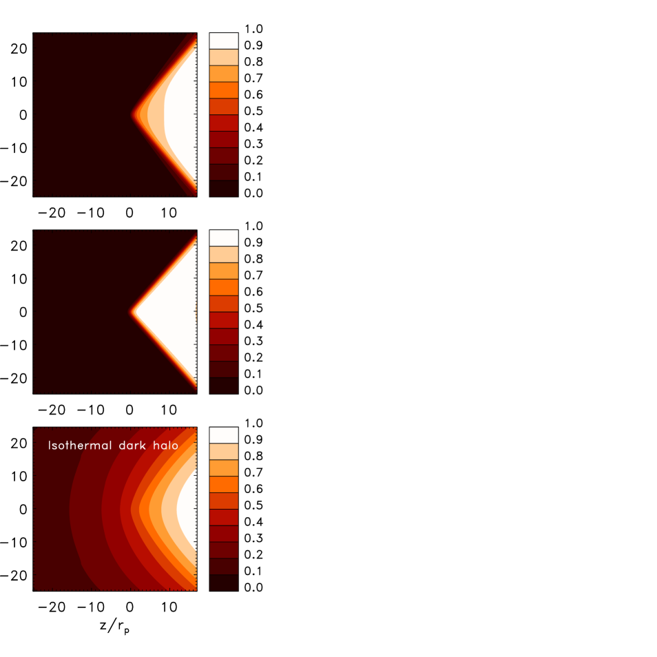
Figure 7: Normalized X-ray surface brightness maps for a ‘compact’ body moving at ${\mathcal{M}}=1.25$ in the deep-MOND non-axisymetric case for a line-of-sight along the $y$-axis (upper panel) and along the $x$-axis (middle panel), along with the X-ray map for an ‘extended’ pseudo-isothermal body in Newtonian gravity (bottom). The background field lays along the $x$-axis. The observer’s line of sight makes an angle $\pi/2$ with respect the velocity of the perturber.

In the Appendix A, we estimate the Bondi-Hoyle radius for a point mass in MOND. It is shown that the MOND Bondi-Hoyle radius is larger than in Newtonian gravity by a factor between $\mu_{0}^{-1}$ and $\mu_{0}^{-1}(1+L_{0})^{-1/2}$, depending on the angle between the velocity of the particle and the external field. To get a sense of values of $r_{BH}$ in typical cases, consider a galaxy of $5\times 10^{11}$ M_⊙ orbiting supersonically ${\mathcal{M}}\approx 1.5$ in a cluster of galaxies with a sound speed of intracluster gas of $\sim 1500$ km s^-1. The Bondi-Hoyle radius in this case is $r_{BH}\lesssim\mu_{0}^{-1}$ kpc. In a typical galactic cluster $\mu_{0}=0.3$–$1$ (see, e.g., fig. 7 in Sanders & McGaugh 2002), hence $r_{BH}\lesssim 1$–$3$ kpc, implying that, if the interaction with the intracluster gas is merely gravitational, the linear approximation is satisfactory for studying the gaseous wake even quite close to the galaxy. For extended perturbers with characteristic size much larger than $2r_{BH}$, the flow is essentially laminar at any location. In the remainder of the paper we will describe the perturbation on the gas using linear theory.

3 Formulation

3.1 Modelling the perturber

Our aim is to study the large-scale gravitational perturbation induced by a small perturber travelling through a much larger system. We obtain that, beyond a certain distance from the perturber, $|\mn@boldsymbol{\nabla}\Phi_{1}|\ll g_{\rm ext}$. In other words, the far-field wake is expected to be in the external field-dominated regime. In order to highlight the differences between genuine MOND and Newtonian gravity, we restrict our considerations to situations in which the potential is dominated by the external field everywhere, i.e., we will consider an extended perturber of mass $M$ and characteristic size $r_{p}$, where the internal acceleration $g_{\rm int}\approx GM_{p}/(\mu_{0}r_{p}^{2})\ll g_{\rm ext}$. The following density-potential pair, which corresponds to a “modified” Plummer model, is an exact solution of Eq. (4)

$$\rho_{p}(\mn@boldsymbol{r})=\frac{3Mr_{p}^{2}}{4\pi\sqrt{1+L_{0}}\left(x^{2}+y^{2}+\frac{z^{2}}{1+L_{0}}+r_{p}^{2}\right)^{5/2}},$$ (5)

$$\Phi_{p}(\mn@boldsymbol{r})=-\frac{1}{\mu_{0}}\frac{GM}{\sqrt{(1+L_{0})(x^{2}+y^{2})+z^{2}+\bar{r}_{p}^{2}}},$$ (6)

where $r_{p}$ and $\bar{r}_{p}\equiv(1+L_{0})^{1/2}r_{p}$ are the characteristic radii. Note that for $L_{0}=0$ and $\mu_{0}=1$ (Newtonian limit), it corresponds to the classical spherical Plummer model. Sometimes it is useful to express $\rho_{p}$ in terms of the central density of the object, $\rho_{c}$, as follows

$$\rho_{p}(\mn@boldsymbol{r})=\rho_{c}\left[1+\frac{x^{2}}{r_{p}^{2}}+\frac{y^{2}}{r_{p}^{2}}+\frac{z^{2}}{(1+L_{0})r_{p}^{2}}\right]^{-5/2},$$ (7)

where

$$\rho_{c}=\frac{3M}{4\pi(1+L_{0})^{1/2}r_{p}^{3}}.$$ (8)

The central density can be written in terms of the central density for the spherical Plummer model in classical Newtonian gravity, $\tilde{\rho}_{c}$, as $\rho_{c}=\tilde{\rho}_{c}/(1+L_{0})^{1/2}$.

The selection of a Plummer model was for analytical purposes. As long as the size of the system is much larger than the perturber, the structure of the wake and the drag force experienced by the perturber are not expected to be sensitive to the details of the potential close to the body.

In order to approach this problem analytically, we study the simplest case: an externally dominated perturber. In real life, there are some Galactic dwarf spheroidal galaxies that are known to be in this regime (e.g., Milgrom 1995; Sánchez-Salcedo & Hernandez 2007). It is likely that some subclusters and groups of galaxies, with low internal accelerations, embedded in a main massive galaxy cluster (such as the NGC 4911 group in the Coma Cluster) lie also in this regime (e.g., Sanders & McGaugh 2002).

In Eqs (5) and (6), the external field was taken along $z$ and, therefore, in the same direction as the incident flow (see Eq. 1). In this section we will focus on this axisymmetric case. The derivation of the equations when $\mn@boldsymbol{g}_{\rm ext}$ is perpendicular to $\mn@boldsymbol{v}_{\infty}$ is postponed up to §4.1.3. These two situations brackets a general case where the external field has an arbitrary angle with respect to the velocity of the flow at infinity.

3.2 Linear equations in an external dominated field

In the following, we give the linear derivation of the wake in a medium with unperturbed density $\rho_{0}$ and adiabatic sound speed $c_{\infty}$, ignoring gas self-gravity and any magnetic fields. As stated in Eq. (1), it is assumed that the gravitational perturber is seated at the origin of our coordinate system and the gas velocity far from the perturber is $\mn@boldsymbol{v}_{\infty}={\mathcal{M}}c_{\infty}\hat{z}$. In the axisymmetric case, $\mn@boldsymbol{v}_{\infty}$ and $\mn@boldsymbol{g}_{\rm ext}$ are parallel. We are interested in the steady-state density enhancement ${\mathcal{D}}(\mn@boldsymbol{r})=(\rho-\rho_{0})/\rho_{0}$ produced by the gravitational interaction with the perturber. The steady-state linearized basic dynamical equations for adiabatic perturbations $\rho=\rho_{0}+\rho^{\prime}$ and $\mn@boldsymbol{v}=\mn@boldsymbol{v}_{\infty}+\mn@boldsymbol{v}^{\prime}$ are:

$$\rho_{0}\mn@boldsymbol{\nabla}\mn@boldsymbol{v}^{\prime}+\mn@boldsymbol{v}_{\infty}\cdot\mn@boldsymbol{\nabla}\rho^{\prime}=0,$$ (9)

and

$$(\mn@boldsymbol{v}_{\infty}\cdot\mn@boldsymbol{\nabla})\mn@boldsymbol{v}^{\prime}=-\frac{c_{\infty}^{2}}{\rho_{0}}\mn@boldsymbol{\nabla}\rho^{\prime}-\mn@boldsymbol{\nabla}\Phi_{p}.$$ (10)

Our strategy is to eliminate $\mn@boldsymbol{v}^{\prime}$ everywhere. By substituting equation (9) in the divergence of equation (10), we obtain that ${\mathcal{D}}$ satisfies the differential equation

$$L{\mathcal{D}}=-\frac{1}{c_{\infty}^{2}}\nabla^{2}\Phi_{p},$$ (11)

where $L$ is the linear differential operator

$$L{\mathcal{D}}\equiv\frac{\partial^{2}{\mathcal{D}}}{\partial x^{2}}+\frac{\partial^{2}{\mathcal{D}}}{\partial y^{2}}+\left(1-{\mathcal{M}}^{2}\right)\frac{\partial^{2}{\mathcal{D}}}{\partial z^{2}}.$$ (12)

The operator $L$ arises frequently in fluid dynamics (e.g., Landau & Lifshitz 1959).

In Eqs (9)-(12) we have not specified the law of gravity. In MOND, the Laplacian of the potential in Eq. (11) can be expressed in terms of $\rho_{p}$ using the MOND field equation (4). The equation for ${\mathcal{D}}$ becomes

$$L{\mathcal{D}}=-\frac{4\pi G\rho_{p}}{\mu_{0}c_{\infty}^{2}}+\frac{L_{0}}{c_{\infty}^{2}}\frac{\partial^{2}\Phi_{p}}{\partial z^{2}}.$$ (13)

From now on, it will be convenient to use the following dimensionless variables: $\hat{x}=x/r_{p}$, $\hat{y}=y/r_{p}$ and $\hat{z}=z/(1+L_{0})^{1/2}r_{p}$. The hat symbol over a certain variable $\chi$ will be used to denote that $\chi$ is written with $\hat{x}$, $\hat{y}$ and $\hat{z}$ as the arguments, e.g., $\hat{D}(\hat{x},\hat{y},\hat{z})=D(x,y,z)$. The second-order derivative in Eq. (13) can be performed as soon as the potential is known. Evaluating the second-order derivative of the potential in Eq. (13) using the potential given in Eq. (6), and rearranging and grouping the terms, the solution $\hat{\mathcal{D}}$ can be expressed as a linear superposition of two contributions $\hat{\mathcal{D}}=\hat{\mathcal{D}}_{1}+\hat{\mathcal{D}}_{2}$. Each one satisfies the following differential equations:

$$\hat{L}{\hat{\mathcal{D}}}_{1}=-\left[1-T_{0}\right]\frac{4\pi G\rho_{c}r_{p}^{2}}{\mu_{0}c_{\infty}^{2}}\hat{g}_{1}(\hat{\mn@boldsymbol{r}}),$$ (14)

and

$$\hat{L}{\hat{\mathcal{D}}}_{2}=-T_{0}\frac{4\pi G\rho_{c}r_{p}^{2}}{\mu_{0}c_{\infty}^{2}}\hat{g}_{2}(\hat{\mn@boldsymbol{r}}),$$ (15)

with

$$\hat{g}_{1}(\hat{\mn@boldsymbol{r}})=\frac{1}{[1+\hat{r}^{2}]^{5/2}},$$ (16)

$$\hat{g}_{2}(\hat{\mn@boldsymbol{r}})=\frac{2\hat{z}^{2}-\hat{x}^{2}-\hat{y}^{2}}{[1+\hat{r}^{2}]^{5/2}},$$ (17)

where $\hat{r}^{2}=\hat{x}^{2}+\hat{y}^{2}+\hat{z}^{2}$,

$$T_{0}=\frac{L_{0}}{3(1+L_{0})},$$ (18)

and the operator $\hat{L}$ is

$$\hat{L}=\frac{\partial^{2}}{\partial\hat{x}^{2}}+\frac{\partial^{2}}{\partial\hat{y}^{2}}+\left(1-{\mathcal{M}}^{2}_{\rm eff}\right)\frac{\partial^{2}}{\partial\hat{z}^{2}},$$ (19)

with

$${\mathcal{M}}^{2}_{\rm eff}\equiv\frac{{\mathcal{M}}^{2}+L_{0}}{1+L_{0}}.$$ (20)

According to Eq. (18), $T_{0}$ varies from $0$ in the Newtonian regime ($L_{0}=0$) to $1/6$ in the deep MOND regime (i.e. $L_{0}=1$). From Eq. (20) it can be seen that ${\mathcal{M}}_{\rm eff}\geq{\mathcal{M}}$ in the subsonic case, ${\mathcal{M}}_{\rm eff}\leq{\mathcal{M}}$ in the supersonic case, and ${\mathcal{M}}_{\rm eff}={\mathcal{M}}=1$ at the transonic velocity.

We recall that the equation for $\hat{\mathcal{D}}$ in the Newtonian case is

$$\hat{L}\hat{\mathcal{D}}=-\frac{4\pi G\tilde{\rho}_{c}r_{p}^{2}}{c_{\infty}^{2}}g_{1}(\hat{\mn@boldsymbol{r}}),$$ (21)

which is naturally recovered from the above equations just by taking $\mu_{0}=1$ and $L_{0}=0$ (so that ${\mathcal{M}}_{\rm eff}={\mathcal{M}}$). The component $\hat{\mathcal{D}}_{1}$ obeys a differential equation similar to the Newtonian case and hence is identical to the wake induced by a perturber with mass density $\hat{\rho}_{1}=(1-T_{0})(1+L_{0})^{-1/2}\tilde{\rho}_{c}g_{1}(\hat{\mn@boldsymbol{r}})$ in conventional Newtonian gravity, once $G$ has been replaced by a larger effective value $G/\mu_{0}$. The profile $\hat{\rho}_{1}$ corresponds to the classical (spherical) Plummer model in the transformed coordinates ($\hat{x},\hat{y},\hat{z}$), multiplied by a form factor between $0.59$ (deep-MOND limit) and $1$ (Newtonian limit). In analogy to the Newtonian case (Eq. 21), a fictitious Newtonian perturber with a pseudo-density mass density distribution $\hat{\rho}_{2}=T_{0}\rho_{c}\hat{g}_{2}$ generates a component identical to $\hat{\mathcal{D}}_{2}$. We refer to $\hat{\rho}_{2}$ as pseudo-density because it may take negative values. Interestingly, the total mass associated with this distribution is

$$\hat{M}_{2}={\mathcal{PV}}\int_{-\infty}^{\infty}\int_{-\infty}^{\infty}\int_{-\infty}^{\infty}\hat{\rho}_{2}\;d\hat{x}d\hat{y}d\hat{z}=0.$$ (22)

Our natural choice was to adopt the Cauchy principal value of the integral, which we denote by the symbol ${\mathcal{PV}}$ (e.g., Mathews & Walker 1970). Note that $\hat{\rho}_{2}$ decays more slowly with radius than $\hat{\rho}_{1}$. Hence, the pseudo-density $\hat{\rho}_{2}$ becomes larger than $\hat{\rho}_{1}$ at large radii. The importance of the contribution of ${\mathcal{D}}_{2}$ to the wake and to the gravitational drag is difficult to forsee without a quantitative study.

3.3 Formal solution

The solution of Eqs (14) and (15) can be obtained using the retarded Green’s function, which may be derived following different paths (e.g., Just & Kegel 1990; Ostriker 1999). In particular, the Green function can be found after Fourier transforming and imposing causality when choosing the contour of integration in the complex plane for ${\mathcal{M}}_{\rm eff}>1$ (e.g., Just & Kegel 1990; Furlanetto & Loeb 2002). In the steady-state, the perturbed density fields $\hat{\mathcal{D}}_{1}$ and $\hat{\mathcal{D}}_{2}$ are

$$\hat{\mathcal{D}}_{1}=\frac{1-T_{0}}{(1+L_{0})^{1/2}\mu_{0}}\frac{G\tilde{\rho}_{c}r_{p}^{2}}{c_{\infty}^{2}}\hat{I}_{1},$$ (23)

$$\hat{\mathcal{D}}_{2}=\frac{T_{0}}{(1+L_{0})^{1/2}\mu_{0}}\frac{G\tilde{\rho}_{c}r_{p}^{2}}{c_{\infty}^{2}}\hat{I}_{2},$$ (24)

where

$$\hat{I}_{i}(\hat{\mn@boldsymbol{r}})=\int d^{3}\hat{\mn@boldsymbol{r}}^{\prime}\frac{\xi^{\prime}\hat{g}_{i}(\hat{\mn@boldsymbol{r}}^{\prime})}{[(\hat{z}-\hat{z}^{\prime})^{2}-\beta_{\rm eff}^{2}(\hat{R}^{2}+\hat{R}^{\prime 2}-2\hat{R}\hat{R}^{\prime}\cos\theta^{\prime})]^{1/2}},$$ (25)

for $i=1,2$, with $\beta^{2}_{\rm eff}\equiv{\mathcal{M}}_{\rm eff}^{2}-1$ and

$$\xi^{\prime}=\left\{\begin{array}[]{ll}2&\mbox{if ${\mathcal{M}}_{\rm eff}>1$, and}\\ &\mbox{$z-z^{\prime}+\beta_{\rm eff}[R^{2}+R^{\prime 2}-2RR^{\prime}\cos\theta^{\prime}]^{1/2}>0$;}\\ 1&\mbox{if ${\mathcal{M}}_{\rm eff}<1$;}\\ 0&\mbox{otherwise.}\end{array}\right.$$

4 Results

4.1 The density structure of the wake

4.1.1 The component ${\mathcal{D}}_{1}$ in the axisymmetric case

Figure 1 shows the integral $\hat{I}_{1}$, which is proportional to the perturbed density $\hat{D}_{1}$, in the $\hat{z}$–$\hat{R}$ plane, of a ${\mathcal{M}}_{\rm eff}=0.8,1.13,1.5$ body. In the deep MOND regime, they correspond to physical Mach numbers of $0.53$, $1.25$ and $1.9$, respectively. So far we are only interested in the ‘far-field’ perturbed density, hence we will not delve into details regarding the near-field (within a few core radius from the perturber). A subsonic perturber generates a density distribution with contours of constant density corresponding to similar ellipses with eccentricity ${\mathcal{M}}_{\rm eff}$. For supersonic motions, however, the region of perturbed density is confined within the rear Mach cone, dragged by its apex by the perturber. The surfaces of constant density within the wake correspond to hyperbolae in the $\hat{z}$–$\hat{R}$ plane, with eccentricity $e={\mathcal{M}}_{\rm eff}$. This is expected because, as we show in Section 3.2, the equation for $\hat{\mathcal{D}}_{1}$ has the same form as in the Newtonian case with ${\mathcal{M}}_{\rm eff}$, once the density distribution of the perturber is rescaled by a factor $(1-T_{0})(1+L_{0})^{-1/2}$, and $G$ is replaced by $G/\mu_{0}$. Using this analogy, we can take advantage of the analytical results of Ostriker (1999) to find the ’far-field’ perturbed density:

$${\mathcal{D}}_{1} \simeq \frac{1-T_{0}}{(1+L_{0})^{1/2}}\frac{\mu_{0}^{-1}\xi^{\prime\prime}G\hat{M}_{1}r_{p}^{2}/c_{\infty}^{2}}{\sqrt{\hat{z}^{2}-\beta_{\rm eff}^{2}\hat{R}^{2}}}$$ (26)

$$= (1-T_{0})\frac{\mu_{0}^{-1}\xi^{\prime\prime}GM/c_{\infty}^{2}}{\sqrt{z^{2}-\beta^{2}R^{2}}},$$ (27)

where $\xi^{\prime\prime}=2$ for supersonic perturbers and $1$ in the subsonic regime. In Eq. (27) we used that $\hat{M}_{1}=\tilde{\rho}_{c}\int\hat{g}_{1}d\hat{x}d\hat{y}d\hat{z}=M/r_{p}^{3}$. From the equation above, we see that the isodensity contours are $z^{2}+R^{2}(1-{\mathcal{M}}^{2})=$const, i.e. ellipses or hyperbolae with eccentricity $e={\mathcal{M}}$. In the Appendix B we reconsider the perturbation as a time-dependent rather than a steady state problem.

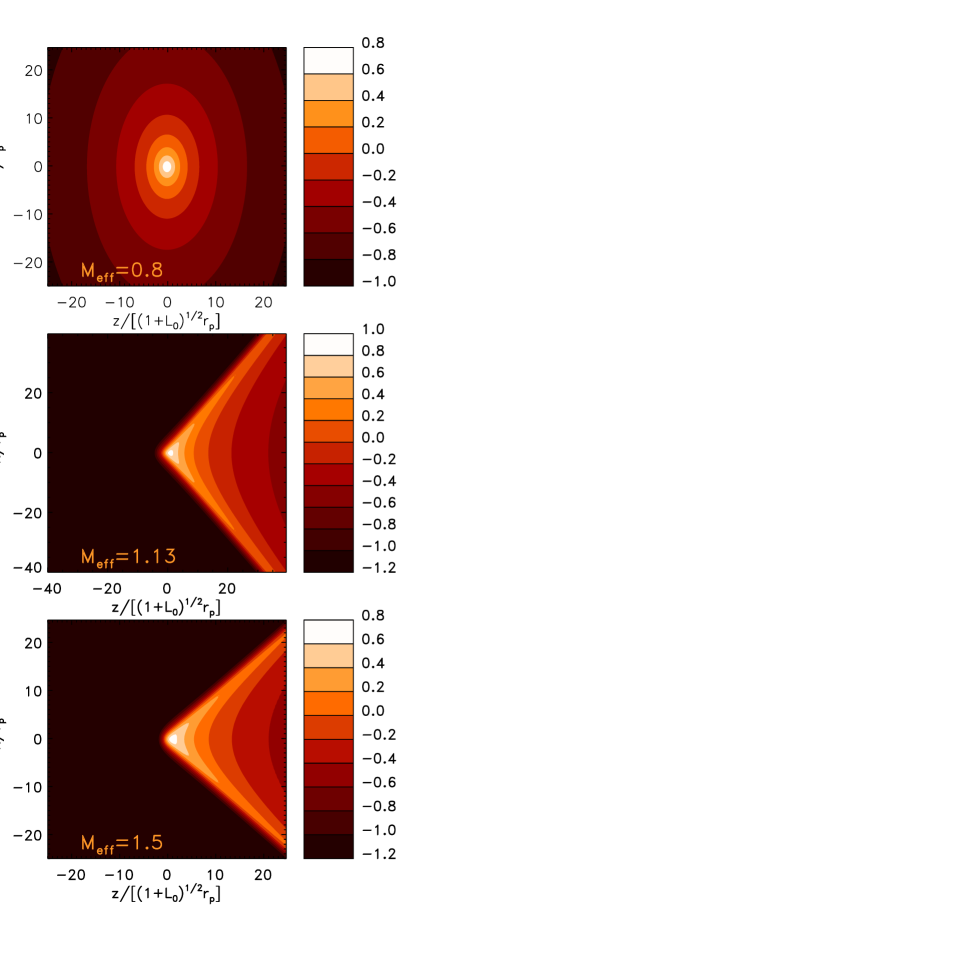
Figure 1: Distribution of the dimensionless integral $\hat{I}_{1}$, in logarithmic scale, for ${\mathcal{M}}_{\rm eff}=0.8,1.13$ and $1.5$ in the axisymmetric case. The box size for ${\mathcal{M}}_{\rm eff}=1.13$ is larger in order to have the same dynamical range in density.

4.1.2 The component ${\mathcal{D}}_{2}$ in the axisymmetric case

Figure 2 shows $\hat{I}_{2}$ for the same three effective Mach numbers as previously considered (${\mathcal{M}}_{\rm eff}=0.8$, $1.13$ and $1.5$). In the subsonic regime, $\hat{I}_{2}$, with a bipolar structure, is positive along the $z$ axis and negative in the perpendicular plane. For supersonic perturbers, an overdense bump at the head of the perturber is generated. Interestingly, $\hat{I}_{2}$ displays a drop in density along the surface of the Mach cone. This negative jump in the surface of the Mach cone is very remarkable at ${\mathcal{M}}_{\rm eff}=1.13$ and dilutes at larger effective Mach numbers. Our calculations show that at ${\mathcal{M}}_{\rm eff}=1.75$ there is no jump in the Mach cone surface. For perturbers with ${\mathcal{M}}_{\rm eff}>1.75$ the density jump in the Mach cone becomes positive. We see that, in general, $\hat{I}_{2}$ may take values comparable to $\hat{I}_{1}$. We note, however, that the real density $\hat{D}_{2}$ is related to $\hat{I}_{2}$ through a factor $T_{0}\leq 1/6$ (see Eq. 24).

Figure 3 contains the superposition $(1-T_{0})\hat{I}_{1}+T_{0}\hat{I}_{2}$, which is proportional to ${\mathcal{D}}$, in the deep MOND regime (i.e. $L_{0}=1$ and $T_{0}=1/6$). In the subsonic regime, the inclusion of the component ${\mathcal{D}}_{2}$ plays an important role. The resulting contours of isodensity can be fitted by ellipsoids defined by the equation $R^{2}+z^{2}/q^{2}=$const, where $q$ is the flattening parameter of the distribution in the physical $R$–$z$ plane. According to our discussion in the preceding section, for ${\mathcal{M}}_{\rm eff}=0.8$ and $L_{0}=1$ (i.e. ${\mathcal{M}}=0.53$), we know that the isodensity contours of ${\mathcal{D}}_{1}$ have $q=0.85$. The superposition of components ${\mathcal{D}}_{1}$ plus ${\mathcal{D}}_{2}$ generates a density distribution with $q=1.23$ (in the deep-MOND regime). In order to have an axis ratio of $q=0.85$, the body should be moving at ${\mathcal{M}}=0.85$. For ${\mathcal{M}}=0.2$, the flattening parameter is $0.98$ if only ${\mathcal{D}}_{1}$ is considered, and becomes $1.38$ when ${\mathcal{D}}_{2}$ is also taken into account. As a general conclusion, the wake for a subsonic body is more flattened along the direction of motion in MOND than in Newtonian dynamics.

In the supersonic deep-MOND case, the overdensity head is still visible when both components are added. The inclusion of ${\mathcal{D}}_{2}$, however, does not change significantly the structure of the wake within the Mach cone for ${\mathcal{M}}_{\rm eff}\leq 1.5$. At larger Mach number the contribution of ${\mathcal{D}}_{2}$ relative to ${\mathcal{D}}_{1}$ becomes less and less important. Since the structure of ${\mathcal{D}}_{1}$ is a scaled version of the wake generated in the Newtonian case, the difference between the structure of a wake generated by a small highly-supersonic perturber in MOND, would be likely too subtle to be distinguished from a perturber of fictitious mass $(1-T_{0})\mu_{0}^{-1}$ in Newtonian gravity. Differences only appear in the vicinity of the perturber.

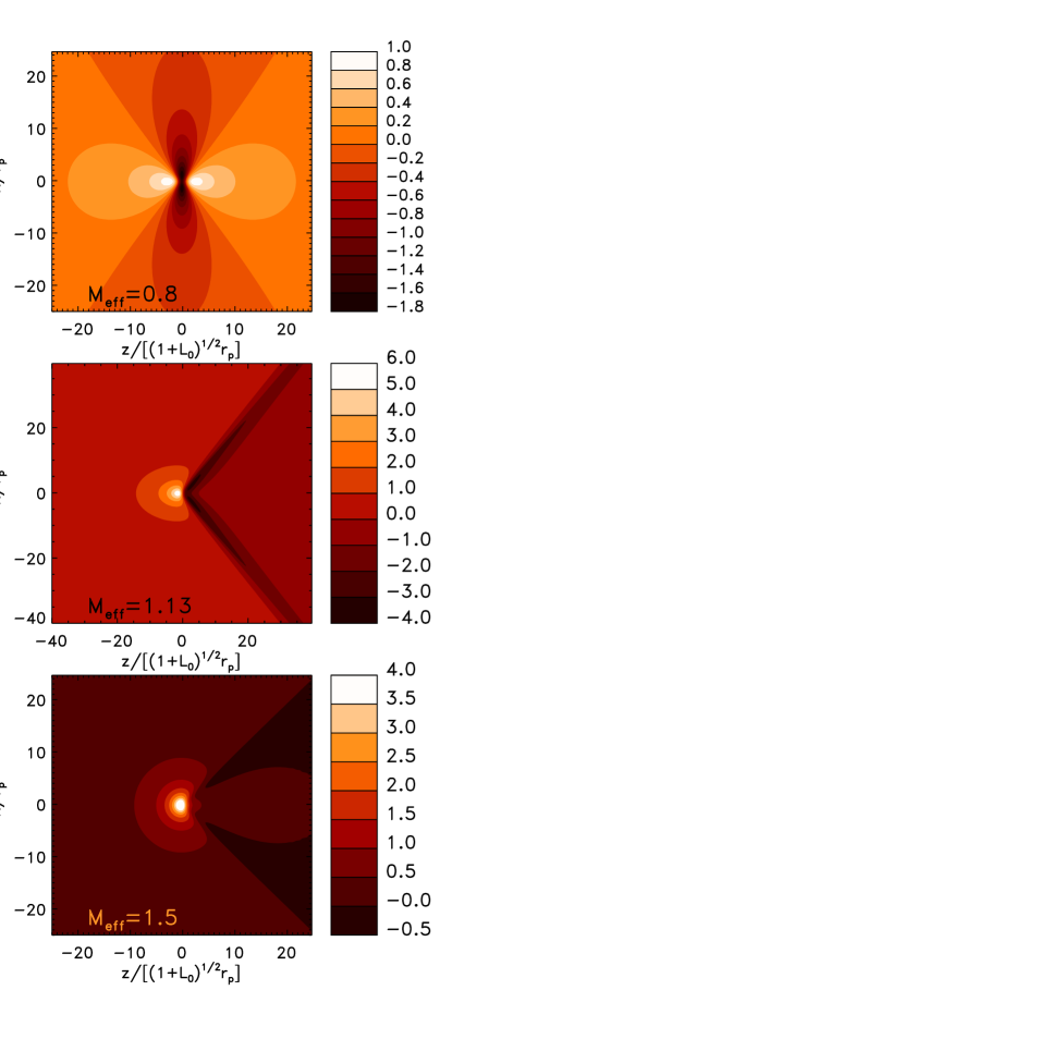
Figure 2: Profile of the dimensionless integral $\hat{I}_{2}$, in the axisymmetric case. The scale is linear scale. The effective Mach numbers are the same as in Fig. 1.

4.1.3 External field orthogonal to the velocity flow

Suppose now that the external field is along the $x$-axis. By denoting now $\hat{x}=x/r_{p}$, $\hat{y}=y/r_{p}$, $\hat{z}=z/r_{p}$, and by reasoning entirely analogous to that leading to Eqs (14)-(20), one finds that when the external field is perpendicular to the velocity flow, ${\mathcal{M}}_{\rm eff}$, $\hat{g}_{1}$ and $\hat{g}_{2}$ are given by

$${\mathcal{M}}_{\rm eff}={\mathcal{M}},$$ (28)

$$\hat{g}_{1}(\hat{\mn@boldsymbol{r}})=\left[1+\frac{\hat{x}^{2}}{1+L_{0}}+\hat{y}^{2}+\hat{z}^{2}\right]^{-5/2},$$ (29)

and

$$\hat{g}_{2}(\hat{\mn@boldsymbol{r}})=\left[\frac{2\hat{x}^{2}}{1+L_{0}}-\hat{y}^{2}-\hat{z}^{2}\right]\hat{g}_{1}.$$ (30)

In this case, the dependence on $L_{0}$ does not factorize so that one needs to calculate the integrals (25) for each pair $({\mathcal{M}}_{\rm eff},L_{0})$.

We found numerically that ${\mathcal{D}}_{1}$ is very axisymmetric around the $x$ axis; the effect of the gravitational dilation on ${\mathcal{D}}_{1}$ is small. For instance, when adopting $L_{0}=1$, the angular variations of ${\mathcal{D}}_{1}$ are less than $2\%$, $2\%$, $8\%$ and $13\%$ for ${\mathcal{M}}=0.4$, ${\mathcal{M}}=0.8$, ${\mathcal{M}}=1.25$ and ${\mathcal{M}}=1.8$, respectively. ${\mathcal{D}}_{1}$ is almost undistinguishable (differences of $\sim 5$ percent or less) from its counterpart in the axisymmetric case, and thus they are not shown. In particular, the opening angle of the Mach cone for supersonic perturbers in physical coordinates ($z,R$), is the same as in the axisymmetric case.

Unlike ${\mathcal{D}}_{1}$, ${\mathcal{D}}_{2}$ is expected to depart from axisymmetry about the $z$ axis. We will focus again on the deep-MOND limit ($L_{0}=1$). Figure 4 shows $\hat{I}_{2}$, which is proportional to ${\mathcal{D}}_{2}$, in three perpendicular planes: $y=0$, $x=0$ and $z=10r_{p}$, for ${\mathcal{M}}=0.53$ and ${\mathcal{M}}=1.25$. When the perturber moves subsonically, the structure of ${\mathcal{D}}_{2}$ in the $y=0$ plane looks pretty much like in the axisymmetric case after a rotation of $\pi/2$ (compare Fig. 2 and Fig. 4). In the $x=0$ plane, however, the density map is notoriously different. It clearly shows that the configuration $\hat{\mathcal{D}}_{2}$ has not an axial symmetry around the $z$ axis.

For subsonic perturbers, ${\mathcal{D}}_{2}$ may be able to change the flattening parameter of the wake. As an example, consider ${\mathcal{M}}=0.8$ and $L_{0}=1$. In this situation, ${\mathcal{D}}_{1}$ has isodensity contours with $q=0.6$. If the contribution of ${\mathcal{D}}_{2}$ is added, the composed wake exhibits $q=0.43$ in the $y=0$ plane, and $q=0.54$ in the $x=0$ plane (not shown).

For a supersonic perturber, the overdensity regions in ${\mathcal{D}}_{2}$ are not located any longer at the head of the body; regions at the front exhibit a decrease in density. Zones with density depletion, that is ${\mathcal{D}}_{2}<0$, can be found at both downstream and upstream. The maximum density enhancement in ${\mathcal{D}}_{2}$ appears smaller, by a factor $\sim 4$ at ${\mathcal{M}}=1.25$, than in the axisymmetric configuration. Figure 4 shows the complexity of the structure in the $(x,y)$ plane (lower panels). The isodensity contours in that plane turn up to be elongated along the $x$-axis.

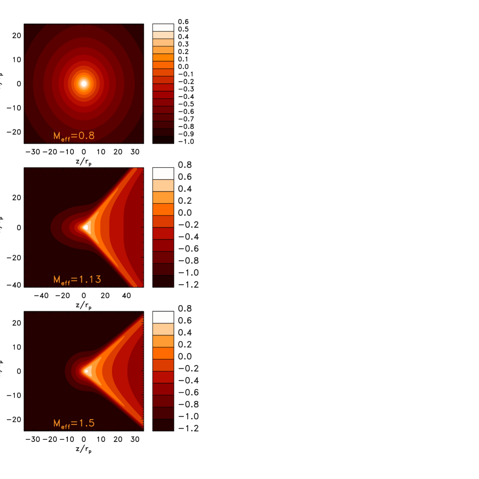
Figure 3: Density perturbation profiles, $\rho/\rho_{0}$, in units of $\mu_{0}^{-1}[G\tilde{\rho}_{c}r_{p}^{2}/\sqrt{2}c_{\infty}^{2}]$ in the axisymmetric case and with $L_{0}=1$. The scale is logarithmic.

4.2 The gravitational drag on the body

Once the structure of the wake ${\mathcal{D}}$ is constructed, it is straightforward to evaluate the drag force exerted on the perturber by its wake. By symmetry, the only non-vanishing component lies along the $z$ axis. In particular, the drag force in the axisymmetric case is

$$F_{DF}=2\pi\frac{GM\rho_{0}}{\mu_{0}}\int\int dzdRR\frac{{\mathcal{D}}z}{((1+L_{0})R^{2}+z^{2}+\bar{r}_{p}^{2})^{3/2}}.$$ (31)

If $F_{DF,1}$ and $F_{DF,2}$ denote the contribution to the drag force by components ${\mathcal{D}}_{1}$ and ${\mathcal{D}}_{2}$, respectively, we have:

$$F_{DF}=F_{DF,1}+F_{DF,2},$$ (32)

$$F_{DF,1}=\frac{3}{2}\frac{1-T_{0}}{\mu_{0}^{2}(1+L_{0})}\frac{G^{2}M^{2}\rho_{0}}{c_{\infty}^{2}}{\mathcal{F}}_{1},$$ (33)

$$F_{DF,2}=\frac{3}{2}\frac{T_{0}}{\mu_{0}^{2}(1+L_{0})}\frac{G^{2}M^{2}\rho_{0}}{c_{\infty}^{2}}{\mathcal{F}}_{2},$$ (34)

where

$${\mathcal{F}}_{i}=\int\int d\hat{z}d\hat{R}\frac{\hat{I}_{i}\hat{R}\hat{z}}{(1+\hat{R}^{2}+\hat{z}^{2})^{3/2}}.$$ (35)

We first estimate the relative contribution of $F_{DF,2}$ as compared to $F_{DF,1}$. For supersonic perturbers, ${\mathcal{F}}_{2}$ and ${\mathcal{F}}_{1}$ were calculated by carrying out the integration in Eq. (35) over all our box domain. Hence, the $\hat{z}$-integral has upper/lower limits $\hat{z}=\pm 25$ and the $\hat{R}$-integral has limits $\hat{R}=0,25$. This implies that our steady-state wakes have an extent along $z$ of $z_{\rm max}\sim 25r_{p}$ to $35r_{p}$, depending on $L_{0}$, and a Coulomb logarithm $\ln\Lambda\sim\ln z_{\rm max}/2r_{p}\sim 3$ (Sánchez-Salcedo & Brandenburg 1999).

Figure 4: Distribution of the dimensionless integral $\hat{I}_{2}$ at cut-off planes $y=0$ (upper), $x=0$ (middle) and $z=10r_{p}$ (lower) for ${\mathcal{M}}=0.53$ (left column) and ${\mathcal{M}}=1.25$ (right column), in linear scale. The velocity of the perturber is along the $z$-axis, whereas the external gravitational acceleration is along the $x$-axis and $L_{0}=1$.

For a purely steady-state density perturbation, the forward-backward symmetry in the subsonic case argues that zero net force acts on the perturber. However, Ostriker (1999) noticed that this conclusion is misleading because, although complete ellipsoids exert no net force on the perturber, there are always cut-off ones within the sonic sphere that exert a gravitational drag. Thus, we estimate the gravitational drag on a subsonic perturber by integrating Eq. (35) over the largest sonic sphere contained in our computational domain.

The ratio ${\mathcal{F}}_{2}/{\mathcal{F}}_{1}$ depends on the angle between $\mn@boldsymbol{v}_{\infty}$ and $\mn@boldsymbol{g}_{\rm ext}$. For illustration, Fig. 5 shows its behaviour as a function of ${\mathcal{M}}_{\rm eff}$ for supersonic bodies moving along the external gravitational field. In such a case, ${\mathcal{F}}_{2}$ is positive at large Mach numbers, implying that it contributes to drag the body. It becomes zero at ${\mathcal{M}}_{\rm eff}\simeq 1.75$ and negative for lower values. The relative contribution of ${\mathcal{D}}_{2}$ becomes more important when approaching the transonic motion. At large Mach numbers, the ratio ${\mathcal{F}}_{2}/{\mathcal{F}}_{1}$ increases monotonically but very slowly.

In order to visualize the importance of including $F_{DF,2}$, Figure 6 shows the total drag force exerted on the perturber as a function of ${\mathcal{M}}$, together with $F_{DF,1}$, in the deep-MOND limit ($L_{0}=1$, $T_{0}=1/6$). As anticipated, the sign of $F_{DF,2}$ depends on the angle between $\mn@boldsymbol{v}_{\infty}$ and $\mn@boldsymbol{g}_{\rm ext}$. In contrast to the axisymmetric case, when $\mn@boldsymbol{v}_{\infty}$ and $\mn@boldsymbol{g}_{\rm ext}$ are perpendicular, $F_{DF,2}$ is positive for transonic Mach numbers and becomes negative (reduces friction) at high Mach numbers. The contribution to the drag by the component ${\mathcal{D}}_{2}$ is more important in the axisymmetric case but it is only noticeable ($>20\%$) at $1<{\mathcal{M}}<1.5$. Our numerical calculations show that $F_{DF,1}$ scales with the size of the box domain as $\propto\ln z_{\rm max}$, whereas $F_{DF,2}$ increases somewhat slower with $z_{\rm max}$. Therefore, the relative importance of $F_{DF,2}$ is expected to be less for larger $z_{\rm max}$.

Now, we wish to compare the drag force in deep MOND ($L_{0}=1$) and in Newtonian gravity ($L_{0}=0$). Figure 6 also shows the Newtonian drag force experienced by a body of mass $M$, travelling at Mach number ${\mathcal{M}}$ when the wake has the same extent as in the MOND case, i.e. $z_{\rm max}=25\sqrt{2}r_{p}$. The drag force in MOND is a factor $\alpha\mu_{0}^{-2}$ larger than in Newton, where $\alpha$ is a form factor that depends on the Mach number and on the angle between $\mn@boldsymbol{v}_{\infty}$ and $\mn@boldsymbol{g}_{\rm ext}$. In the axisymmetric case, $\alpha\simeq 0.6$ at low Mach numbers (${\mathcal{M}}\lesssim 0.5$), and becomes $\alpha\simeq 0.5$ at $0.5<{\mathcal{M}}\lesssim 1.0$. For supersonic Mach numbers, $\alpha\simeq 0.4$ at $1<{\mathcal{M}}\lesssim 1.5$ and increases monotonically with Mach number up to $\simeq 0.8$ at high Mach numbers. The explanation for $\alpha=0.8$ at high Mach numbers is covered in detail in the Appendix C. When the direction of motion is perpendicular to the external field, $\alpha$ is very similar to its value in the axisymmetric case at ${\mathcal{M}}<1$. At supersonic velocities, $\alpha\simeq 0.6$ at $1<{\mathcal{M}}\lesssim 1.5$, and falls monotonically down to $0.5$ at high Mach numbers. Hence, the drag force may vary with the angle between $\mn@boldsymbol{v}_{\infty}$ and $\mn@boldsymbol{g}_{\rm ext}$ by as much as $50$ percent.

5 Some implications

5.1 Wakes by galaxies and falling groups in clusters

In this section, we discuss the implications of X-ray observations of the morphology of wakes in clusters of galaxies for modified gravities. As in Furlanetto & Loeb (2002), let us assume that the galaxy or group of galaxies moves supersonically through a constant density cluster core surrounded by a isothermal envelope:

$$\rho_{IC}(r)=\left\{\begin{array}[]{ll}\rho_{0}&\mbox{if $r\leq r_{c}$};\\ 2\rho_{0}/[1+(r/r_{c})^{2}]&\mbox{if $r\geq r_{c}$}.\end{array}\right.$$

where $\rho_{0}$ is the density in the core and $r_{c}$ is the core radius. The emitted surface brightness $S=\int(\epsilon_{ff}/4\pi)dl$, where $\epsilon_{ff}$ is the bremsstrahlung free-free volume emissivity, will be enhanced in the wake by:

$$\frac{\delta S}{S}\sim\chi\frac{\delta\Sigma}{\Sigma},$$ (36)

where $\Sigma$ is the column density, and $\chi\approx 4$ if the gas is isothermal, or $\approx 5$ if it varies adiabatically (Furlanetto & Loeb 2002). Maps of X-ray for a ${\mathcal{M}}=1.25$ body with $\mn@boldsymbol{v}_{\infty}$ perpendicular to the external gravitational field are shown in Fig. 7. The structure of the emission in the wake is very similar to that formed by a “compact” gravitational perturber under Newton gravity. The projected X-ray emission along line-of-sights perpendicular to the direction of motion is roughly independent of the location in the wake, except near the edges of the cone, and is given by

$$\frac{\delta S}{S}\simeq\frac{2\pi\chi}{(2+\pi)}\frac{GM}{\mu_{0}\beta c_{\infty}^{2}r_{c}}.$$ (37)

As a consequence, in searching for the wake, one may expect an abrupt jump in surface brightness at the edge of its cone.

We derived the gravitational wake induced by an extended body with a Plummer profile having a fast density decay at large radii ($\rho\propto r^{-5}$) in an attempt to model the baryonic mass of a certain bound object. Wakes in the cold dark matter (CDM) scenario are expected to be different than in purely baryonic MOND because the dark matter component in the halo of galaxies decays as $r^{-2}$, much more slowly than the baryonic mass density ($\leq r^{-3}$). To illustrate this, Figure 7 also shows the X-ray emission generated by a pseudo-isothermal perturber with core radius $r_{p}$ in the Newtonian case. We see that the X-ray emission in the standard CDM scenario is more cuspy. A MOND wake can be distinguished from a CDM wake by detecting a sharp X-ray enhancement along the Mach cone. Furlanetto & Loeb (2002) made a detailed analysis of the wake morphology in CDM models for collisionless and fully collisional (fluid) dark matter (FDM) in the supersonic case. They found that, because in the collisional case the dark halo is truncated by ram pressure stripping, the X-ray emission of the wake is rather flat, similar to that we find in MOND. Due to the quantitative similarity between the wake in MOND and in FDM, many of the observational suggestions raised by Furlanetto & Loeb to distinguish between FDM and CDM can be used to distinguish between dark matter or MOND. We can repeat the reasoning of Furlanetto & Loeb (2002) and argue that the observations of the wake of the elliptical galaxy NGC 1404 in the core of the Fornax group marginally support CDM against MOND, but the evidence is very weak. In the last decade, this type of observations has improved considerably (e.g., Drake et al. 2000; Neumann et al. 2001; Machacek et al. 2005, 2007; Sun et al. 2006). Still, it is difficult to draw some firm conclusions because of the difficulty to isolate the structure of the gravitational wake from the hydrodynamical wake, that is the mass in the wake stripped from the own galaxy by ram pressure. We must warn that MOND and FDM predict the same structure of the gravitational wake past a galaxy but, in many other astrophysical aspects, they must give different predictions since they are not equivalent.

In principle, observations of the tails of subclusters of galaxies are a potential route to distinguish betweeen collisionless CDM and MOND. However, it is a well established issue that MOND still requires dark matter at cluster scales (e.g., The & White 1988; Sanders 1999). The inclusion of an isothermal dark matter component in MOND erases somewhat the abovementioned differences between the MOND wake and the CDM wake. The observed displacement between the X-ray peaks and the associated mass distribution, as derived from lensing data in the Bullet Cluster, basically rules out FDM (Markevitch et al. 2004) but not necessarily MOND (Angus et al. 2007).

Figure 5: Ratio between ${\mathcal{F}}_{2}$ and ${\mathcal{F}}_{1}$, as defined in Eq. (35), versus the effective Mach number, for the axisymmetric case. At ${\mathcal{M}}_{\rm eff}<1$, the ratio depends on the adopted value for $L_{0}$ and hence is not shown.

Figure 6: DF force in a gaseous medium as a function of the Mach number when $\mn@boldsymbol{v}_{\infty}$ and $\mn@boldsymbol{g}_{\rm ext}$ are parallel (top) and orthogonal (bottom). The open diamonds correspond to the drag by the component ${\mathcal{D}}_{1}$ in the deep-MOND limit and the asterisks correspond to the total drag. The dashed line and the triangles show the drag in Newtonian gravity. To help comparison, the total drag in the axisymmetric case and the Newtonian drag have been also plotted in the lower panel (dotted line and dashed line, respectively).

5.2 DF timescale in a spherical system

In §4.2 we derived the DF force experienced by a body of mass $M$ travelling on a rectilinear orbit through a homogeneous fluid medium in deep-MOND and found that:

$$F_{DF}=-\frac{\alpha}{\mu_{0}^{2}}\frac{4\pi G^{2}M^{2}\rho_{0}}{v_{\infty}^{2}}\ln\Lambda,$$ (38)

where $\alpha$ depends on the Mach number and on the angle that makes the velocity of the perturber and the direction of the external field. How does it compare with the DF force in a collisionless medium? The formula for the collisionless MOND DF force was derived by Ciotti & Binney (2004). They show that it is similar to the Newtonian case but replacing $G\rightarrow Ga_{0}/g_{\rm ext}$ plus an extra factor of $\sqrt{2}$:

$$F_{DF,{\rm no-col}}=-\frac{1}{\sqrt{2}\mu_{0}^{2}}\frac{4\pi G^{2}M^{2}\rho_{0}}{v_{\infty}^{2}}H\ln\Lambda,$$ (39)

where

$$H={\rm erf}\left(\frac{v_{\infty}}{\sqrt{2}\sigma}\right)-\sqrt{\frac{2}{\pi}}\frac{v_{\infty}}{\sigma}\exp\left(-\frac{v_{\infty}^{2}}{2\sigma^{2}}\right),$$ (40)

with $\sigma$ the velocity dispersion of the Maxwellian distribution of velocities of background particles (e.g., Binney & Tremaine 1987; Sánchez-Salcedo et al. 2006). By comparing Eqs (38) and (39), we can generalize the conclusion of Ostriker (1999) but for MOND: since the functional form of the gaseous DF drag is much more sharply peaked near ${\mathcal{M}}=1$, the drag force near ${\mathcal{M}}=1$ is larger in a gaseous medium than in a collisionless medium with the same density and $\sigma=c_{\infty}$. At ${\mathcal{M}}\approx 1$, using $\alpha\approx 0.5$ (see §4.2) there is factor of $\sim 3$ difference in the MOND force between the two cases. For ${\mathcal{M}}<1$, the drag force is generally larger in a collisionless medium than in a gaseous medium, because pressure forces in a gaseous medium create a much more symmetric density perturbation in the background.

For many problems of astrophysical interest, it is convenient to have the DF inspiraling timescale for a body that is initially on a circular orbit. For circular orbits, the above formula is correct as long as the maximum impact parameter in the Coulomb logarithm is taken as $\sim 2R_{p}$, where $R_{p}$ is the instantaneous orbital radius of the perturber (Sánchez-Salcedo & Brandenburg 2001; Kim & Kim 2007). Consider a massive body embedded in the gaseous outer spherical envelope of a galaxy of mass $M_{G}$, with circular speed $v_{c}=(GM_{G}a_{0})^{1/4}$. Suppose that the gas is isothermal and in hydrostatic equilibrium in the gravitational potential of the parent galaxy. In a typical galaxy, the outer parts are expected to be in the deep-MOND regime, hence $g_{\rm ext}=\sqrt{GM_{G}a_{0}}/r$ and $\mu_{0}=(GM_{G}/a_{0})^{1/2}r^{-1}$. For the sake of clarity, let us assume that the gas has the virial temperature: $c_{\infty}\simeq v_{c}/\sqrt{2}$. Imposing hydrostatic equilibrium, the unperturbed gas in the envelope will pursue the following profile

$$\rho_{g}=\rho_{s}\left(\frac{r}{r_{s}}\right)^{-2},$$ (41)

where $\rho_{s}$ is the gas density at the radius of reference $r_{s}$. By substituting the values for $\mu_{0}$ and $\rho_{g}$ into Eq. (38), and equating the rate of decrease of angular momentum $d(Mv_{c}r)/dt$ to the torque $rF_{DF}$, we find the deep-MOND evolution of the orbital decay of a massive perturber’s near-circular orbit in a gaseous isothermal spherical distribution

$$\frac{r}{r_{\rm init}}=\exp\left(-\frac{t-t_{\rm init}}{\tau_{M}}\right),$$ (42)

where $r_{\rm init}$ is the orbital radius at $t=t_{\rm init}$ and

$$\tau_{M}=\frac{\mu_{s}^{2}}{\alpha}\frac{v_{c}^{3}}{4\pi G^{2}M}\frac{1}{\rho_{s}\ln\Lambda},$$ (43)

with $\mu_{s}=\mu_{0}(r_{s})$.

Consider now its equivalent Newtonian system (ENS) that is, the Newtonian system (dark matter plus gas) in which the baryonic gas has exactly the same density distribution as in the MOND system. The density distribution of dark matter in the ENS is:

$$\rho_{dm}=\frac{v_{c}^{2}}{4\pi Gr^{2}}.$$ (44)

In the ENS, the dark matter component added to have the same “dynamics” also contributes to the DF experienced by the body. The frictional force in the ENS is

$$F_{DF}=-\frac{4\pi G^{2}M^{2}(\rho_{g}+0.428\rho_{dm})}{v_{c}^{2}}\ln\Lambda.$$ (45)

The factor $0.428$ arises because the dark matter has been considered collisionless (see, e.g., eq. [7-25] of Binney & Tremaine 1987). Equating again angular momentum loss with the torque, we find $\tau_{ENS}$, the time that the body takes to reduce its distance a factor $e$ in the ENS:

$$\tau_{ENS}=\frac{0.43}{1+0.428{\mathcal{R}}_{g}}\left(\frac{r_{\rm init}^{2}}{r_{s}^{2}}\right)\frac{v_{c}^{3}}{4\pi G^{2}M}\frac{1}{\rho_{s}\ln\Lambda},$$ (46)

where ${\mathcal{R}}_{g}\equiv\rho_{dm}/\rho_{g}=$const. The ratio between the DF timescale in MOND and in ENS is:

$$\frac{\tau_{M}}{\tau_{ENS}}=4.6(1+0.428{\mathcal{R}}_{g})\mu_{\rm init}^{2}.$$ (47)

Here $\mu_{\rm init}\equiv\mu_{0}(r_{\rm init})$ and we used that $\alpha\simeq 0.5$ for ${\mathcal{M}}=1.4$ (see §4.2). In terms of ${\mathcal{R}}_{t,{\rm init}}$ defined as the ratio between the mass in dark matter and the baryonic mass (stars plus gas) inside $r_{\rm init}$, we have

$$\frac{\tau_{M}}{\tau_{ENS}}=4.6(1+0.428{\mathcal{R}}_{g})\frac{1}{[1+{\mathcal{R}}_{t,{\rm init}}]^{2}}.$$ (48)

In dwarf protogalaxies, before the gas is turned into stars, ${\mathcal{R}}_{g}\simeq{\mathcal{R}}_{t}$, and for typical values of dark matter contents in these systems (${\mathcal{R}}_{t}\simeq 20$), the gaseous DF timescale in MOND is $10$ times shorter than in the ENS. Condensed objects that form early (e.g., globular clusters) could spiral into the centre of their host galaxy more rapidly than would be predicted in the standard CDM haloes.

6 Summary

After a discussion about the Bondi-Hoyle problem, we have calculated the gravitational density wake of a perturber moving through a uniform gaseous medium in MOND. A hydrodynamical treatment provides useful insight into the problem of DF. In order to describe the response of the far-field medium to a small perturber, we focused on the case when the perturbation is dominated by a constant external field. The analytical knowledge of the wake structure in this simple case is useful to interpret fully non-linear simulations of the MOND dynamics of realistic systems. The structure of the wake depends on the angle between the velocity vector and the external gravitational field. We have considered two cases: the velocity of the perturber being either parallel or orthogonal to the external field. For an intermediate case, the structure of the wake will lay somewhere between the extremes described here. The density wake is decomposed into two linear contributions. The morphology of the dominant contribution is a scaled version of the Newtonian wake, being the MOND perturbed density a factor $\mu_{0}^{-2}$ larger than in Newtonian gravity. The second contribution to the wake depends greatly on the angle which the direction of motion makes with the external field.

The MOND DF force on the perturber induced by its own wake, as a function of the Mach number has been also derived and compared with the drag force in the Newtonian case. It is important to know the dependence of the drag force strength on Mach number to study the circularization of orbits. Our results confirm earlier analyses suggesting that the DF force is higher in MOND than in Newtonian gravity. The DF drag is larger when the motion of the perturber is along the external field, especially at Mach numbers between $1$–$1.5$. In the context of the sinking satellite problem, the recent claim that the existence of an extended globular cluster population in Fornax is problematic for MOND gains strength (Sánchez-Salcedo et al. 2006; Nipoti et al. 2008). We find that MOND predicts an even faster orbital decay, especially when the satellite arrives to the halo of a galaxy before the gas has turned into stars.

In MOND we show that a supersonic perturber generates a wake in the gas with a well-defined Mach cone in which the the surface density increases substantially in a narrow region and then flattens. Because CDM haloes extend to larger radii than the baryonic mass, the wakes in the two models have significant morphological differences.

Inherent to the Chandrasekhar treatment of DF is the assumption that the perturber interacts with unbound particles. In MOND, this requirement immediately demands the inclusion of the external field. Once the background gravitational field is included, two-body orbits of distant particles are unbound, the interaction of the perturber with the medium is quasi-Newtonian, and the effects of distant encounters can be simply added. This topic is closely related to studies of relaxation processes in self-gravitating media. In a forthcoming paper we will present a standard derivation of the DF drag in collisionless systems in MOND.

Appendix A The Bondi-Hoyle radius in MOND

For a point-like particle, the linear MOND field equation (Eq. 4) is readily solved (Milgrom 1986):

$$\Phi_{1}(\mn@boldsymbol{r})=-\frac{1}{\mu_{0}}\frac{GM}{\sqrt{(1+L_{0})(x^{2}+y^{2})+z^{2}}},$$ (49)

where we have supposed that the external field is along the $z$-axis. We are now in a position to derive the Bondi-Hoyle radius $r_{BH,1}$ for the potential $\Phi_{1}$. We know, however, that $\Phi_{1}$ is not a good approximation in the vicinity of the particle. Nevertheless, since $|\Phi_{1}|$ overestimates the depth of the potential once we approach the perturber (i.e. $|\Phi_{1}|\geq|\Phi_{\rm exact}|$, where $\Phi_{\rm exact}$ is the exact potential for a point mass), the Bondi-Hoyle radius derived using the potential $\Phi_{1}$ provides an upper limit to the exact Bondi-Hoyle radius.

In the rest frame of the perturber, consider a streamline that begins at $x,y,z$ coordinates $(x,y,-\infty)$. A straight streamline is susceptible to bending and shocking if the velocity of the gas on that streamline (adding the thermal velocity) is larger than the maximum value of the escape velocity along that streamline:

$$\frac{2}{\mu_{0}(1+L_{0})^{1/2}}\frac{GM}{\sqrt{x^{2}+y^{2}}}>v_{\infty}^{2}+c_{\infty}^{2},$$ (50)

where we have assumed that $\mn@boldsymbol{v}_{\infty}$ and $\mn@boldsymbol{g}_{\rm ext}$ lie both along the $z$-axis. According to the above equation, all the streamlines that start with impact parameter $b$ such as:

$$b<\frac{2}{\mu_{0}(1+L_{0})^{1/2}}\frac{GM}{c_{\infty}^{2}(1+{\mathcal{M}}^{2})}$$ (51)

bend significantly and go through shocks. In analogy with the Newtonian case, the MONDian Bondi-Hoyle radius is:

$$r_{BH,1}=\frac{1}{\mu_{0}(1+L_{0})^{1/2}}\frac{GM}{c_{\infty}^{2}(1+{\mathcal{M}}^{2})}.$$ (52)

If $\mn@boldsymbol{g}_{\rm ext}$ lies along the $x$-axis (so that $\mn@boldsymbol{g}_{\rm ext}$ and $\mn@boldsymbol{v}_{\infty}$ are perpendicular), the condition for blending is:

$$\frac{2}{\mu_{0}}\frac{GM}{\sqrt{x^{2}+(1+L_{0})y^{2}}}>v_{\infty}^{2}+c_{\infty}^{2}.$$ (53)

The streamlines subject to terminate in a shock are

$$\left(x^{2}+(1+L_{0})y^{2}\right)^{1/2}<\frac{2}{\mu_{0}}\frac{GM}{c_{\infty}^{2}(1+{\mathcal{M}}^{2})}.$$ (54)

We see that, due to the dilation along the axis of the background field, the curvature of streamlines with the same impact parameter depends on their azimuthal angle in the $(x,y)$ plane. Nevertheless, there is a guarantee that the response of the gas will be linear at any radius beyond $2r_{BH,1}$ where

$$r_{BH,1}=\frac{1}{\mu_{0}}\frac{GM}{c_{\infty}^{2}(1+{\mathcal{M}}^{2})}.$$ (55)

Appendix B The component ${\mathcal{D}}_{1}$ in the axisymmetric case for a time-dependent perturbation

We may be interested in the temporal evolution of the wake when the perturber is placed at $t=0$. The Newtonian case was studied by Ostriker (1999) who found that the induced wake density for this finite-time perturbation has the following analytic form

$${\mathcal{D}}_{N}(t)=\frac{\xi GM/c_{\infty}^{2}}{\sqrt{z^{2}-\beta^{2}R^{2}}},$$ (56)

where $\beta^{2}={\mathcal{M}}^{2}-1$ and

$$\xi=\left\{\begin{array}[]{ll}2&\mbox{if ${\mathcal{M}}>1$, $R^{2}+(z-v_{\infty}t)^{2}>(c_{\infty}t)^{2}$},\\ &\mbox{$z/R>\beta$, and $z<\beta c_{\infty}t/{\mathcal{M}}$};\\ 1&\mbox{if $R^{2}+(z-v_{\infty}t)^{2}<(c_{\infty}t)^{2}$};\\ 0&\mbox{otherwise.}\end{array}\right.$$

We can take advantage of this Newtonian result to get ${\mathcal{D}}_{1}(t)$ in MOND, at distances larger than a few $r_{p}$, as:

$${\mathcal{D}}_{1}(t) \simeq \frac{1-T_{0}}{(1+L_{0})^{1/2}}\frac{\mu_{0}^{-1}\xi G\hat{M}_{1}r_{p}^{2}/c_{\infty}^{2}}{\sqrt{\hat{z}^{2}-\beta_{\rm eff}^{2}\hat{R}^{2}}}$$ (57)

$$= (1-T_{0})\frac{\mu_{0}^{-1}\xi GM/c_{\infty}^{2}}{\sqrt{z^{2}-\beta^{2}R^{2}}}.$$

Here we used again that $\hat{M}_{1}=M/r_{p}^{3}$.

Appendix C The drag force in MOND and Newton at high Mach numbers

According to Eq. (33), the drag force experienced by a Plummer body in Newtonian gravity is:

$$F_{DF,N}=\frac{3}{2}\frac{G^{2}M^{2}\rho_{0}}{c_{\infty}^{2}}{\mathcal{F}}_{1}.$$ (58)

Let us compare $F_{DF,N}$ with $F_{DF,1}$ at ${\mathcal{M}}\gg 1$ in the axisymmetric case. Note that at those Mach numbers $F_{DF,2}$ can be ignored. Combining Eqs (33) and (58), the drag force component $F_{DF,1}({\mathcal{M}},z_{\rm max})$ exerted on a body moving at ${\mathcal{M}}$ by a wake with extent $z_{\rm max}$ can be recast:

$$F_{DF,1}=\frac{1-T_{0}}{\mu_{0}^{2}(1+L_{0})}F_{DF,N}\left({\mathcal{M}}_{\rm eff},\hat{z}_{\rm max}\right).$$ (59)

In the limit ${\mathcal{M}}\gg 1$ and in the steady state, see e.g., Ostriker (1999),

$$F_{DF,N}\propto\frac{1}{v_{\infty}^{2}}\ln\left(\frac{z_{\rm max}}{r_{\rm min}}\right).$$ (60)

Therefore, for $z_{\rm max}\gg r_{\rm min}$, we have $F_{DF,N}\propto v_{\infty}^{-2}$ and

$$F_{DF,N}({\mathcal{M}}_{\rm eff})\simeq\left(\frac{{\mathcal{M}}}{{\mathcal{M}}_{\rm eff}}\right)^{2}F_{DF,N}({\mathcal{M}})$$

$$\simeq(1+L_{0})F_{DF,N}({\mathcal{M}}).$$ (61)

Substituting into Eq. (59), we find that the drag force exerted by ${\mathcal{D}}_{1}$ in the supersonic axisymmetric MOND case, is about $(1-T_{0})\mu_{0}^{-2}=(5/6)\mu_{0}^{-2}$ larger than in Newtonian gravity.

References

- [Angus et al.(2007)] Angus G. W., Shan H. Y., Zhao H. S., Famaey B. 2007, ApJ, 654, L13