Quenched invariance principle for the Knudsen stochastic billiard in a random tube

Abstract

We consider a stochastic billiard in a random tube which stretches to infinity in the direction of the first coordinate. This random tube is stationary and ergodic, and also it is supposed to be in some sense well behaved. The stochastic billiard can be described as follows: when strictly inside the tube, the particle moves straight with constant speed. Upon hitting the boundary, it is reflected randomly, according to the cosine law: the density of the outgoing direction is proportional to the cosine of the angle between this direction and the normal vector. We also consider the discrete-time random walk formed by the particle’s positions at the moments of hitting the boundary. Under the condition of existence of the second moment of the projected jump length with respect to the stationary measure for the environment seen from the particle, we prove the quenched invariance principles for the projected trajectories of the random walk and the stochastic billiard.

, ,
and

t1Supported in part by CNRS (UMR 7599 “Probabilités et Modèles Aléatoires”) and ANR (grant POLINTBIO).

t2Supported in part by CNPq (300328/2005–2).

t3Supported by DFG (Schu 827/5–2, Priority programme SPP 1155).

t4Supported in part by CNPq (304561/2006–1).

t5Supported by CNPq (471925/2006–3), FAPESP (04/07276–2) and CAPES/DAAD (Probral).

Francis Comets, Serguei Popov, Gunter M. Schutz, Marina Vachkovskaia

1 Introduction

The so-called Knudsen regime in gas dynamics describes a very dilute gas confined between solid walls. The gas is dilute in the sense that the mean free path of gas molecules, that is, the typical distance travelled between collisions of gas molecules, is much larger than the typical distance between consecutive collisions of the gas molecules with the walls. Hence molecules interact predominantly with the walls, and the interaction among themselves can be neglected. A typical setting where this is relevant is in the motion of absorbed guest molecules in the pores of a microporous solid where both the pore diameter and the typical number of guest molecules inside the pores are small.

On molecular scale the wall-molecule interaction is usually rather complicated and very difficult to handle explicitly. Hence one resorts to a stochastic description in which gas molecules, from now on referred to as particles, move ballistically between collisions with the walls where they interact in a random fashion. In the Knudsen model one assumes that particles are pointlike and that the kinetic energy of a particle is conserved in a collision with the wall, but its direction of motion changes randomly. The law of this random reflection is taken to be the cosine law where the outgoing direction is cosine-distributed relative to the surface normal at the point where the particle hits the wall. For a motivation of this choice, sometimes also called Lambert reflection law, see FY . Notice that this dynamic implies that the incoming direction is not relevant and is “forgotten” once a collision has happened. Thus this process defines a Markov chain which we call “Knudsen stochastic billiard” (KSB). The random sequence of hitting points is referred to as “Knudsen random walk” (KRW) CPSV1 .

Pores in microporous solids may have a very complicated surface. Among the many possibilities, an elongated tube-shaped pore surface has recently attracted very considerable attention ZRBCK . A three-dimensional connected network of “tubes” may be regarded as constituting the entire (nonsimply connected) interior empty space of microporous grain in which particles can move. In this setting parts of the surface of the individual tubes are open and connect to a neighboring pore so that particles can move from one to another pore. It is of great interest to study the large scale motion of a molecule along the direction in which the tube has its greatest elongation. We think of the direction of longest elongation of a single tube as the first coordinate in $d$-dimensional Euclidean space. Together with the locally, usually very complicated surface of pores, this leads us to introduce the notion of a random tube with a random surface to be defined precisely below.

Knudsen motion in a tube has been studied heuristically for simple regular geometries such as a circular pipe and also numerically for self-similar random surfaces (see, e.g., CD , CM , RZBK ). For the straight infinite pipe, it is not difficult to see that in dimensions larger than two, the mean-square displacement grows asymptotically linearly in time, that is, diffusively, while in two dimensions the motion is superdiffusive due to sufficiently large probability for very long flights between collisions. Interestingly though, rigorous work on this conceptually simple problem is rare. In fact, it is not even established under which conditions on the pore surface the motion of a Knudsen particle has diffusive mean square displacement and converges to Brownian motion. Indeed, it is probable that one may construct counterexamples to Brownian motion in three or more dimensions without having to invent physically pathological pore surfaces, but considering a nonstationary (expanding or shrinking) tube instead. We refer here to the work MVW (there, only the two-dimensional case is considered, but it seems reasonable that one may expect similar phenomena in the general case as well). Even for the stationary tube, it seems reasonable that the presence of bottlenecks with random (not bounded away from $0$) width may cause the process to be subdiffusive.

In this work we shall define a class of single infinite random tubes for which we prove convergence of KSB and KRW to Brownian motion. Together with related earlier and on-going work, this lays the foundation for addressing more subtle issues that arise in the study of motion in open domains which are finite and which allow for injection and extraction of particles. This latter problem is of great importance for studying the relation between the so-called self-diffusion coefficient, given by the asymptotic mean square displacement of a particle in an infinite tube under equilibrium conditions, on the one hand, and the transport diffusion coefficient on the other hand. The transport diffusion coefficient is given by the nonequilibrium flux in a finite open tube with a density gradient between two open ends of the tube. Often only one of these quantities can be measured experimentally, but both may be required for the correct interpretation of other experimental data. Hence one would like to investigate whether both diffusion coefficients are equal and specify conditions under which this the case. This is the subject of a forthcoming paper CPSV3 . Here we focus on the question of diffusion in the infinite tube in the absence of fluxes.

For a description of our strategy we first come to the modeling of the infinite tube. The tube stretches to infinity in the first direction. The collection of its sections in the transverse direction can be thought as a “well-behaved” function $\omega\dvtx\alpha\mapsto\omega_{\alpha}$ of the first coordinate $\alpha$ which values are subsets of ${\mathbb{R}}^{d-1}$. We assume that the boundary of the tube is Lipschitz and almost everywhere differentiable, in order to define the process. We also assume the transverse sections are bounded and that there exist no long dead ends or too thin bottlenecks. For our long-time asymptotics of the walk, we need some large-scale homogeneity assumptions on the tube; it is quite natural to assume that the process $\omega=(\omega_{\alpha};\alpha\in{\mathbb{R}})$ is random, stationary and ergodic. Now, the process essentially looks like a one-dimensional random walk in a random environment, defined by random conductances since Knudsen random walk is reversible. The tube serves as a random environment for our walk. The tube, as seen from the walker, is a Markov process which has a (reversible) invariant law. From this picture, we understand that the random medium is homogenized on large scales, and that, for almost every environment, the walk is asymptotically Gaussian in the longitudinal direction. More precisely, we will prove that after the usual rescaling the trajectory of the KRW converges weakly to Brownian motion with some diffusion constant (and from this we deduce also the analogous result for the KSB). This will be done by showing ergodicity for the environment seen from the particle and using the classical “corrector approach” adapted from Koz .

The point of view of the particle has become useful KV , DFGW , BS in the study of reversible random walks in a random environment and in obtaining the central limit theorem for the annealed law (i.e., in the mean with respect to the environment). The authors from FSS obtain an (annealed) invariance principle for a random walk on a random point process in the Euclidean space, yielding an upper bound on the effective diffusivity which agrees with the predictions of Mott’s law. The corrector approach, by correcting the walk into a martingale in a fixed environment, has been widely used to obtain the quenched invariance principle for the simple random walk on the infinite cluster in a supercritical percolation SS in dimension $d\geq 4$, BB for $d\geq 2$. These last two references apply to walks defined by random conductances which are bounded and bounded away from 0. The authors in BP and M gave a proof under the only condition of bounded conductances.

In this paper we will leave untouched the questions of deriving heat kernel estimates or spectral estimates (see Bar and FM , respectively) for the corresponding results for the simple random walk on the infinite cluster. We will not need such estimates to show that the corrector can be neglected in the limit. Instead we will benefit from the essentially one-dimensional structure of our problem and use the ergodic theorem; this last ingredient will require introducing reference points in Section 3.4 below to recover stationarity.

The paper is organized as follows. In Section 2 we formally define the random tube and construct the stochastic billiard and the random walk and then formulate our results. In Section 3 the process of the environment seen from the particle is defined and its properties are discussed. Namely, in Section 3.1 we define the process of the environment seen from the discrete-time random walk and then prove that this process is reversible with an explicit reversible measure. For the sake of completeness, we do the same for the continuous-time stochastic billiard in Section 3.2, even though the results of this section are not needed for the subsequent discussion. In Section 3.3 we construct the corrector function, and in Section 3.4 we show that the corrector behaves sublinearly along a certain stationary sequence of reference points and that one may control the fluctuations of the corrector outside this sequence. Based on the machinery developed in Section 3, we give the proofs of our results in Section 4. In Section 4.1 we prove the quenched invariance principle for the discrete-time random walk, and in Section 4.2 we discuss the question of finiteness of the averaged second moment of the projected jump length. In Section 4.3 we prove the quenched invariance principle for the continuous-time stochastic billiard, also obtaining an explicit relation between the corresponding diffusion constants. Finally, in the Appendix we discuss the general case of random tubes where vertical walls are allowed.

2 Notation and results

Let us formally define the random tube in ${\mathbb{R}}^{d}$, $d\geq 2$. In this paper, ${\mathbb{R}}^{d-1}$ will always stand for the linear subspace of ${\mathbb{R}}^{d}$ which is perpendicular to the first coordinate vector $e$; we use the notation $\|\cdot\|$ for the Euclidean norm in ${\mathbb{R}}^{d}$ or ${\mathbb{R}}^{d-1}$. For $k\in\{d-1,d\}$ let ${\mathcal{B}}(x,\varepsilon)=\{y\in{\mathbb{R}}^{k}\dvtx\|x-y\|<\varepsilon\}$ be the open $\varepsilon$-neighborhood of $x\in{\mathbb{R}}^{k}$. Define ${\mathbb{S}}^{d-1}=\{y\in{\mathbb{R}}^{d}\dvtx\|y\|=1\}$ to be the unit sphere in ${\mathbb{R}}^{d}$, and let ${\mathbb{S}}^{d-2}={\mathbb{S}}^{d-1}\cap{\mathbb{R}}^{d-1}$ be the unit sphere in ${\mathbb{R}}^{d-1}$. We write $|A|$ for the $k$-dimensional Lebesgue measure in case $A\subset{\mathbb{R}}^{k}$ and $k$-dimensional Hausdorff measure in case $A\subset{\mathbb{S}}^{k}$. Let

$${\mathbb{S}}_{h}=\{w\in{\mathbb{S}}^{d-1}\dvtx h\cdot w>0\}$$

be the half-sphere looking in the direction $h$. For $x\in{\mathbb{R}}^{d}$, sometimes it will be convenient to write $x=(\alpha,u)$; $\alpha$ being the first coordinate of $x$ and $u\in{\mathbb{R}}^{d-1}$; then $\alpha=x\cdot e$, and we write $u={\mathcal{U}}x$; ${\mathcal{U}}$ being the projector on ${\mathbb{R}}^{d-1}$. Fix some positive constant ${\widehat{M}}$, and define

$$\Lambda=\{u\in{\mathbb{R}}^{d-1}\dvtx\|u\|\leq{\widehat{M}}\}.$$ (1)

Let $A$ be an open domain in ${\mathbb{R}}^{d-1}$ or ${\mathbb{R}}^{d}$. We denote by $\partial A$ the boundary of $A$ and by $\bar{A}=A\cup\partial A$ the closure of $A$.

Definition 2.1.

Let $k\in\{d-1,d\}$, and suppose that $A$ is an open domain in ${\mathbb{R}}^{k}$. We say that $\partial A$ is $({\hat{\varepsilon}},{\hat{L}})$-Lipschitz, if for any $x\in\partial A$ there exist an affine isometry ${\mathfrak{I}}_{x}\dvtx{\mathbb{R}}^{k}\to{\mathbb{R}}^{k}$ and a function $f_{x}\dvtx{\mathbb{R}}^{k-1}\to{\mathbb{R}}$ such that:

• $f_{x}$ satisfies Lipschitz condition with constant ${\hat{L}}$, i.e., $|f_{x}(z)-f_{x}(z^{\prime})|<{\hat{L}}\|z-z^{\prime}\|$ for all $z,z^{\prime}$;

• ${\mathfrak{I}}_{x}x=0$, $f_{x}(0)=0$ and

  $${\mathfrak{I}}_{x}\bigl{(}A\cap{\mathcal{B}}(x,{\hat{\varepsilon}})\bigr{)}=\bigl{\{}z\in{\mathcal{B}}(0,{\hat{\varepsilon}})\dvtx z^{(k)}>f_{x}\bigl{(}z^{(1)},\ldots,z^{(k-1)}\bigr{)}\bigr{\}}.$$

In the degenerate case $k=1$ we adopt the convention that $\partial A$ is $({\hat{\varepsilon}},{\hat{L}})$-Lipschitz for any positive ${\hat{L}}$ if points in $\partial A$ have a mutual distance larger than ${\hat{\varepsilon}}$.

Fix ${\widehat{M}}>0$, and define ${\mathfrak{E}}_{n}$ for $n\geq 1$ to be the set of all open domains $A$ such that $A\subset\Lambda$ and $\partial A$ is $(1/n,n)$-Lipschitz. We turn ${\mathfrak{E}}=\bigcup_{n\geq 1}{\mathfrak{E}}_{n}$ into a metric space by defining the distance between $A$ and $B$ to be equal to $|(A\setminus B)\cup(B\setminus A)|$, making ${\mathfrak{E}}$ a Polish space. Let $\Omega={\mathcal{C}}_{\mathfrak{E}}({\mathbb{R}})$ be the space of all continuous functions ${\mathbb{R}}\mapsto{\mathfrak{E}}$; let ${\mathcal{A}}$ be the sigma-algebra generated by the cylinder sets with respect to the Borel sigma-algebra on ${\mathfrak{E}}$, and let ${\mathbb{P}}$ be a probability measure on $(\Omega,{\mathcal{A}})$. This defines a ${\mathfrak{E}}$-valued process $\omega=(\omega_{\alpha},\alpha\in{\mathbb{R}})$ with continuous trajectories. Write $\theta_{\alpha}$ for the spatial shift: $\theta_{\alpha}\omega_{\cdot}=\omega_{\cdot+\alpha}$. We suppose that the process $\omega$ is stationary and ergodic with respect to the family of shifts $(\theta_{\alpha},\alpha\in{\mathbb{R}})$. With a slight abuse of notation, we denote also by

$$\omega=\{(\alpha,u)\in{\mathbb{R}}^{d}\dvtx u\in\omega_{\alpha}\}$$

the random domain (“tube”) where the billiard lives. Intuitively, $\omega_{\alpha}$ is the “slice” obtained by crossing $\omega$ with the hyperplane $\{\alpha\}\times{\mathbb{R}}^{d-1}$. One can check that, under Condition L below, the domain $\omega$ is an open subset of ${\mathbb{R}}^{d}$, and we will assume that it is connected.

We assume the following:

Condition L.

There exist ${\tilde{\varepsilon}},{\tilde{L}}$ such that $\partial\omega$ is $({\tilde{\varepsilon}},{\tilde{L}})$-Lipschitz (in the sense of Definition 2.1) ${\mathbb{P}}$-a.s.

Let $\mu^{\omega}_{\alpha}$ be the $(d-2)$-dimensional Hausdorff measure on $\partial\omega_{\alpha}$ (in the case $d=2$, $\mu^{\omega}_{\alpha}$ is simply the counting measure), and denote $\mu^{\omega}_{\alpha,\beta}=\mu^{\omega}_{\alpha}\otimes\mu^{\omega}_{\beta}$. Since it always holds that $\partial\omega_{\alpha}\subset\Lambda$, we can regard $\mu^{\omega}_{\alpha}$ as a measure on $\Lambda$ (with $\operatorname{supp}\mu^{\omega}_{\alpha}=\partial\omega_{\alpha}$), and $\mu^{\omega}_{\alpha,\beta}$ as a measure on $\Lambda^{2}$ (with $\operatorname{supp}\mu^{\omega}_{\alpha,\beta}=\partial\omega_{\alpha}\times\partial\omega_{\beta}$). Also, we denote by $\nu^{\omega}$ the $(d-1)$-dimensional Hausdorff measure on $\partial\omega$; from Condition L one obtains that $\nu^{\omega}$ is locally finite.

We keep the usual notation $dx,dv,dh,\ldots$ for the $(d-1)$-dimensional Lebesgue measure on $\Lambda$ (usually restricted to $\omega_{\alpha}$ for some $\alpha$) or the surface measure on ${\mathbb{S}}^{d-1}$.

Figure 1: Notation for the random tube. Note that the sections may be disconnected.

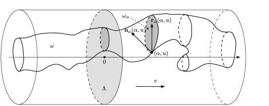
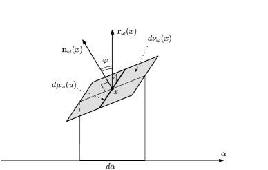
For all $x=(\alpha,u)\in\partial\omega$ where they exist, define the normal vector ${\mathbf{n}}_{\omega}(x)={\mathbf{n}}_{\omega}(\alpha,u)\in{\mathbb{S}}^{d-1}$ pointing inside the domain $\omega$ and the vector ${\mathbf{r}}_{\omega}(x)={\mathbf{r}}_{\omega}(\alpha,u)\in{\mathbb{S}}^{d-2}$ which is the normal vector at $u\in\partial\omega_{\alpha}$ pointing inside the domain $\omega_{\alpha}$ (in fact, ${\mathbf{r}}_{\omega}$ is the normalized projection of ${\mathbf{n}}_{\omega}$ onto ${\mathbb{R}}^{d-1}$) (see Figure 1). Denote also

$$\kappa_{x}=\kappa_{\alpha,u}={\mathbf{n}}_{\omega}(x)\cdot{\mathbf{r}}_{\omega}(x).$$

Observe that $\kappa$ also depends on $\omega$, but we prefer not to write it explicitly in order not to overload the notation. Define the set of regular points

$${\mathcal{R}}_{\omega}=\{x\in\partial\omega\dvtx\partial\omega\mbox{ is continuously differentiable in }x,|{\mathbf{n}}_{\omega}(x)\cdot e|\neq 1\}.$$

Note that $\kappa_{x}\in(0,1]$ for all $x\in{\mathcal{R}}_{\omega}$. Clearly, it holds that

$$d\nu^{\omega}(\alpha,u)=\kappa_{\alpha,u}^{-1}\,d\mu^{\omega}_{\alpha}(u)\,d\alpha$$ (2)

(see Figure 2).

Figure 2: On formula (2); note that $\kappa_{\alpha,u}=\cos\phi$.

We suppose that the following condition holds:

Condition R.

We have $\nu^{\omega}(\partial\omega\setminus{\mathcal{R}}_{\omega})=0$, ${\mathbb{P}}$-a.s.

We say that $y\in\bar{\omega}$ is seen from $x\in\bar{\omega}$ if there exists $h\in{\mathbb{S}}^{d-1}$ and $t_{0}>0$ such that $x+th\in\omega$ for all $t\in(0,t_{0})$ and $x+t_{0}h=y$. Clearly, if $y$ is seen from $x$, then $x$ is seen from $y$, and we write “$x\stackrel{{\scriptstyle\omega}}{{\leftrightarrow}}y$” when this occurs.

One of the main objects of study in this paper is the Knudsen random walk (KRW) $\xi=(\xi_{n})_{n\in{\mathbb{N}}}$ which is a discrete time Markov process on $\partial\omega$ (cf. CPSV1 ). It is defined through its transition density $K$: for $x,y\in\partial\omega$,

$$K(x,y)=\gamma_{d}\frac{((y-x)\cdot{\mathbf{n}}_{\omega}(x))((x-y)\cdot{\mathbf{n}}_{\omega}(y))}{\|x-y\|^{d+1}}{\mathbb{I}}{\{x,y\in{\mathcal{R}}_{\omega},x\stackrel{{\scriptstyle\omega}}{{\leftrightarrow}}y\}},$$ (3)

where $\gamma_{d}=(\int_{{\mathbb{S}}_{e}}h\cdot e\,dh)^{-1}$ is the normalizing constant. This means that, being ${\mathtt{P}}_{\omega},{\mathtt{E}}_{\omega}$ the quenched (i.e., with fixed $\omega$) probability and expectation, for any $x\in{\mathcal{R}}_{\omega}$ and any measurable $B\subset\partial\omega$ we have

$${\mathtt{P}}_{\omega}[\xi_{n+1}\in B\mid\xi_{n}=x]=\int_{B}K(x,y)\,d\nu^{\omega}(y).$$

Following CPSV1 , we shortly explain why this Markov chain is of natural interest. From $\xi_{n}=x$, the next step $\xi_{n+1}=y$ is performed by picking randomly the direction $h=(y-x)/\|y-x\|$ of the step according to Knudsen’s cosine density $\gamma_{d}h\cdot{\mathbf{n}}_{\omega}(x)\,dh$ on the half unit-sphere looking toward the interior of the domain. By elementary geometric considerations, one can check that $d\nu^{\omega}(y)=(h\cdot{\mathbf{n}}_{\omega}(y))^{-1}\|y-x\|^{d-1}\,dh$ and recover the previous formulas.

Let us define also

$$\Phi(\alpha,u,\beta,v)=(\kappa_{\alpha,u}\kappa_{\beta,v})^{-1}K((\alpha,u),(\beta,v)).$$ (4)

From (3) we see that $K(\cdot,\cdot)$ is symmetric, that is, $K(x,y)=K(y,x)$ for all $x,y\in{\mathcal{R}}_{\omega}$; consequently, $\Phi$ has this property as well:

$$\Phi(\alpha,u,\beta,v)=\Phi(\beta,v,\alpha,u)\qquad\mbox{for all }\alpha,\beta\in{\mathbb{R}},u\in\partial\omega_{\alpha},v\in\partial\omega_{\beta}.$$ (5)

Clearly, both $K$ and $\Phi$ depend on $\omega$ as well, but we usually do not indicate this in the notation in order to keep them simple. When we have to do it, we write $K^{\omega},\Phi^{\omega}$ instead of $K,\Phi$. For any $\gamma$ we have

$$\Phi^{\theta_{\gamma}\omega}(\alpha,u,\beta,v)=\Phi^{\omega}(\alpha+\gamma,u,\beta+\gamma,v).$$ (6)

Moreover, the symmetry implies that

$$K^{\omega}((0,u),y) = K^{\theta_{y\cdot e}\omega}\bigl{(}(0,{\mathcal{U}}y),(-y\cdot e,u)\bigr{)},$$ (7)

$$\Phi^{\omega}(0,u,\alpha,v) = \Phi^{\theta_{\alpha}\omega}(0,v,-\alpha,u).$$ (8)

We need also to assume the following technical condition:

Condition P.

There exist constants $N,\varepsilon,\delta$ such that for ${\mathbb{P}}$-almost every $\omega$, for any $x,y\in{\mathcal{R}}_{\omega}$ with $|(x-y)\cdot e|\leq 2$ there exist $B_{1},\ldots,B_{n}\subset\partial\omega$, $n\leq N-1$ with $\nu^{\omega}(B_{i})\geq\delta$ for all $i=1,\ldots,n$ and such that:

• $K(x,z)\geq\varepsilon$ for all $z\in B_{1}$,

• $K(y,z)\geq\varepsilon$ for all $z\in B_{n}$,

• $K(z,z^{\prime})\geq\varepsilon$ for all $z\in B_{i}$, $z^{\prime}\in B_{i+1}$, $i=1,\ldots,n-1$

[if $N=1$ we only require that $K(x,y)\geq\varepsilon$]. In other words, there exists a “thick” path of length at most $N$ joining $x$ and $y$.

Now, following CPSV1 , we define also the Knudsen stochastic billiard (KSB) $(X,V)$. First, we do that for the process starting on the boundary $\partial\omega$ from the point $x_{0}\in{\mathcal{R}}_{\omega}\subset\partial\omega$. Let $x_{0}=\xi_{0},\xi_{1},\xi_{2},\xi_{3},\ldots$ be the trajectory of the random walk, and define

$$\tau_{n}=\sum_{k=1}^{n}\|\xi_{k}-\xi_{k-1}\|.$$

Then, for $t\in[\tau_{n},\tau_{n+1})$, define

$$X_{t}=\xi_{n}+(\xi_{n+1}-\xi_{n})\frac{t-\tau_{n}}{\|\xi_{n+1}-\xi_{n}\|}.$$

The quantity $X_{t}$ stands for the position of the particle at time $t$. Since $(X_{t})_{t\geq 0}$ is not a Markov process by itself, we define also the càdlàg version of the motion direction at time $t$,

$$V_{t}=\lim_{\varepsilon\downarrow 0}\frac{X_{t+\varepsilon}-X_{t}}{\varepsilon}.$$

Then, $V_{t}\in{\mathbb{S}}^{d-1}$ and the couple $(X_{t},V_{t})_{t\geq 0}$ is a Markov process. Of course, we can define also the stochastic billiard starting from the interior of $\omega$ by specifying its initial position $X_{0}$ and initial direction $V_{0}$.

Define

$${\mathfrak{S}}=\{(\omega,u)\dvtx\omega\in\Omega,u\in\partial\omega_{0}\}.$$

One of the most important objects in this paper is the probability measure ${\mathbb{Q}}$ on ${\mathfrak{S}}$ defined by

$$d{\mathbb{Q}}(\omega,u)=\frac{1}{{\mathcal{Z}}}\kappa_{0,u}^{-1}\,d\mu^{\omega}_{0}(u)\,d{\mathbb{P}}(\omega),$$ (9)

where ${\mathcal{Z}}=\int_{\Omega}d{\mathbb{P}}\int_{\Lambda}\kappa_{0,u}^{-1}\,d\mu^{\omega}_{0}(u)$ is the normalizing constant. (We will show that ${\mathbb{Q}}$ is the invariant law of the environment seen from the walker.) To see that ${\mathcal{Z}}$ is finite, note that ${\mathcal{Z}}=\int_{\Omega}d{\mathbb{P}}\int_{0}^{1}d\alpha\int_{\Lambda}\kappa_{\alpha,u}^{-1}\,d\mu^{\omega}_{\alpha}(u)$ by translation invariance, that is, the expected surface area of the tube restricted to the slab $[0,1]\times{\mathbb{R}}^{d-1}$ which is finite by Condition L. Let $L^{2}({\mathfrak{S}})$ be the space of ${\mathbb{Q}}$-square integrable functions $f\dvtx{\mathfrak{S}}\mapsto{\mathbb{R}}$. We use the notation $\langle f\rangle_{{\mathbb{Q}}}$ for the ${\mathbb{Q}}$-expectation of $f$:

$$\langle f\rangle_{{\mathbb{Q}}}=\frac{1}{{\mathcal{Z}}}\int_{\Omega}d{\mathbb{P}}\int_{\Lambda}d\mu^{\omega}_{0}(u)\,\kappa_{0,u}^{-1}f(\omega,u)$$

and we define the scalar product $\langle\cdot,\cdot\rangle_{{\mathbb{Q}}}$ in $L^{2}({\mathfrak{S}})$ by

$$\langle f,g\rangle_{{\mathbb{Q}}}=\frac{1}{{\mathcal{Z}}}\int_{\Omega}d{\mathbb{P}}\int_{\Lambda}d\mu^{\omega}_{0}(u)\,\kappa_{0,u}^{-1}f(\omega,u)g(\omega,u).$$ (10)

Note that $\langle f\rangle_{{\mathbb{Q}}}=\langle{\mathbf{1}},f\rangle_{{\mathbb{Q}}}$ where ${\mathbf{1}}(\omega,u)=1$ for all $\omega,u$.

Now, for $(\beta,u)\in{\mathcal{R}}_{\omega}$ we define the local drift and the second moment of the jump projected on the horizontal direction:

$$\Delta_{\beta}(\omega,u) = {\mathtt{E}}_{\omega}\bigl{(}(\xi_{1}-\xi_{0})\cdot e\mid\xi_{0}=(\beta,u)\bigr{)}$$

$$= \int_{\partial\omega}(x\cdot e-\beta)K((\beta,u),x)\,d\nu^{\omega}(x)$$

$$= \int_{-\infty}^{+\infty}(\alpha-\beta)\,d\alpha\int_{\Lambda}d\mu^{\omega}_{\alpha}(v)\,\kappa_{\beta,u}\Phi(\beta,u,\alpha,v),$$

$$b_{\beta}(\omega,u) = {\mathtt{E}}_{\omega}\bigl{(}\bigl{(}(\xi_{1}-\xi_{0})\cdot e\bigr{)}^{2}\mid\xi_{0}=(\beta,u)\bigr{)}$$

$$= \int_{\partial\omega}(x\cdot e-\beta)^{2}K((\beta,u),x)\,d\nu^{\omega}(x)$$

$$= \int_{-\infty}^{+\infty}(\alpha-\beta)^{2}\,d\alpha\int_{\Lambda}d\mu^{\omega}_{\alpha}(v)\,\kappa_{\beta,u}\Phi(\beta,u,\alpha,v).$$

When $\beta=0$, we write simply $\Delta(\omega,u)$ and $b(\omega,u)$ instead of $\Delta_{0}(\omega,u)$ and $b_{0}(\omega,u)$. In Section 3 we show that $\langle\Delta\rangle_{{\mathbb{Q}}}=0$ [see (3.3)].

Let $Z^{(m)}_{\cdot}$ be the polygonal interpolation of $n/m\mapsto m^{-1/2}\xi_{n}\cdot e$. Our main result is the quenched invariance principle for the horizontal projection of the random walk.

Theorem 2.1

Assume Conditions L, P, R, and suppose that

$$\langle b\rangle_{{\mathbb{Q}}}<\infty.$$ (12)

Then, there exists a constant $\sigma>0$ such that for ${\mathbb{P}}$-almost all $\omega$, for any starting point from ${\mathcal{R}}_{\omega}$, $\sigma^{-1}Z^{(m)}_{\cdot}$ converges in law, under ${\mathtt{P}}_{\omega}$, to Brownian motion as $m\to\infty$.

The constant $\sigma$ is defined by (47) below. Next, we obtain the corresponding result for the continuous time Knudsen stochastic billiard. Define ${\hat{Z}}_{t}^{(s)}=s^{-1/2}X_{st}\cdot e$. Recall also a notation from CPSV1 : for $x\in\omega$, $v\in{\mathbb{S}}^{d-1}$, define (with the convention $\inf\varnothing=\infty$)

$${\mathsf{h}}_{x}(v)=x+v\inf\{t>0\dvtx x+tv\in\partial\omega\}\in\{\partial\omega,\infty\}$$

so that ${\mathsf{h}}_{x}(v)$ is the next point where the particle hits the boundary when starting at the location $x$ with the direction $v$.

Theorem 2.2

Assume Conditions L, P, R, and suppose that (12) holds. Denote

$${\hat{\sigma}}=\frac{\sigma\Gamma({d}/{2}+1){\mathcal{Z}}}{\pi^{1/2}\Gamma(({d+1})/{2})d}\biggl{(}\int_{\Omega}|\omega_{0}|\,d{\mathbb{P}}\biggr{)}^{-1},$$

where $\sigma$ is from Theorem 2.1. Then, for ${\mathbb{P}}$-almost all $\omega$, for any initial conditions $(x_{0},v_{0})$ such that ${\mathsf{h}}_{x_{0}}(v_{0})\in{\mathcal{R}}_{\omega}$, ${\hat{\sigma}}^{-1}{\hat{Z}}^{(s)}_{\cdot}$ converges in law to Brownian motion as $s\to\infty$.

Next, we discuss the question of validity of (12).

Proposition 2.1.

If $d\geq 3$ then (12) holds.

If $d=2$, then one cannot expect (12) to be valid in the situation when $\omega$ contains an infinite straight cylinder. Indeed, we have the following:

Proposition 2.2.

In the two-dimensional case, suppose that there exists an interval $S\subset\Lambda$ such that ${\mathbb{R}}\times S\subset\omega$ for ${\mathbb{P}}$-a.a. $\omega$. Then $\langle b\rangle_{{\mathbb{Q}}}=\infty$.

On the other hand, with $R_{\alpha}(\omega,u)=\sup\{|\alpha-\beta|;(\beta,v)\stackrel{{\scriptstyle\omega}}{{\leftrightarrow}}(\alpha,u)\}$, it is clear that (12) holds when $R_{0}(\omega,u)\leq\mbox{{const}}$ for all $u\in\omega_{0}$, ${\mathbb{P}}$-a.s. Such an example is given by the tube $\{(\alpha,u)\in{\mathbb{R}}^{2}\dvtx\cos\alpha\leq u\leq\cos\alpha+1\}$, a random shift to make it stationary and ergodic (but not mixing).

Remark 2.1.

(i) The continuity assumption of the map $\alpha\mapsto\omega_{\alpha}$ has a geometric meaning: it prevents the tube from having “vertical walls” of nonzero surface measure. The reader may wonder what happens without it. First, the disintegration formula (2) of the surface measure $\nu^{\omega}$ on $\partial\omega$ becomes a product $d{\bar{\mu}}^{\omega}_{\alpha}(u)\,d\phi^{\omega}(\alpha)$ where ${\bar{\mu}}^{\omega}_{\alpha}$ is a measure on the section of $\partial\omega$ by the vertical hyperplane at $\alpha$ and where $d\phi^{\omega}(\alpha)=\kappa_{\alpha,u}^{-1}\,d\alpha+d\phi^{\omega}_{\mathrm{s}}(\alpha)$ with a singular part $\phi^{\omega}_{\mathrm{s}}$. If the singular part has atoms, one can see that the invariant law ${\mathbb{Q}}$ [see (9) above] of the environment seen from the particle has a marginal in $\omega$ which is singular with respect to ${\mathbb{P}}$. This happens because, if the vertical walls constitute a positive proportion of the tube’s surface, in the equilibrium the particle finds itself on a vertical wall with positive probability; on the other hand, if $\omega$ has the law ${\mathbb{P}}$, a.s. there is no vertical wall at the origin. The general situation is interesting but complicated; in any case, our results continue to be valid in this situation as well [an important observation is that (3.4) below would still hold, possibly with another constant]. To keep things simple, we will consider only, all through the paper, random tubes satisfying the continuity assumption. In the Appendix, we discuss the general case in more detail. Another possible approach to this general case is to work with the continuous-time stochastic billiard directly (cf. Section 3.2).

(ii) A particular example of tubes is given by rotation invariant tubes. They are obtained by rotating around the first axis the graph of a positive bounded function. The main simplification is that, with the proper formalism, one can forget the transverse component $u$. Then the problem becomes purely one-dimensional.

3 Environment viewed from the particle and the construction of the corrector

3.1 Environment viewed from the particle: Discrete case

One of the main methods we use in this paper is considering the environment $\omega$ seen from the current location of the random walk. The “environment viewed from the particle” is the Markov chain

$$\bigl{(}(\theta_{\xi_{n}\cdot e}\omega,{\mathcal{U}}\xi_{n}),n=0,1,2,\ldots\bigr{)}$$

with state space ${\mathfrak{S}}$. The transition operator $G$ for this process acts on functions $f\dvtx{\mathfrak{S}}\mapsto{\mathbb{R}}$ as follows [cf. (2) and (4)]:

$$Gf(\omega,u) = {\mathtt{E}}_{\omega}\bigl{(}f(\theta_{\xi_{1}\cdot e}\omega,{\mathcal{U}}\xi_{1})\mid\xi_{0}=(0,u)\bigr{)}$$

$$= \int_{\partial\omega}K((0,u),x)f(\theta_{x\cdot e}\omega,{\mathcal{U}}x)\,d\nu^{\omega}(x)$$

$$= \int_{-\infty}^{+\infty}d\alpha\int_{\Lambda}d\mu^{\omega}_{\alpha}(v)\,\kappa_{0,u}f(\theta_{\alpha}\omega,v)\Phi(0,u,\alpha,v).$$

Remark 3.1.

Note that our environment consists not only of the tube with an appropriate horizontal shift, but also of the transverse component of the walk. Another possible choice for the environment would be obtained by rotating the shifted tube to make it pass through the origin with inner normal at this point given by the last coordinate vector. However, we made the present choice to keep notation simple.

Next, we show that this new Markov chain is reversible with reversible measure ${\mathbb{Q}}$ given by (9), which means that $G$ is a self-adjoint operator in $L^{2}({\mathfrak{S}})=L^{2}({\mathfrak{S}},{\mathbb{Q}})$:

Lemma 3.1

For all $f,g\in L^{2}({\mathfrak{S}})$ we have $\langle g,Gf\rangle_{{\mathbb{Q}}}=\langle f,Gg\rangle_{{\mathbb{Q}}}$. Hence, the law ${\mathbb{Q}}$ is invariant for the Markov chain of the environment viewed from the particle which means that for any $f\in L^{2}({\mathfrak{S}})$ and all $n$,

$$\langle{\mathtt{E}}_{\omega}[f(\theta_{\xi_{n}\cdot e}\omega,{\mathcal{U}}\xi_{n})\mid\xi_{0}=(0,u)]\rangle_{{\mathbb{Q}}}=\langle f\rangle_{{\mathbb{Q}}}.$$ (14)

Indeed, from (9) and (3.1),

$$\quad\langle g,Gf\rangle_{{\mathbb{Q}}} = \frac{1}{{\mathcal{Z}}}\int_{\Omega}d{\mathbb{P}}\int_{\Lambda}d\mu^{\omega}_{0}(u)\,g(\omega,u)\kappa_{0,u}^{-1}\int_{-\infty}^{+\infty}d\alpha$$

$${}\times\int_{\Lambda}d\mu^{\omega}_{\alpha}(v)\,\kappa_{0,u}\Phi(0,u,\alpha,v)f(\theta_{\alpha}\omega,v)$$

$$= \frac{1}{{\mathcal{Z}}}\int_{-\infty}^{+\infty}d\alpha\int_{\Omega}d{\mathbb{P}}\int_{\Lambda^{2}}d\mu^{\omega}_{0,\alpha}(u,v)\,g(\omega,u)f(\theta_{\alpha}\omega,v)\Phi(0,u,\alpha,v)$$

$$= \frac{1}{{\mathcal{Z}}}\int_{-\infty}^{+\infty}d\alpha\int_{\Omega}d{\mathbb{P}}\int_{\Lambda^{2}}d\mu^{\theta_{\alpha}\omega}_{-\alpha,0}(u,v)\,g(\omega,u)f(\theta_{\alpha}\omega,v)$$

$$\hskip 96.7pt{}\times\Phi^{\theta_{\alpha}\omega}(-\alpha,u,0,v)$$

$$= \frac{1}{{\mathcal{Z}}}\int_{-\infty}^{+\infty}d\alpha\int_{\Omega}d{\mathbb{P}}\int_{\Lambda^{2}}d\mu^{\omega}_{-\alpha,0}(u,v)\,g(\theta_{-\alpha}\omega,u)f(\omega,v)$$

$$\hskip 96.7pt{}\times\Phi(-\alpha,u,0,v)$$

$$= \frac{1}{{\mathcal{Z}}}\int_{\Omega}d{\mathbb{P}}\int_{\Lambda}d\mu^{\omega}_{0}(v)\,f(\omega,v)\kappa_{0,v}^{-1}\int_{-\infty}^{+\infty}d\alpha$$

$${}\times\int_{\Lambda}d\mu^{\omega}_{-\alpha}(u)\,\kappa_{0,v}\Phi(0,v,-\alpha,u)g(\theta_{-\alpha}\omega,u)$$

$$= \langle f,Gg\rangle_{{\mathbb{Q}}},$$

where we used (6) to pass from (3.1) to (3.1), the translation invariance of ${\mathbb{P}}$ to pass from (3.1) to (3.1), the symmetry property (5) to pass from (3.1) to (3.1) and the change of variable $\alpha\mapsto-\alpha$ to obtain the last line.

Let us define a semi-definite scalar product $\langle g,f\rangle_{1}:=\langle g,(I-G)f\rangle_{{\mathbb{Q}}}$. Again using (3.1), the translation invariance of ${\mathbb{P}}$ and the symmetry of $\Phi$, we obtain

$$\langle g,f\rangle_{1} = \frac{1}{{\mathcal{Z}}}\int_{-\infty}^{+\infty}d\alpha\int_{\Omega}d{\mathbb{P}}\int_{\Lambda^{2}}d\mu^{\omega}_{0,\alpha}(u,v)\,\Phi(0,u,\alpha,v)$$

$$\hskip 97.74pt{}\times g(\omega,u)\bigl{(}f(\omega,u)-f(\theta_{\alpha}\omega,v)\bigr{)}$$

$$= \frac{1}{{\mathcal{Z}}}\int_{-\infty}^{+\infty}d\alpha\int_{\Omega}d{\mathbb{P}}\int_{\Lambda^{2}}d\mu^{\omega}_{-\alpha,0}(u,v)\,\Phi(-\alpha,u,0,v)$$

$$\hskip 97.74pt{}\times g(\theta_{-\alpha}\omega,u)\bigl{(}f(\theta_{-\alpha}\omega,u)-f(\omega,v)\bigr{)}$$

$$= \frac{1}{{\mathcal{Z}}}\int_{-\infty}^{+\infty}d\alpha\int_{\Omega}d{\mathbb{P}}\int_{\Lambda^{2}}d\mu^{\omega}_{0,\alpha}(u,v)\,\Phi(0,u,\alpha,v)$$

$$\hskip 97.74pt{}\times g(\theta_{\alpha}\omega,v)\bigl{(}f(\theta_{\alpha}\omega,v)-f(\omega,u)\bigr{)}.$$

Consequently,

$$\langle g,f\rangle_{1} = \frac{1}{2{\mathcal{Z}}}\int_{-\infty}^{+\infty}d\alpha\int_{\Omega}d{\mathbb{P}}\int_{\Lambda^{2}}d\mu^{\omega}_{0,\alpha}(u,v)\,\Phi(0,u,\alpha,v)\bigl{(}f(\omega,u)-f(\theta_{\alpha}\omega,v)\bigr{)}\hskip 1.5pt$$

$$\hskip 101.5pt{}\times\bigl{(}g(\omega,u)-g(\theta_{\alpha}\omega,v)\bigr{)},\hskip 1.5pt$$

so the Dirichlet form $\langle f,f\rangle_{1}$ can be explicitly written as

$$\langle f,f\rangle_{1} = \frac{1}{2{\mathcal{Z}}}\int_{-\infty}^{+\infty}d\alpha\int_{\Omega}d{\mathbb{P}}\int_{\Lambda^{2}}d\mu^{\omega}_{0,\alpha}(u,v)\,\Phi(0,u,\alpha,v)$$

$$\hskip 102.5pt{}\times\bigl{(}f(\omega,u)-f(\theta_{\alpha}\omega,v)\bigr{)}^{2},$$

or, by (2) and (4),

$$\langle f,f\rangle_{1} = \frac{1}{2{\mathcal{Z}}}\int_{\Omega}d{\mathbb{P}}\int_{\Lambda}\kappa_{0,u}^{-1}\,d\mu^{\omega}_{0}(u)$$

$${}\times\int_{\partial\omega}d\nu^{\omega}(x)\,K((0,u),x)\bigl{(}f(\omega,u)-f(\theta_{x\cdot e}\omega,{\mathcal{U}}x)\bigr{)}^{2}.$$

At this point it is convenient to establish the following result:

Lemma 3.2

The Markov process with initial law ${\mathbb{Q}}$ and transition operator $G$ is ergodic.

Suppose that $f\in L^{2}({\mathfrak{S}})$ is such that $f=Gf$. Then $\langle f,f\rangle_{1}=0$ and so, by the translation invariance and (3.1),

$$\int_{\Omega}d{\mathbb{P}}\int_{\Lambda}\kappa_{s,u}^{-1}\,d\mu^{\omega}_{s}(u)\int_{\partial\omega}d\nu^{\omega}(x)\,K((s,u),x)\bigl{(}f(\theta_{s}\omega,u)-f(\theta_{x\cdot e}\omega,{\mathcal{U}}x)\bigr{)}^{2}=0$$

for any $s$. Integrating the above equation in $s$ and using (2), we obtain

$$\int_{\Omega}d{\mathbb{P}}\int_{(\partial\omega)^{2}}d\nu^{\omega}(x)\,d\nu^{\omega}(y)\,K(x,y)\bigl{(}f(\theta_{x\cdot e}\omega,{\mathcal{U}}x)-f(\theta_{y\cdot e}\omega,{\mathcal{U}}y)\bigr{)}^{2}=0.$$ (21)

Let us recall Lemma 3.3(iii) from CPSV1 : if for some $x,y\in{\mathcal{R}}_{\omega}$ we have $K(x,y)>0$, then there exist $\delta>0$ and two neighborhoods $B_{x}$ of $x$ and $B_{y}$ of $y$ such that $K(x^{\prime},y^{\prime})>\delta$ for all $x^{\prime}\in B_{x},y^{\prime}\in B_{y}$. Now, for such $x,y$, (21) implies that there exists a constant ${\hat{c}}(\omega,x,y)$ such that $f(\theta_{z\cdot e}\omega,{\mathcal{U}}z)={\hat{c}}(\omega,x,y)$ for $\nu^{\omega}$-almost all $z\in B_{x}\cup B_{y}$. By the irreducibility Condition P (in fact, a much weaker irreducibility condition would be sufficient), this implies that $f(\theta_{z\cdot e}\omega,{\mathcal{U}}z)={\hat{c}}(\omega)$ for $\nu^{\omega}$-almost all $z\in{\mathcal{R}}_{\omega}$. Since ${\mathbb{P}}$ is ergodic, this means that $f(\omega,u)={\hat{c}}$ for $\mu^{\omega}_{0}$-almost all $u$ and ${\mathbb{P}}$-almost all $\omega$.

3.2 Environment viewed from the particle: Continuous case

For the sake of completeness, we present also an analogous result for the Knudsen stochastic billiard $(X_{t},V_{t})$. The notation and the results of this section will not be used in the rest of this paper.

Let $\widehat{\mathfrak{S}}=\{(\omega,u)\dvtx\omega\in\Omega,u\in\omega_{0}\}$, and let ${\widehat{\mathbb{Q}}}$ be the probability measure on $\widehat{\mathfrak{S}}\times{\mathbb{S}}^{d-1}$ defined by

$$d{\widehat{\mathbb{Q}}}(\omega,u,h)=\frac{1}{{\widehat{\mathcal{Z}}}}{\mathbb{I}}{\{u\in\omega_{0}\}}\,du\,dh\,d{\mathbb{P}}(\omega),$$

where ${\widehat{\mathcal{Z}}}=|{\mathbb{S}}^{d-1}|\int_{\Omega}|\omega_{0}|d{\mathbb{P}}$ is the normalizing constant. The scalar product $\langle\cdot,\cdot\rangle_{{\widehat{\mathbb{Q}}}}$ in $L^{2}({\widehat{\mathbb{Q}}})$ is given, for two ${\widehat{\mathbb{Q}}}$-square integrable functions ${\hat{f}},{\hat{g}}\dvtx\widehat{\mathfrak{S}}\times{\mathbb{S}}^{d-1}\mapsto{\mathbb{R}}$, by

$$\langle{\hat{f}},{\hat{g}}\rangle_{{\widehat{\mathbb{Q}}}}=\frac{1}{{\widehat{\mathcal{Z}}}}\int_{\Omega}d{\mathbb{P}}\int_{\omega_{0}}du\int_{{\mathbb{S}}^{d-1}}dh\,{\hat{f}}(\omega,u,h){\hat{g}}(\omega,u,h).$$

For the continuous time KSB, the “environment viewed from the particle” is the Markov process $((\theta_{X_{t}\cdot e}\omega,{\mathcal{U}}X_{t},V_{t}),t\geq 0)$ with the state space $\widehat{\mathfrak{S}}\times{\mathbb{S}}^{d-1}$. The transition semi-group ${\widehat{\mathcal{P}}}_{t}$ for this process acts on functions ${\hat{f}}\dvtx\widehat{\mathfrak{S}}\times{\mathbb{S}}^{d-1}\mapsto{\mathbb{R}}$ in the following way:

$${\widehat{\mathcal{P}}}_{t}{\hat{f}}(\omega,u,h)={\mathtt{E}}_{\omega}\bigl{(}{\hat{f}}(\theta_{X_{t}\cdot e}\omega,{\mathcal{U}}X_{t},V_{t})\mid X_{0}=(0,u),V_{0}=h\bigr{)}.$$

We show that ${\widehat{\mathcal{P}}}$ is quasi-reversible with respect to the law ${\widehat{\mathbb{Q}}}$.

Lemma 3.3

For all ${\hat{f}},{\hat{g}}\in L^{2}({\widehat{\mathbb{Q}}})$ and $t>0$ we have

$$\langle{\hat{g}},{\widehat{\mathcal{P}}}_{t}{\hat{f}}\rangle_{{\widehat{\mathbb{Q}}}}=\langle{\breve{f}},{\widehat{\mathcal{P}}}_{t}{\breve{g}}\rangle_{{\widehat{\mathbb{Q}}}}$$ (22)

with $\breve{f}(\omega,u,h)=\hat{f}(\omega,u,-h)$. In particular, the law ${\widehat{\mathbb{Q}}}$ is invariant for the process $((\theta_{X_{t}\cdot e}\omega,{\mathcal{U}}X_{t},V_{t}),t\geq 0)$.

We first prove that (22) implies that the law ${\widehat{\mathbb{Q}}}$ is invariant. Indeed, taking ${\hat{g}}={\mathbf{1}}$, we get for all test functions ${\hat{f}}$

$$\langle{\mathbf{1}},{\widehat{\mathcal{P}}}_{t}{\hat{f}}\rangle_{{\widehat{\mathbb{Q}}}} = \langle{\breve{f}},{\mathbf{1}}\rangle_{{\widehat{\mathbb{Q}}}}$$

$$= \langle{f},{\mathbf{1}}\rangle_{{\widehat{\mathbb{Q}}}}$$

by the change of variable $h$ into $-h$ in the integral. Hence ${\widehat{\mathbb{Q}}}$ is invariant.

We now turn to the proof of (22). Introducing the notation ${\mathtt{P}}_{t}^{\omega}$ for the transition kernel of KSB,

$${\mathtt{P}}_{\omega}(X_{t}\in dx^{\prime},V_{t}\in dh^{\prime}\mid X_{0}=x,V_{0}=h)={\mathtt{P}}_{t}^{\omega}(x,h;x^{\prime},h^{\prime})\,dx^{\prime}\,dh^{\prime},$$

we observe that

$${\widehat{\mathcal{P}}}_{t}{\hat{f}}(\omega,u,h)=\int_{\omega}dx^{\prime}\int_{{\mathbb{S}}^{d-1}}dh^{\prime}\,{\mathtt{P}}_{t}^{\omega}((0,u),h;x^{\prime},h^{\prime}){\hat{f}}(\theta_{x^{\prime}\cdot e},\omega,{\mathcal{U}}x^{\prime},h^{\prime}).$$

In Theorem 2.5 in CPSV1 , it was shown that ${\mathtt{P}}_{t}^{\omega}$ is itself quasi-reversible, that is,

$${\mathtt{P}}_{t}^{\omega}(x,h;x^{\prime},h^{\prime})={\mathtt{P}}_{t}^{\omega}(x^{\prime},-h^{\prime};x,-h).$$

Therefore,

$$\langle{\hat{g}},{\widehat{\mathcal{P}}}_{t}{\hat{f}}\rangle_{{\widehat{\mathbb{Q}}}} = \frac{1}{{\widehat{\mathcal{Z}}}}\int_{\Omega}d{\mathbb{P}}\int_{\omega_{0}}du\int_{{\mathbb{S}}^{d-1}}dh\,{\hat{g}}(\omega,u,h){\widehat{\mathcal{P}}}_{t}{\hat{f}}(\omega,u,h)$$

$$= \frac{1}{{\widehat{\mathcal{Z}}}}\int_{\Omega}d{\mathbb{P}}\int_{\omega_{0}}du\int_{{\mathbb{S}}^{d-1}}dh\,{\hat{g}}(\omega,u,h)\int_{\mathbb{R}}d\alpha\int_{\omega_{\alpha}}du^{\prime}$$

$${}\times\int_{{\mathbb{S}}^{d-1}}dh^{\prime}\,{\mathtt{P}}_{t}^{\omega}((0,u),h;(\alpha,u^{\prime}),h^{\prime}){\hat{f}}(\theta_{\alpha},\omega,u^{\prime},h^{\prime})$$

$$= \frac{1}{{\widehat{\mathcal{Z}}}}\int_{\Omega}d{\mathbb{P}}\int_{\omega_{0}}du\int_{{\mathbb{S}}^{d-1}}dh\,{\hat{g}}(\omega,u,h)\int_{\mathbb{R}}d\alpha\int_{\omega_{\alpha}}du^{\prime}$$

$${}\times\int_{{\mathbb{S}}^{d-1}}dh^{\prime}\,{{\mathtt{P}}_{t}^{\theta_{\alpha}\omega}{}}((0,u^{\prime}),-h^{\prime};(-\alpha,u),-h){\hat{f}}(\theta_{\alpha}\omega,u^{\prime},h^{\prime})$$

$$= \frac{1}{{\widehat{\mathcal{Z}}}}\int_{\mathbb{R}}d\alpha\int_{\Omega}d{\mathbb{P}}\int_{\omega_{-\alpha}}du\int_{{\mathbb{S}}^{d-1}}dh\,{\hat{g}}(\theta_{-\alpha},\omega,u,h)\int_{\omega_{0}}du^{\prime}$$

$${}\times\int_{{\mathbb{S}}^{d-1}}dh^{\prime}\,{{\mathtt{P}}_{t}^{\omega}{}}((0,u^{\prime}),-h^{\prime};(-\alpha,u),-h){\hat{f}}(\omega,u^{\prime},h^{\prime})$$

$$= \frac{1}{{\widehat{\mathcal{Z}}}}\int_{\mathbb{R}}d\alpha\int_{\Omega}d{\mathbb{P}}\int_{\omega_{\alpha}}du\int_{{\mathbb{S}}^{d-1}}dh\,{\hat{g}}(\theta_{\alpha},\omega,u,-h)\int_{\omega_{0}}du^{\prime}$$

$${}\times\int_{{\mathbb{S}}^{d-1}}dh^{\prime}\,{{\mathtt{P}}_{t}^{\omega}{}}((0,u^{\prime}),h^{\prime};(\alpha,u),h){\hat{f}}(\omega,u^{\prime},-h^{\prime})$$

$$= \langle{\breve{f}},{\widehat{\mathcal{P}}}_{t}{\breve{g}}\rangle_{{\widehat{\mathbb{Q}}}},$$

where we used that the Lebesgue measure on ${\mathbb{R}}^{d}$ is product to get the second line, quasi-reversibility for the third one, Fubini and translation invariance of ${\mathbb{P}}$ for the fourth one, and change of variables $(h,h^{\prime},\alpha)$ to $(-h,-h^{\prime},-\alpha)$ in the fifth one.

3.3 Construction of the corrector

Now, we are going to construct the corrector function for the random walk $\xi$.

Let us show that for any $g\in L^{2}({\mathfrak{S}})$,

$$\langle g,\Delta\rangle_{{\mathbb{Q}}}\leq\tfrac{1}{\sqrt{2}}\langle b\rangle_{{\mathbb{Q}}}^{1/2}\langle g,g\rangle_{1}^{1/2}.$$ (23)

Indeed, from (2) we obtain

$$\langle g,\Delta\rangle_{{\mathbb{Q}}} = \frac{1}{{\mathcal{Z}}}\int_{-\infty}^{+\infty}\alpha\,d\alpha\int_{\Omega}d{\mathbb{P}}\int_{\Lambda^{2}}\mu^{\omega}_{0,\alpha}(u,v)g(\omega,u)\Phi(0,u,\alpha,v)$$

$$= \frac{1}{{\mathcal{Z}}}\int_{-\infty}^{+\infty}\alpha\,d\alpha\int_{\Omega}d{\mathbb{P}}\int_{\Lambda^{2}}\mu^{\omega}_{-\alpha,0}(u,v)g(\theta_{-\alpha}\omega,u)\Phi(-\alpha,u,0,v)$$

$$= -\frac{1}{{\mathcal{Z}}}\int_{-\infty}^{+\infty}\alpha\,d\alpha\int_{\Omega}d{\mathbb{P}}\int_{\Lambda^{2}}\mu^{\omega}_{0,\alpha}(u,v)g(\theta_{\alpha}\omega,v)\Phi(0,u,\alpha,v),$$

so

$$\langle g,\Delta\rangle_{{\mathbb{Q}}} = \frac{1}{2{\mathcal{Z}}}\int_{-\infty}^{+\infty}\alpha\,d\alpha\int_{\Omega}d{\mathbb{P}}$$

$${}\times\int_{\Lambda^{2}}\mu^{\omega}_{0,\alpha}(u,v)\Phi(0,u,\alpha,v)\bigl{(}g(\omega,u)-g(\theta_{\alpha}\omega,v)\bigr{)}.$$

Using the Cauchy–Schwarz inequality in (3.3), we obtain

$$\langle g,\Delta\rangle_{{\mathbb{Q}}} \leq \frac{1}{2}\biggl{[}\frac{1}{{\mathcal{Z}}}\int_{-\infty}^{+\infty}\alpha^{2}\,d\alpha\int_{\Omega}d{\mathbb{P}}\int_{\Lambda^{2}}\mu^{\omega}_{0,\alpha}(u,v)\Phi(0,u,\alpha,v)$$

$$\hskip 11.0pt{}\times\frac{1}{{\mathcal{Z}}}\int_{-\infty}^{+\infty}d\alpha\int_{\Omega}d{\mathbb{P}}\int_{\Lambda^{2}}\mu^{\omega}_{0,\alpha}(u,v)\Phi(0,u,\alpha,v)$$

$$\hskip 120.6pt{}\times\bigl{(}g(\omega,u)-g(\theta_{\alpha}\omega,v)\bigr{)}^{2}\biggr{]}^{1/2}$$

$$= \frac{1}{2}\langle b\rangle_{{\mathbb{Q}}}^{1/2}(2\langle g,g\rangle_{1})^{1/2},$$

which shows (23).

Note that, from (3.3) with $g=1$ we obtain the important property

$$\langle\Delta\rangle_{{\mathbb{Q}}}=0.$$

As shown in Chapter 1 of KLO , we have the variational formula

$$\langle(I-G)^{-1/2}\Delta,(I-G)^{-1/2}\Delta\rangle_{{\mathbb{Q}}} = \langle\Delta,(I-G)^{-1}\Delta\rangle_{{\mathbb{Q}}}$$

$$= \sup\{\langle g,\Delta\rangle_{{\mathbb{Q}}}-\langle g,g\rangle_{1},\langle g,g\rangle_{1}<\infty\}.$$

Then provided that (12) holds, inequality (23) implies that the drift $\Delta$ belongs to the range of $(I-G)^{1/2}$, and so the time-variance of $\Delta$ is finite. At this point we mention that this already implies weaker forms of the CLT, by applying KV (under the invariant measure, or in probability with respect to the environment) or DFGW (under the annealed measure). With this observation, we could have used the resolvent method originally developed in KV , KLO to construct the corrector. However, it is more direct to use the method of the orthogonal projections on the potential subspace (cf. BP , M , MP ).

For $\omega\in\Omega$, $u\in\partial\omega_{0}$, define

$${\mathsf{V}}^{+}_{\omega,u} = \{y\in\partial\omega\dvtx y\cdot e>0,K((0,u),y)>0\},$$

$${\mathsf{V}}^{-}_{\omega,u} = \{y\in\partial\omega\dvtx y\cdot e<0,K((0,u),y)>0\}.$$

Then, in addition to the space ${\mathfrak{S}}$, we define two spaces ${\mathfrak{N}}\subset{\mathfrak{M}}$ in the following way:

$${\mathfrak{N}} = \{(\omega,u,y)\dvtx\omega\in\Omega,u\in\partial\omega_{0},y\in{\mathsf{V}}^{+}_{\omega,u}\},$$

$${\mathfrak{M}} = \{(\omega,u,y)\dvtx\omega\in\Omega,u\in\partial\omega_{0},y\in\partial\omega\}.$$

On ${\mathfrak{N}}$ we define the measure $K{\mathbb{Q}}$ with mass that is less than 1 for which a nonnegative function $f\dvtx{\mathfrak{N}}\mapsto{\mathbb{R}}$ has the expected value

$$\langle f\rangle_{{K{\mathbb{Q}}}}=\biggl{\langle}\int_{{\mathsf{V}}^{+}_{\omega,u}}f(\omega,u,y)K((0,u),y)\,d\nu^{\omega}(y)\biggr{\rangle}_{{\mathbb{Q}}}.$$ (25)

Two square-integrable functions $f,g\dvtx{\mathfrak{N}}\mapsto{\mathbb{R}}$ have scalar product,

$$\langle f,g\rangle_{{K{\mathbb{Q}}}}=\biggl{\langle}\int_{{\mathsf{V}}^{+}_{\omega,u}}f(\omega,u,y)g(\omega,u,y)K((0,u),y)\,d\nu^{\omega}(y)\biggr{\rangle}_{{\mathbb{Q}}}.$$ (26)

Also, define the gradient $\nabla$ as the map that transfers a function $f\dvtx{\mathfrak{S}}\mapsto{\mathbb{R}}$ to the function $\nabla f\dvtx{\mathfrak{N}}\mapsto{\mathbb{R}}$, defined by

$$(\nabla f)(\omega,u,y)=f(\theta_{y\cdot e}\omega,{\mathcal{U}}y)-f(\omega,u).$$ (27)

Since ${\mathbb{Q}}$ is reversible for $G$, we can write

$$\langle(\nabla f)^{2}\rangle_{{K{\mathbb{Q}}}} = \biggl{\langle}\int_{{\mathsf{V}}^{+}_{\omega,u}}\bigl{(}f(\theta_{y\cdot e}\omega,{\mathcal{U}}y)-f(\omega,u)\bigr{)}^{2}K((0,u),y)\,d\nu^{\omega}(y)\biggr{\rangle}_{{\mathbb{Q}}}$$

$$\leq 2\biggl{\langle}\int_{\partial\omega}f^{2}(\theta_{y\cdot e}\omega,{\mathcal{U}}y)K((0,u),y)\,d\nu^{\omega}(y)\biggr{\rangle}_{{\mathbb{Q}}}$$

$${}+2\biggl{\langle}\int_{\partial\omega}f^{2}(\omega,u)K((0,u),y)\,d\nu^{\omega}(y)\biggr{\rangle}_{{\mathbb{Q}}}$$

$$= 2\langle Gf^{2}\rangle_{{\mathbb{Q}}}+2\langle f^{2}\rangle_{{\mathbb{Q}}}$$

$$= 4\langle f^{2}\rangle_{{\mathbb{Q}}},$$

so $\nabla$ is, in fact, a map from $L^{2}({\mathfrak{S}})$ to $L^{2}({\mathfrak{N}})$.

Then, following BP , we denote by $L^{2}_{\nabla}({\mathfrak{N}})$ the closure of the set of gradients of all functions from $L^{2}({\mathfrak{S}})$. We then consider the orthogonal decomposition of $L^{2}({\mathfrak{N}})$ into the “potential” and the “solenoidal” subspaces: $L^{2}({\mathfrak{N}})=L^{2}_{\nabla}({\mathfrak{N}})\oplus(L^{2}_{\nabla}({\mathfrak{N}}))^{\bot}$. To characterize the solenoidal subspace $(L^{2}_{\nabla}({\mathfrak{N}}))^{\bot}$, we introduce the divergence operator in the following way. For $f\dvtx{\mathfrak{N}}\mapsto{\mathbb{R}}$, we have $\operatorname{div}f\dvtx{\mathfrak{S}}\mapsto{\mathbb{R}}$ defined by

$$(\operatorname{div}f)(\omega,u) = \int_{{\mathsf{V}}^{+}_{\omega,u}}K((0,u),y)f(\omega,u,y)\,d\nu^{\omega}(y)$$

$${}-\int_{{\mathsf{V}}^{-}_{\omega,u}}K((0,u),y)f\bigl{(}\theta_{y\cdot e}\omega,{\mathcal{U}}y,(|y\cdot e|,u)\bigr{)}\,d\nu^{\omega}(y)$$

[note that for $y\in{\mathsf{V}}^{-}_{\omega,u}$ we have $(|y\cdot e|,u)\in{\mathsf{V}}^{+}_{\theta_{y\cdot e}\omega,{\mathcal{U}}y}$]. Now, we verify the following integration by parts formula: for any $f\in L^{2}({\mathfrak{S}})$, $g\in L^{2}({\mathfrak{N}})$,

$$\langle g,\nabla f\rangle_{{K{\mathbb{Q}}}}=-\langle f\operatorname{div}g\rangle_{{\mathbb{Q}}}.$$ (29)

Indeed, we have

$$\quad\langle g,\nabla f\rangle_{{K{\mathbb{Q}}}} = \biggl{\langle}\int_{{\mathsf{V}}^{+}_{\omega,u}}K((0,u),y)g(\omega,u,y)$$

$$\hskip 24.3pt{}\times\bigl{(}f(\theta_{y\cdot e}\omega,{\mathcal{U}}y)-f(\omega,u)\bigr{)}\,d\nu^{\omega}(y)\biggr{\rangle}_{{\mathbb{Q}}}$$

$$= -\biggl{\langle}\int_{{\mathsf{V}}^{+}_{\omega,u}}K((0,u),y)g(\omega,u,y)f(\omega,u)\,d\nu^{\omega}(y)\biggr{\rangle}_{{\mathbb{Q}}}$$

$${}+\biggl{\langle}\int_{{\mathsf{V}}^{+}_{\omega,u}}K((0,u),y)g(\omega,u,y)f(\theta_{y\cdot e}\omega,{\mathcal{U}}y)\,d\nu^{\omega}(y)\biggr{\rangle}_{{\mathbb{Q}}}.$$

For the second term in the right-hand side of (3.3), we obtain

$$\biggl{\langle}\int_{{\mathsf{V}}^{+}_{\omega,u}}K((0,u),y)g(\omega,u,y)f(\theta_{y\cdot e}\omega,{\mathcal{U}}y)\,d\nu^{\omega}(y)\biggr{\rangle}_{{\mathbb{Q}}}$$

$$\qquad=\frac{1}{{\mathcal{Z}}}\int_{\Omega}d{\mathbb{P}}\int_{0}^{+\infty}d\alpha\int_{\Lambda^{2}}d\mu^{\omega}_{0,\alpha}(u,v)\,\Phi(0,u,\alpha,v)g(\omega,u,(\alpha,v))f(\theta_{\alpha}\omega,v)$$

$$\qquad=\frac{1}{{\mathcal{Z}}}\int_{-\infty}^{0}d\alpha\int_{\Omega}d{\mathbb{P}}\int_{\Lambda^{2}}d\mu^{\omega}_{\alpha,0}(v,u)\,\Phi(\alpha,v,0,u)g(\theta_{\alpha}\omega,v,(|\alpha|,u))f(\omega,u)$$

$$\qquad=\biggl{\langle}\int_{{\mathsf{V}}^{-}_{\omega,u}}f(\omega,u)g\bigl{(}\theta_{y\cdot e}\omega,{\mathcal{U}}y,(|y\cdot e|,u)\bigr{)}K((0,u),y)\,d\nu^{\omega}(y)\biggr{\rangle}_{{\mathbb{Q}}},$$

and so

$$\langle g,\nabla f\rangle_{{K{\mathbb{Q}}}} = -\biggl{\langle}\int_{{\mathsf{V}}^{+}_{\omega,u}}g(\omega,u,y)f(\omega,u)K((0,u),y)\,d\nu^{\omega}(y)\biggr{\rangle}_{{\mathbb{Q}}}$$

$${}+\biggl{\langle}\int_{{\mathsf{V}}^{-}_{\omega,u}}f(\omega,u)g\bigl{(}\theta_{y\cdot e}\omega,{\mathcal{U}}y,(|y\cdot e|,u)\bigr{)}K((0,u),y)\,d\nu^{\omega}(y)\biggr{\rangle}_{{\mathbb{Q}}}$$

$$= -\langle f\operatorname{div}g\rangle_{{\mathbb{Q}}}$$

and the proof of (29) is complete.

Analogously to Lemma 4.2 of BP , we can characterize the space $(L^{2}_{\nabla}({\mathfrak{N}}))^{\bot}$ as follows:

Lemma 3.4

$g\in(L^{2}_{\nabla}({\mathfrak{N}}))^{\bot}$ if and only if $\operatorname{div}g(\omega,u)=0$ for ${\mathbb{Q}}$-almost all $(\omega,u)$.

This is a direct consequence of (29).

A function $f\in L^{2}({\mathfrak{N}})$ can be interpreted as a flow by putting formally

$$f(\omega,u,y):=-f\bigl{(}\theta_{y\cdot e}\omega,{\mathcal{U}}y,(|y\cdot e|,u)\bigr{)}$$

for $y\in{\mathsf{V}}^{-}_{\omega,u},\omega\in{\mathfrak{S}}$. Then it is straightforward to obtain that every $f\in L^{2}_{\nabla}({\mathfrak{N}})$ is curl-free, which means that for any loop $y_{0},y_{1},\ldots,y_{n}\in\partial\omega$ with $y_{0}=y_{n}$ and $K(y_{i},y_{i+1})>0$ for $i=1,\ldots,n-1$, we have

$$\sum_{i=0}^{n-1}f\bigl{(}\theta_{y_{i}\cdot e}\omega,{\mathcal{U}}y_{i},y_{i+1}-(y_{i}\cdot e)e\bigr{)}=0.$$ (31)

Every curl-free function $f$ can be integrated into a unique function $\phi\dvtx{\mathfrak{M}}\mapsto{\mathbb{R}}$ which can be defined by

$$\phi(\omega,u,y)=\sum_{i=0}^{n-1}f\bigl{(}\theta_{y_{i}\cdot e}\omega,{\mathcal{U}}y_{i},y_{i+1}-(y_{i}\cdot e)e\bigr{)},$$ (32)

where $y_{0},y_{1},\ldots,y_{n}\in\partial\omega$ is an arbitrary path such that $y_{0}=(0,u)$, $y_{n}=y$, and $K(y_{i},y_{i+1})>0$ for $i=1,\ldots,n-1$. Automatically, such a function $\phi$ satisfies the following shift-covariance property: for any $u\in\partial\omega_{0}$, $x,y\in\partial\omega$,

$$\phi(\omega,u,x)=\phi(\omega,u,y)+\phi\bigl{(}\theta_{y\cdot e}\omega,{\mathcal{U}}y,x-(y\cdot e)e\bigr{)}.$$ (33)

We denote by ${\mathcal{H}}({\mathfrak{M}})$ the set of all shift-covariant functions ${\mathfrak{M}}\to{\mathbb{R}}$. Note that, by taking $x=y=(0,u)$ in (33), we obtain

$$\phi(\omega,u,(0,u))=0\qquad\mbox{for any }\phi\in{\mathcal{H}}({\mathfrak{M}}).$$ (34)

Also, for any $\phi\in{\mathcal{H}}({\mathfrak{M}})$, we define $\operatorname{grad}\phi$ as the unique function $f\dvtx{\mathfrak{N}}\to{\mathbb{R}}$, from the shifts of which $\phi$ is assembled [as in (32)]. In view of (34), we can write

$$(\operatorname{grad}f)(\omega,u,y)=f(\omega,u,y)\qquad\mbox{for }(\omega,u,y)\in{\mathfrak{N}},f\in{\mathcal{H}}({\mathfrak{M}}).$$

Let us define an operator ${\mathcal{L}}$ which transfers a function $\phi\dvtx{\mathfrak{M}}\mapsto{\mathbb{R}}$ to a function $f\dvtx{\mathfrak{S}}\mapsto{\mathbb{R}}$, $f={\mathcal{L}}\phi$ with

$$\quad({\mathcal{L}}\phi)(\omega,u)=\int_{\partial\omega}K((0,u),y)[\phi(\omega,u,y)-\phi(\omega,u,(0,u))]\,d\nu^{\omega}(y).$$ (35)

Note that, by (27), we obtain ${\mathcal{L}}(\nabla f)=Gf-f$ for any $f\in L^{2}({\mathfrak{S}})$. Then, using (33) and (34), we write, for $\phi\in{\mathcal{H}}({\mathfrak{M}})$,

$$(\operatorname{div}\operatorname{grad}\phi)(\omega,u) = \int_{{\mathsf{V}}^{+}_{\omega,u}}K((0,u),y)\phi(\omega,u,y)\,d\nu^{\omega}(y)$$

$${}-\int_{{\mathsf{V}}^{-}_{\omega,u}}K((0,u),y)\phi\bigl{(}\theta_{y\cdot e}\omega,{\mathcal{U}}y,(|y\cdot e|,u)\bigr{)}\,d\nu^{\omega}(y)$$

$$= \int_{{\mathsf{V}}^{+}_{\omega,u}\cup{\mathsf{V}}^{-}_{\omega,u}}K((0,u),y)\phi(\omega,u,y)\,d\nu^{\omega}(y).$$

So, for any $\phi\in{\mathcal{H}}({\mathfrak{M}})$, we have $\operatorname{div}\operatorname{grad}\phi={\mathcal{L}}\phi$. This observation together with Lemma 3.4 immediately implies the following fact:

Lemma 3.5

Suppose that $\phi\in{\mathcal{H}}({\mathfrak{M}})$ is such that $\operatorname{grad}\phi\in(L^{2}_{\nabla}({\mathfrak{N}}))^{\bot}$. Then $\phi$ is harmonic for the Knudsen random walk, that is, $({\mathcal{L}}\phi)(\omega,u)=0$ for ${\mathbb{Q}}$-almost all $(\omega,u)$.

Now, we are able to construct the corrector. Consider the function$\phi(\omega,u,y)=y\cdot e$, and observe that $\phi\in{\mathcal{H}}({\mathfrak{M}})$. Let ${\hat{\phi}}=\operatorname{grad}\phi$. First, let us show that

$$\langle{\hat{\phi}}^{2}\rangle_{{K{\mathbb{Q}}}}=\tfrac{1}{2}\langle b\rangle_{{\mathbb{Q}}},$$ (36)

that is, if (12) holds, then ${\hat{\phi}}\in L^{2}({\mathfrak{N}})$. Indeed,

$$\langle{\hat{\phi}}^{2}\rangle_{{K{\mathbb{Q}}}} = \biggl{\langle}\int_{{\mathsf{V}}^{+}_{\omega,u}}(y\cdot e)^{2}K((0,u),y)\,d\nu^{\omega}(y)\biggr{\rangle}_{{\mathbb{Q}}}$$

$$= \frac{1}{{\mathcal{Z}}}\int_{0}^{+\infty}\alpha^{2}\,d\alpha\int_{\Omega}d{\mathbb{P}}\int_{\Lambda^{2}}d\mu^{\omega}_{0,\alpha}(u,v)\,\Phi(0,u,\alpha,v)$$

$$= \frac{1}{{\mathcal{Z}}}\int_{-\infty}^{0}\alpha^{2}\,d\alpha\int_{\Omega}d{\mathbb{P}}\int_{\Lambda^{2}}d\mu^{\omega}_{\alpha,0}(v,u)\,\Phi(\alpha,v,0,u)$$

$$= \biggl{\langle}\int_{{\mathsf{V}}^{-}_{\omega,u}}(y\cdot e)^{2}K((0,u),y)\,d\nu^{\omega}(y)\biggr{\rangle}_{{\mathbb{Q}}}$$

and so

$$\langle{\hat{\phi}}^{2}\rangle_{{K{\mathbb{Q}}}} = \frac{1}{2}\biggl{\langle}\int_{{\mathsf{V}}^{+}_{\omega,u}\cup{\mathsf{V}}^{-}_{\omega,u}}(y\cdot e)^{2}K((0,u),y)\,d\nu^{\omega}(y)\biggr{\rangle}_{{\mathbb{Q}}}$$

$$= \frac{1}{2}\langle b\rangle_{{\mathbb{Q}}}.$$

Then, let $g$ be the orthogonal projection of $(-{\hat{\phi}})$ onto $L^{2}_{\nabla}({\mathfrak{N}})$. Define $\psi\in{\mathcal{H}}({\mathfrak{M}})$ to be the unique function such that $g=\operatorname{grad}\psi$; in particular,$\psi(\omega,u,(0,u))=0$ for $u\in\partial\omega_{0}$. Then we have

$${\hat{\phi}}+g=\operatorname{grad}\bigl{(}(y\cdot e)+\psi(\omega,u,y)\bigr{)}\in(L^{2}_{\nabla}({\mathfrak{N}}))^{\bot},$$

so Lemma 3.5 implies that for ${\mathbb{Q}}$-a.a. $(\omega,u)$, $\psi$ is the corrector in the sense that

$${\mathtt{E}}_{\omega}\bigl{(}(\xi_{1}-\xi_{0})\cdot e+\psi(\omega,u,\xi_{1})-\psi(\omega,u,\xi_{0})\mid\xi_{0}=(0,u)\bigr{)}=0$$ (38)

[recall that, by (34), the term $\psi(\omega,u,\xi_{0})$ can be dropped from (38)]. Now, denote

$$J^{\omega}_{x}={\mathtt{E}}_{\omega}\bigl{(}(\xi_{1}-\xi_{0})\cdot e+\psi\bigl{(}\theta_{\xi_{0}\cdot e}\omega,{\mathcal{U}}\xi_{0},\xi_{1}-(\xi_{0}\cdot e)e\bigr{)}\mid\xi_{0}=x\bigr{)}.$$

By the translation invariance of ${\mathbb{P}}$, (38) and (2), we can write

$$0 = \int_{-\infty}^{+\infty}d\alpha\frac{1}{{\mathcal{Z}}}\int_{\Omega}d{\mathbb{P}}\int_{\Lambda}d\mu^{\omega}_{\alpha}(u)\,\kappa^{-1}_{\alpha,u}\bigl{|}J^{\omega}_{(\alpha,u)}\bigr{|}$$

$$= \frac{1}{{\mathcal{Z}}}\int_{\Omega}d{\mathbb{P}}\int_{\partial\omega}|J^{\omega}_{x}|\,d\nu^{\omega}(x)$$

and this implies that $J_{x}^{\omega}=0$ for $\nu^{\omega}\otimes{\mathbb{P}}$-a.e. $(\omega,x)$. From (33), we have

$$\psi(\omega,u,y)-\psi(\omega,u,x)=\psi\bigl{(}\theta_{x\cdot e}\omega,{\mathcal{U}}x,y-(x\cdot e)e\bigr{)},$$

which does not depend on $u$. We summarize this in:

Proposition 3.1.

For ${\mathbb{P}}$-almost all $\omega$, it holds

$${\mathtt{E}}_{\omega}\bigl{(}(\xi_{1}-\xi_{0})\cdot e+\psi(\omega,u,\xi_{1})-\psi(\omega,u,\xi_{0})\mid\xi_{0}=x\bigr{)}=0$$ (39)

for all $u\in\partial\omega_{0}$ and $\nu^{\omega}$-almost all $x\in\partial\omega$.

3.4 Sequence of reference points and properties of the corrector

Let $\chi$ be a random variable with uniform distribution in $[-1/2,1/2]$, independent of everything. Note that $(\chi+n,n\in{\mathbb{Z}})$ is then a stationary point process on the real line. For a fixed environment $\omega$ define the sequence of conditionally independent random variables $\zeta_{n}\in\Lambda$, $n\in{\mathbb{Z}}$, with $\zeta_{n}$ uniformly distributed on $\partial\omega_{\chi+n}$,

$${\mathtt{P}}_{\omega}[\zeta_{n}\in B]=\frac{\mu^{\omega}_{\chi+n}(B)}{\mu^{\omega}_{\chi+n}(\partial\omega_{\chi+n})}.$$ (40)

We denote by $\mathrm{E}^{\zeta}$ the expectation with respect to $\zeta$ and $\chi$ (with fixed $\omega$), and by $\bar{\mathrm{E}}^{\zeta}$ the expectation with respect to $\zeta$ conditioned on $\{\chi=0\}$. Then by (33) we have the following decomposition:

$$\psi(\theta_{\chi}\omega,\zeta_{0},(n,\zeta_{n}))=\sum_{i=0}^{n-1}\psi(\theta_{\chi+i}\omega,\zeta_{i},(1,\zeta_{i+1}))$$ (41)

so that $\psi(\theta_{\chi}\omega,\zeta_{0},(n,\zeta_{n}))$ is a partial sum of a stationary ergodic sequence.

By Condition L, there exists ${\tilde{\gamma}}_{1}>0$ such that $\mu^{\omega}_{n}(\partial\omega_{n})\geq{\tilde{\gamma}}_{1}$ ${\mathbb{P}}$-a.s. Hence, since ${\mathbb{P}}$ is stationary and $\kappa_{0,u}\in[0,1]$, we obtain for $f\geq 0$,

$$\langle{\mathrm{E}}^{\zeta}f(\theta_{\chi}\omega,\zeta_{0})\rangle_{{\mathbb{P}}} = \langle\bar{\mathrm{E}}^{\zeta}f(\omega,\zeta_{0})\rangle_{{\mathbb{P}}}$$

$$= \int_{\Omega}d{\mathbb{P}}\frac{1}{\mu^{\omega}_{0}(\partial\omega_{0})}\int_{\Lambda}d\mu^{\omega}_{0}(u)\,f(\omega,u)$$

$$\leq \frac{1}{{\tilde{\gamma}}_{1}}\int_{\Omega}d{\mathbb{P}}\int_{\Lambda}d\mu^{\omega}_{0}(u)\,\kappa_{0,u}^{-1}f(\omega,u)$$

$$= \frac{{\mathcal{Z}}}{{\tilde{\gamma}}_{1}}\langle f\rangle_{{\mathbb{Q}}},$$

which implies that

$$\mbox{if }f\in L^{2}({\mathbb{Q}})\qquad\mbox{then }\langle{\mathrm{E}}^{\zeta}f^{2}(\theta_{\chi}\omega,\zeta_{0})\rangle_{{\mathbb{P}}}<\infty.$$

To proceed, we need to show that the random tube satisfies a uniform local Döblin condition. Denote ${\widetilde{K}}^{(n)}:=K+K^{(2)}+\cdots+K^{(n)}$.

Lemma 3.6

Under Condition P, there exist $N$ and ${\hat{\gamma}}>0$ such that for all $x,y\in{\mathcal{R}}_{\omega}$ with $|(x-y)\cdot e|\leq 2$ it holds that ${\widetilde{K}}^{(N)}(x,y)\geq{\hat{\gamma}}$, ${\mathbb{P}}$-a.s.

Proof of Lemma 3.6 Indeed, with the notation used in Condition P and $n=N-1$,

$${\widetilde{K}}^{(N)}(x,y) \geq K^{(n+1)}(x,y)$$

$$\geq \int_{B_{1}}K(x,z_{1})\,d\nu^{\omega}(z_{1})$$

$${}\times\int_{B_{2}}K(z_{1},z_{2})\,d\nu^{\omega}(z_{2})\cdots\int_{B_{n}}K(z_{n-1},z_{n})K(z_{n},y)\,d\nu^{\omega}(z_{n})$$

$$\geq \delta^{n}\varepsilon^{n+1}$$

$$\geq \delta^{N-1}\varepsilon^{N}.$$

Next, we state some integrability and centering properties which will be needed later.

Lemma 3.7

We have

$$\langle{\mathrm{E}}^{\zeta}\psi^{2}(\omega,u,(\chi,\zeta_{0}))\rangle_{{\mathbb{Q}}} < \infty,$$ (43)

$$\langle{\mathrm{E}}^{\zeta}\psi(\theta_{\chi}\omega,\zeta_{0},(1,\zeta_{1}))\rangle_{{\mathbb{P}}} = \langle\bar{\mathrm{E}}^{\zeta}\psi(\omega,\zeta_{0},(1,\zeta_{1}))\rangle_{{\mathbb{P}}}=0.$$ (44)

Proof of Lemma 3.7 We start proving that

$$\langle{\mathrm{E}}^{\zeta}\psi^{2}(\theta_{\chi}\omega,\zeta_{0},(1,\zeta_{1}))\rangle_{{\mathbb{P}}}<\infty.$$ (45)

We know that $\operatorname{grad}\psi\in L^{2}({\mathfrak{N}})$, that is, $\langle(\operatorname{grad}\psi)^{2}\rangle_{{K{\mathbb{Q}}}}<\infty$. Analogously to the proof of the symmetry relation (3.3), we obtain [note also that, by (29), $\langle\operatorname{div}g\rangle_{{\mathbb{Q}}}=0$ for all $g\in L^{2}({\mathfrak{N}})$]

$$\langle(\operatorname{grad}\psi)^{2}\rangle_{{K{\mathbb{Q}}}} = \biggl{\langle}\int_{{\mathsf{V}}^{+}_{\omega,u}}\psi^{2}(\omega,u,y)K((0,u),y)\,d\nu^{\omega}(y)\biggr{\rangle}_{{\mathbb{Q}}}$$

$$= \biggl{\langle}\int_{{\mathsf{V}}^{-}_{\omega,u}}\psi^{2}(\omega,u,y)K((0,u),y)\,d\nu^{\omega}(y)\biggr{\rangle}_{{\mathbb{Q}}}$$

$$= \frac{1}{2}\bigl{\langle}{\mathtt{E}}_{\omega}\bigl{(}\psi^{2}(\omega,u,\xi_{1})\mid\xi_{0}=(0,u)\bigr{)}\bigr{\rangle}_{{\mathbb{Q}}}.$$

Then, using (31) we write

$$\psi^{2}(\omega,u,\xi_{n})\leq n\psi^{2}(\omega,u,\xi_{1})+n\sum_{j=1}^{n-1}\psi^{2}\bigl{(}\theta_{\xi_{j}\cdot e}\omega,{\mathcal{U}}\xi_{j},\xi_{j+1}-(\xi_{j}\cdot e)e\bigr{)}.$$

Since ${\mathbb{Q}}$ is reversible for $G$, this implies that for any $n$

$$\biggl{\langle}\int_{\partial\omega}\psi^{2}(\omega,u,y)K^{(n)}((0,u),y)\,d\nu^{\omega}(y)\biggr{\rangle}_{{\mathbb{Q}}}<\infty,$$ (46)

where $K^{(n)}(x,y)$ is the $n$-step transition density.

Let us define

$$F_{n}^{\omega}=\{x\in\partial\omega\dvtx x\cdot e\in(n-1/2,n+1/2]\}.$$

Now we are going to use (46) and Lemma 3.6 to prove (45). Note that, by Condition L, there are positive constants $C_{1},C_{2}$ such that

$$C_{1}\leq\nu^{\omega}(F_{1}^{\omega})\leq C_{2},\qquad\mbox{${\mathbb{P}}$-a.s.}$$

Using (31), we write on $\{\chi=0\}$

$$\psi^{2}(\omega,\zeta_{0},(1,\zeta_{1}))$$

$$\qquad=\frac{1}{\nu^{\omega}(F_{1}^{\omega})}\int_{F_{1}^{\omega}}\psi^{2}(\omega,\zeta_{0},(1,\zeta_{1}))\,d\nu^{\omega}(y)$$

$$\qquad\leq\frac{2}{\nu^{\omega}(F_{1}^{\omega})}\int_{F_{1}^{\omega}}\bigl{(}\psi^{2}(\omega,\zeta_{0},y)+\psi^{2}(\theta_{1}\omega,\zeta_{1},y-e)\bigr{)}\,d\nu^{\omega}(y)$$

$$\qquad\leq\frac{2}{{\hat{\gamma}}C_{1}}\biggl{(}\int_{\partial\omega}{\widetilde{K}}^{(N)}((0,\zeta_{0}),y)\psi^{2}(\omega,\zeta_{0},y)\,d\nu^{\omega}(y)$$

$$\qquad\quad\hskip 26.6pt{}+\int_{\partial\omega}{\widetilde{K}}^{(N)}((1,\zeta_{1}),y)\psi^{2}(\theta_{1}\omega,\zeta_{1},y-e)\,d\nu^{\omega}(y)\biggr{)}.$$

Using the stationarity of $\zeta$ under ${\mathbb{P}}$, we obtain that

$$\langle{\mathrm{E}}^{\zeta}\psi^{2}(\theta_{\chi}\omega,\zeta_{0},(1,\zeta_{1}))\rangle_{{\mathbb{P}}}=\langle\bar{\mathrm{E}}^{\zeta}\psi^{2}(\omega,\zeta_{0},(1,\zeta_{1}))\rangle_{{\mathbb{P}}},$$

then, again by stationarity,

$$\biggl{\langle}\bar{\mathrm{E}}^{\zeta}\int_{\partial\omega}{\widetilde{K}}^{(N)}((1,\zeta_{1}),y)\psi^{2}(\theta_{1}\omega,\zeta_{1},y-e)\,d\nu^{\omega}(y)\biggr{\rangle}_{{\mathbb{P}}}$$

$$\qquad=\biggl{\langle}\bar{\mathrm{E}}^{\zeta}\int_{\partial\omega}{\widetilde{K}}^{(N)}((0,\zeta_{0}),y)\psi^{2}(\omega,\zeta_{0},y)\,d\nu^{\omega}(y)\biggr{\rangle}_{{\mathbb{P}}}.$$

So, (45) follows from (3.4) and (46).

Analogously, it is not difficult to prove that (43) holds. Indeed, similarly to (3.4), we have

$${\mathrm{E}}^{\zeta}\psi^{2}(\omega,u,(\chi,\zeta_{0})) = \int_{-1/2}^{1/2}d\alpha\frac{1}{\mu^{\omega}_{\alpha}(\partial\omega_{\alpha})}\int_{\Lambda}d\mu^{\omega}_{\alpha}(v)\,\psi^{2}(\omega,u,(\alpha,v))$$

$$\leq \frac{1}{{\tilde{\gamma}}_{1}}\int_{-1/2}^{1/2}d\alpha\int_{\Lambda}d\mu^{\omega}_{\alpha}(v)\,\kappa_{\alpha,v}^{-1}\psi^{2}(\omega,u,(\alpha,v))$$

$$= \frac{1}{{\tilde{\gamma}}_{1}}\int_{F_{0}^{\omega}}\psi^{2}(\omega,u,y)\,d\nu^{\omega}(y),$$

where we used (2) in the last equality. So, by Lemma 3.6,

$${\mathrm{E}}^{\zeta}\psi^{2}(\omega,u,(\chi,\zeta_{0}))\leq\frac{1}{{\hat{\gamma}}{\tilde{\gamma}}_{1}}\int_{\partial\omega}{\widetilde{K}}^{(N)}((0,u),y)\psi^{2}(\omega,u,y)\,d\nu^{\omega}(y)$$

and (43) follows from (46).

Finally, let us prove (44). The first equality follows from the stationarity of ${\mathbb{P}}$. Then, since $\operatorname{grad}\psi\in L^{2}_{\nabla}({\mathfrak{N}})$, there is a sequence of functions $f_{n}\in L^{2}({\mathfrak{S}})$ such that $\nabla f_{n}\to\operatorname{grad}\psi$ in the sense of the $L^{2}({\mathfrak{N}})$-convergence. Note that, in fact, when proving (45), we proved that for any function $g\in{\mathcal{H}}({\mathfrak{M}})$ such that $\operatorname{grad}g\in L^{2}_{\nabla}({\mathfrak{S}})$, we have for some $C_{3}>0$,

$$\langle{\mathrm{E}}^{\zeta}g^{2}(\theta_{\chi}\omega,\zeta_{0},(1,\zeta_{1}))\rangle_{{\mathbb{P}}}<C_{3}\langle(\operatorname{grad}g)^{2}\rangle_{{K{\mathbb{Q}}}}.$$

Then, (44) follows from the above fact applied to $g$ assembled from shifts of $\operatorname{grad}\psi-\nabla f_{n}$, since then we can then write

$$\langle\psi(\theta_{\chi}\omega,\zeta_{0},(1,\zeta_{1}))\rangle_{{\mathbb{P}}}=\lim_{n\to\infty}[\langle f_{n}(\theta_{\chi+1}\omega,\zeta_{1})\rangle_{{\mathbb{P}}}-\langle f_{n}(\theta_{\chi}\omega,\zeta_{0})\rangle_{{\mathbb{P}}}]=0$$

by the stationarity of ${\mathbb{P}}$.

4 Proofs of the main results

4.1 Proof of Theorem 2.1

In this section, we apply the machinery of Section 3 in order to prove the invariance principle for the (discrete time) motion of a single particle. Proof of Theorem 2.1 Denote

$$\Theta_{n}=\xi_{n}\cdot e+\psi(\theta_{\chi}\omega,\zeta_{0},\xi_{n}-\chi e).$$

Observe that by (39), $\Theta$ is a martingale under the quenched law ${\mathtt{P}}_{\omega}$. By shift-covariance (33) the increments of $\Theta_{n}$ do not depend of $\chi$ and $\zeta$. With the notation

$$h(\omega,u)={\mathtt{E}}_{\omega}[(\Theta_{1}-\Theta_{0})^{2}\mid\xi_{0}=(0,u)],$$

the bracket of the martingale $\Theta_{n}$ is given by

$$\langle\Theta\rangle_{n}=\sum_{i=0}^{n-1}h(\theta_{\xi_{i}\cdot e}\omega,{\mathcal{U}}\xi_{i}).$$

By the ergodic theorem,

$$\frac{1}{n}\langle\Theta\rangle_{n}\longrightarrow\sigma^{2}\stackrel{{\scriptstyle\mathrm{def}}}{{=}}\langle h(\omega,u)\rangle_{{\mathbb{Q}}},$$ (47)

a.s. as $n\to\infty$. Clearly, $\sigma^{2}\in(0,\infty)$. Moreover, for all $\varepsilon>0$,

$$\sum_{i=0}^{n-1}{\mathtt{P}}_{\omega}[|\Theta_{i+1}-\Theta_{i}|\geq\varepsilon n^{1/2}\mid\xi_{i}]\to 0$$ (48)

for ${\mathbb{P}}$-a.e. $\omega$ and ${\mathtt{P}}_{\omega}$-a.e. path. To show this, define for any $a>0$ and all $n\geq 1$,

$$h^{(a)}_{n}(\omega)={\mathtt{E}}_{\omega}\bigl{(}(\Theta_{n}-\Theta_{n-1})^{2}{\mathbb{I}}{\{|\Theta_{n}-\Theta_{n-1}|\geq a\}}\mid\xi_{n-1}\bigr{)}.$$

Using the ergodicity of the process of the environment viewed from the particle, we obtain

$$\frac{1}{n}\sum_{i=1}^{n}h^{(a)}_{i}\longrightarrow\bigl{\langle}{\mathtt{E}}_{\omega}\bigl{(}(\Theta_{1}-\Theta_{0})^{2}{\mathbb{I}}{\{|\Theta_{1}-\Theta_{0}|\geq a\}}\mid\xi_{0}=(0,u)\bigr{)}\bigr{\rangle}_{{\mathbb{Q}}}$$

as $n\to\infty$ for ${\mathbb{P}}$-almost all $\omega$ and ${\mathtt{P}}_{\omega}$-almost all trajectories of the walk. Note that, when $a$ is replaced by $\varepsilon n^{1/2}$, the left-hand side is, by Bienaymé–Chebyshev inequality, an upper bound of the left-hand side of (48) multiplied by $\varepsilon^{2}$. Hence (48) follows by taking $a$ arbitrarily large.

Combining (47) and (48), we can apply the central limit theorem for martingales (cf., e.g., Theorem 7.7.4 of D ) to show that

$$n^{-1/2}\Theta_{[n\cdot]}\stackrel{{\scriptstyle\mathrm{law}}}{{\longrightarrow}}\sigma B(\cdot)\qquad\mbox{as $n\to\infty$},$$ (49)

where $B(\cdot)$ is the Brownian motion.

Then the idea is the following: using (44) and the ergodic theorem, we obtain that the corrector $\psi(\omega,u,x)$ behaves sublinearly in $x$ which implies the convergence of $n^{-1/2}\xi_{[nt]}\cdot e$. More precisely, we can write, with $m_{j}:=[1/2+\xi_{j}\cdot e]$ and using (33),

$$\frac{\Theta_{[nt]}}{n^{1/2}} = \frac{\xi_{[nt]}\cdot e+\psi(\theta_{\chi}\omega,\zeta_{0},(m_{[nt]},\zeta_{m_{[nt]}}))}{n^{1/2}}$$

$${}-\frac{\psi(\theta_{\xi_{[nt]}\cdot e}\omega,{\mathcal{U}}\xi_{[nt]},(\chi+m_{[nt]}-\xi_{[nt]}\cdot e,\zeta_{m_{[nt]}}))}{n^{1/2}}.$$

Let us prove that the second term in the right-hand side converges to $0$ in ${\mathtt{P}}_{\omega}$-probability for ${\mathbb{P}}$-almost all $\omega$ and almost all $(\chi,\zeta)$. Suppose, for the sake of simplicity, that $t=1$. Then, by the stationarity of the process $((\chi+n,\zeta_{n}),n\in{\mathbb{Z}})$ and (14) together with (43), we have for all $i\geq 0$,

$$\bigl{\langle}{\mathrm{E}}^{\zeta}{\mathtt{E}}_{\omega}\bigl{[}\psi^{2}\bigl{(}\theta_{\xi_{i}\cdot e}\omega,{\mathcal{U}}\xi_{i},(\chi+m_{i}-\xi_{i}\cdot e,\zeta_{m_{i}})\bigr{)}\mid\xi_{0}=(0,u)\bigr{]}\bigr{\rangle}_{{\mathbb{Q}}}$$

$$\qquad=\langle{\mathrm{E}}^{\zeta}\psi^{2}(\omega,u,(\chi,\zeta_{0}))\rangle_{{\mathbb{Q}}}$$

$$\qquad<\infty,$$

so, by the ergodic theorem,

$$\frac{1}{n}\sum_{i=1}^{n}{\mathtt{E}}_{\omega}\bigl{(}\psi^{2}(\theta_{\chi+\xi_{i}\cdot e}\omega,{\mathcal{U}}\xi_{i},(m_{i},\zeta_{m_{i}}))$$

$$\hskip 17.6pt\qquad{}-\psi^{2}(\theta_{\chi+\xi_{i-1}\cdot e}\omega,{\mathcal{U}}\xi_{i-1},(m_{i-1},\zeta_{m_{i-1}}))\bigr{)}\to 0$$

as $n\to\infty$ which implies that

$$\frac{1}{n}{\mathtt{E}}_{\omega}\psi^{2}(\theta_{\chi+\xi_{n}\cdot e}\omega,{\mathcal{U}}\xi_{n},(m_{n},\zeta_{m_{n}}))\to 0$$ (51)

for ${\mathbb{P}}$-almost all $\omega$ and almost all $(\chi,\zeta)$. Now, let us prove that the limit of the first term in the right-hand side of (4.1) is the same as the limit of $n^{-1/2}\xi_{[nt]}\cdot e$; for this, we have to prove that

$$\frac{\psi(\theta_{\chi}\omega,\zeta_{0},(m_{[nt]},\zeta_{m_{[nt]}}))}{n^{1/2}}\to 0\qquad\mbox{as }n\to\infty,\mbox{ in ${\mathtt{P}}_{\omega}$-probability}.$$ (52)

Using (41), (44), and the ergodic theorem, we obtain that for ${\mathbb{P}}$-almost all $\omega$ $m^{-1}\psi(\theta_{\chi}\omega,\zeta_{0},(m,\zeta_{m}))\to 0$ for almost all $(\chi,\zeta)$, as $|m|\to\infty$. This means that, for any $\varepsilon>0$ there exists $H$ (depending on $\omega,\zeta,\chi$) such that

$$|\psi(\theta_{\chi}\omega,\zeta_{0},(m,\zeta_{m}))|\leq H+\varepsilon|m|.$$ (53)

Denote

$$\Psi_{j}=\xi_{j}\cdot e+\psi(\theta_{\chi}\omega,\zeta_{0},(m_{j},\zeta_{m_{j}})).$$

From (53) we see that

$$|\psi(\theta_{\chi}\omega,\zeta_{0},(m_{j},\zeta_{m_{j}}))| \leq H+\varepsilon|m_{j}|$$

$$\leq H+\frac{\varepsilon}{2}+\varepsilon|\xi_{j}\cdot e|$$

$$\leq H+\frac{\varepsilon}{2}+\varepsilon\bigl{(}|\Psi_{j}|+|\psi(\theta_{\chi}\omega,\zeta_{0},(m_{j},\zeta_{m_{j}}))|\bigr{)},$$

so for $\varepsilon<1/2$ we obtain

$$|\psi(\theta_{\chi}\omega,\zeta_{0},(m_{j},\zeta_{m_{j}}))|\leq 2H+\varepsilon+2\varepsilon|\Psi_{j}|.$$

Using (49) and (51) in (4.1), we obtain

$$\max_{j\leq n}\frac{|\Psi_{j}|}{n^{1/2}}\stackrel{{\scriptstyle\mathrm{law}}}{{\longrightarrow}}\sigma{\max_{s\in[0,1]}}|B(s)|.$$

So by the portmanteau theorem (cf. Theorem 2.1(iii) of Bil ),

$$\limsup_{n\to\infty}{\mathtt{P}}_{\omega}\Bigl{[}{\max_{j\leq n}}|\psi(\theta_{\chi}\omega,\zeta_{0},(m_{j},\zeta_{m_{j}}))|\geq an^{1/2}\Bigr{]}\leq P\biggl{[}{\max_{s\in[0,1]}}|B(s)|\geq\frac{a\sigma}{2\varepsilon}\biggr{]},$$

which converges to $0$ for any $a$ as $\varepsilon\to 0$. This concludes the proof of Theorem 2.1.

4.2 On the finiteness of the second moment

In this section, we prove the results which concern the finiteness of $\langle b\rangle_{{\mathbb{Q}}}$. First, we present a (quite elementary) proof of Proposition 2.1 in the case $d\geq 4$. Proof of Proposition 2.1 (case $d\geq 4$) First of all, note that

$$|\{s\in{\mathbb{S}}^{d-1}\dvtx x+hs\in{\mathbb{R}}\times\Lambda\}|=O\bigl{(}h^{-(d-1)}\bigr{)}\qquad\mbox{as }h\to\infty,$$

uniformly in $x\in{\mathbb{R}}\times\Lambda$. So, since $\omega\subset{\mathbb{R}}\times\Lambda$, there is a constant $C_{1}>0$, depending only on ${\widehat{M}}=\operatorname{diam}(\Lambda)/2$ and the dimension, such that for ${\mathbb{P}}$-almost all $\omega$

$${\mathtt{P}}_{\omega}[|(\xi_{1}-\xi_{0})\cdot e|>h\mid\xi_{0}=x]\leq C_{1}h^{-(d-1)}$$ (54)

for all $x\in\partial\omega$, $h\geq 1$. Inequality (54) immediately implies that $b$ is uniformly bounded for $d\geq 4$.

Unfortunately, the above proof does not work in the case $d=3$. To treat this case, we need some results concerning induced chords which in some sense generalize Theorems 2.7 and 2.8 of CPSV1 . So the rest of this section is organized as follows. After introducing some notation, we prove Proposition 4.1 which is a generalization of the result about the induced chord in a convex subdomain (Theorem 2.7 of CPSV1 ). This will allow us to prove Proposition 2.2. Then, using Theorem 2.8 of CPSV1 (the result about induced chords in a general subdomain) we prove Proposition 4.2—a property of random chords induced in a smaller random tube by a random chord in a bigger random tube. This last result will allow us to prove Proposition 2.1.

Let $S\subset\Lambda$ be an open convex set, and denote by ${\widehat{S}}={\mathbb{R}}\times S$ the straight cylinder generated by $S$. Assuming that ${\widehat{S}}\subset\omega$, we let ${\mathcal{I}}$ be the event that the trajectory of the first jump (i.e., from $\xi_{0}$ to $\xi_{1}$) intersects ${\widehat{S}}$:

$${\mathcal{I}}=\{\mbox{there exists }t\in[0,1]\mbox{ such that }\xi_{0}+(\xi_{1}-\xi_{0})t\in{\widehat{S}}\}.$$

For any $u\in\partial S$ such that $\partial S$ is differentiable in $u$, define ${\hat{\mathbf{n}}}_{u}$ to be the normal vector with respect to $\partial{\widehat{S}}$ at the point $(0,u)$; clearly, we have ${\hat{\mathbf{n}}}_{u}\cdot e=0$ (if $\partial S$ is not differentiable in $u$, define ${\hat{\mathbf{n}}}_{u}$ arbitrarily). Fix some family $(U_{v},v\in\partial S)$ of unitary linear operators with the property $U_{v}e={\hat{\mathbf{n}}}_{v}$ for all $v\in\partial S$. Now, on the event ${\mathcal{I}}$ we may define the conditional law of intersection of $\partial{\widehat{S}}$. Namely, for $x,y\in\partial\omega$, let

$$t_{x,y}=\inf\{t\in[0,1]\dvtx x+(y-x)t\in\partial{\widehat{S}}\}$$ (55)

with the convention $\inf\varnothing=\infty$. Then, we define the (projected) location of the crossing of $\partial{\widehat{S}}$ by

$${\mathsf{L}}(x,y)=\cases{{\mathcal{U}}\bigl{(}x+(y-x)t_{x,y}\bigr{)},&\quad if $t_{x,y}\in[0,1]$,\cr\infty,&\quad otherwise,}$$

and the relative direction of the crossing by

$${\mathsf{Y}}(x,y)=\cases{\displaystyle U_{{\mathsf{L}}(x,y)}^{-1}\frac{y-x}{\|y-x\|},&\quad if $t_{x,y}\in[0,1]$,\vspace*{2pt}\cr 0,&\quad otherwise,}$$

(see Figure 3).

Figure 3: On the definition of ${\mathsf{L}}$ and ${\mathsf{Y}}$: we have ${\mathsf{L}}(x,y)={\mathcal{U}}z$ and ${\mathsf{Y}}(x,y)=U^{-1}_{{\mathcal{U}}z}v$.

Here, in the case when there is no intersection, for formal reasons we still assign values for ${\mathsf{L}}$ and ${\mathsf{Y}}$; note, however, that in the case $t_{x,y}\in[0,1]$, we have ${\mathsf{L}}(x,y)\in\partial S$ and ${\mathsf{Y}}(x,y)\in{\mathbb{S}}_{e}$.

Before proving Proposition 2.2, we obtain a remarkable fact which is closely related to the invariance properties of random chords (cf. Theorems 2.7 and 2.8 of CPSV1 ). We have that, conditioned on ${\mathcal{I}}$, the annealed law of the pair of random variables $({\mathsf{L}}(\xi_{0},\xi_{1}),{\mathsf{Y}}(\xi_{0},\xi_{1}))$ can be described as follows: ${\mathsf{L}}(\xi_{0},\xi_{1})$ and ${\mathsf{Y}}(\xi_{0},\xi_{1})$ are independent, ${\mathsf{L}}(\xi_{0},\xi_{1})$ is uniform on $\partial S$ and ${\mathsf{Y}}(\xi_{0},\xi_{1})$ has the cosine distribution. More precisely, we formulate and prove the following result.

Proposition 4.1.

Let $d\geq 2$. It holds that $\langle{\mathtt{P}}_{\omega}[{\mathcal{I}}]\rangle_{{\mathbb{Q}}}={|\partial S|}/{{\mathcal{Z}}}$. Moreover, for any measurable $B_{1}\subset\partial S,B_{2}\subset{\mathbb{S}}_{e}$ we have

$$\bigl{\langle}{\mathtt{E}}_{\omega}\bigl{(}{\mathbb{I}}{\{{\mathsf{L}}(\xi_{0},\xi_{1})\in B_{1},{\mathsf{Y}}(\xi_{0},\xi_{1})\in B_{2}\}}\mid\xi_{0}=(0,u)\bigr{)}\bigr{\rangle}_{{\mathbb{Q}}}$$

$$\qquad=\frac{|\partial S|}{{\mathcal{Z}}}\frac{|B_{1}|}{|\partial S|}\gamma_{d}\int_{B_{2}}h\cdot e\,dh.$$

First, we prove (4.1). Define ${\tilde{F}}^{\omega}_{s}=\{x\in\partial\omega:x\cdot e\in[-s,s]\}$ for $s>0$. By the translation invariance and (2), we have

$$\bigl{\langle}{\mathtt{E}}_{\omega}\bigl{(}{\mathbb{I}}{\{{\mathsf{L}}(\xi_{0},\xi_{1})\in B_{1},{\mathsf{Y}}(\xi_{0},\xi_{1})\in B_{2}\}}\mid\xi_{0}=(0,u)\bigr{)}\bigr{\rangle}_{{\mathbb{Q}}}$$

$$\qquad=\frac{1}{{\mathcal{Z}}}\int_{\Omega}d{\mathbb{P}}\int_{\Lambda}d\mu^{\omega}_{0}(u)\,\kappa_{0,u}^{-1}$$

$$\qquad\quad{}\times\int_{\partial\omega}d\nu^{\omega}(y)\,K((0,u),y){\mathbb{I}}{\{{\mathsf{L}}((0,u),y)\in B_{1},{\mathsf{Y}}((0,u),y)\in B_{2}\}}$$

$$\qquad=\frac{1}{2s{\mathcal{Z}}}\int_{\Omega}d{\mathbb{P}}\int_{-s}^{s}ds\int_{\Lambda}d\mu^{\omega}_{s}(u)\,\kappa_{s,u}^{-1}$$

$$\qquad\quad{}\times\int_{\partial\omega}d\nu^{\omega}(y)\,K((s,u),y){\mathbb{I}}{\{{\mathsf{L}}((s,u),y)\in B_{1},{\mathsf{Y}}((s,u),y)\in B_{2}\}}$$

$$\qquad=\frac{1}{2s{\mathcal{Z}}}\int_{\Omega}d{\mathbb{P}}\int_{{\tilde{F}}^{\omega}_{s}}d\nu^{\omega}(x)$$

$$\qquad\quad{}\times\int_{\partial\omega}d\nu^{\omega}(y)\,{\mathbb{I}}{\{{\mathsf{L}}(x,y)\in B_{1},{\mathsf{Y}}(x,y)\in B_{2}\}}K(x,y).$$

Define the domain ${\mathcal{D}}_{s}^{\omega}$ by

$${\mathcal{D}}_{s}^{\omega}=\{x\in\omega\dvtx x\cdot e\in[-s,s]\}$$

and note that $\partial{\mathcal{D}}_{s}^{\omega}={\tilde{F}}^{\omega}_{s}\cup(\{-s\}\times\omega_{-s})\cup(\{s\}\times\omega_{s})$. For $x,y\in\partial{\mathcal{D}}_{s}^{\omega}$ let ${\hat{K}}(x,y)$ be defined as in (3), but with ${\mathcal{D}}_{s}^{\omega}$ instead of $\omega$. Note that ${\hat{K}}(x,y)=K(x,y)$ when $x,y\in{\tilde{F}}^{\omega}_{s}$.

Next, we show that the random chord in $\omega$ with the first point in ${\tilde{F}}^{\omega}_{s}$ has roughly the same law as the random chord in ${\mathcal{D}}_{s}^{\omega}$: for any $\varepsilon>0$ there exists $s_{0}$ such that for all $s\geq s_{0}$ [with some abuse of notation, we still denote by $\nu^{\omega}(\partial{\mathcal{D}}_{s}^{\omega})$ the $(d-1)$-dimensional Hausdorff measure of $\partial{\mathcal{D}}_{s}^{\omega}$]

$$\biggl{|}\frac{1}{\nu^{\omega}({\tilde{F}}^{\omega}_{s})}\int_{{\tilde{F}}^{\omega}_{s}}d\nu^{\omega}(x)\int_{\partial\omega}d\nu^{\omega}(y)\,{\mathbb{I}}{\{{\mathsf{L}}(x,y)\in B_{1},{\mathsf{Y}}(x,y)\in B_{2}\}}K(x,y)$$

$$\qquad{}-\frac{1}{\nu^{\omega}(\partial{\mathcal{D}}_{s}^{\omega})}\int_{(\partial{\mathcal{D}}_{s}^{\omega})^{2}}d\nu^{\omega}(x)\,d\nu^{\omega}(y)$$

$$\,\hskip 130.8pt{}\times{\mathbb{I}}{\{{\mathsf{L}}(x,y)\in B_{1},{\mathsf{Y}}(x,y)\in B_{2}\}}{\hat{K}}(x,y)\biggr{|}<\varepsilon$$

[in the second term, we suppose that ${\mathsf{L}}(x,y)=\infty,{\mathsf{Y}}(x,y)=0$ when $x\in(\{-s\}\times S)\cup(\{s\}\times S)$]. Indeed, we have

$$\nu^{\omega}({\tilde{F}}^{\omega}_{s})\leq\nu^{\omega}(\partial{\mathcal{D}}_{s}^{\omega})\leq\nu^{\omega}({\tilde{F}}^{\omega}_{s})+2|\Lambda|$$ (59)

and, by Condition L, there exists $C_{4}>0$ such that

$$\nu^{\omega}({\tilde{F}}^{\omega}_{s})\geq C_{4}s,\qquad{\mathbb{P}}\mbox{-a.s.}$$ (60)

Also, since $\omega\subset{\mathbb{R}}\times\Lambda$, for any $\varepsilon>0$ there exists $C_{5}>0$ such that for all $x\in\partial\omega$

$$\int_{\{y\in\partial\omega\dvtx|(x-y)\cdot e|>C_{5}\}}K(x,y)\,d\nu^{\omega}(y)<\varepsilon,\qquad{\mathbb{P}}\mbox{-a.s.}$$ (61)

Now, (4.2) follows from (59)–(61) and a coupling argument: choose the first point uniformly on $\partial{\mathcal{D}}_{s}^{\omega}$; with big probability, it will fall on ${\tilde{F}}^{\omega}_{s-C_{5}}$ (and so it can be used as the first point of the random chord in $\partial\omega$). Then, choose the second point according to the cosine law; by (61), with big probability it will belong to ${\tilde{F}}^{\omega}_{s}$, and so the probability that the coupling is successful converges to $1$ as $s\to\infty$.

Then, recall Theorem 2.7 from CPSV1 : in a finite domain, the induced random chord in a convex subdomain has the same uniform${}\times{}$cosine law. So

$$\frac{1}{\nu^{\omega}(\partial{\mathcal{D}}_{s}^{\omega})}\int_{\partial{\mathcal{D}}_{s}^{\omega}\times\partial{\mathcal{D}}_{s}^{\omega}}d\nu^{\omega}(x)\,d\nu^{\omega}(y)\,{\mathbb{I}}{\{{\mathsf{L}}(x,y)\in B_{1},{\mathsf{Y}}(x,y)\in B_{2}\}}{\hat{K}}(x,y)$$

$$\qquad={\mathtt{P}}_{\omega}[{\mathcal{I}}_{s}]\frac{|B_{1}|}{|{\mathbb{S}}_{e}|}\gamma_{d}\int_{B_{2}}h\cdot e\,dh,$$

where ${\mathcal{I}}_{s}$ is the event that the random chord of $\partial{\mathcal{D}}_{s}^{\omega}$ crosses the set $[-s,s]\times\partial S$. By formula (47) of CPSV1 [see also formula (17) in Theorem 2.8 there], we have

$${\mathtt{P}}_{\omega}[{\mathcal{I}}_{s}]=\frac{2s|\partial S|}{|\partial{\mathcal{D}}_{s}^{\omega}|}=\frac{2s|\partial S|}{\nu^{\omega}({\tilde{F}}^{\omega}_{s})+|\omega_{-s}|+|\omega_{s}|}.$$ (62)

Since, by the ergodic theorem, $|{\tilde{F}}^{\omega}_{s}|/(2s)\to{\mathcal{Z}}$ as $s\to\infty$, (62) implies that ${\mathtt{P}}_{\omega}[{\mathcal{I}}_{s}]\to|\partial S|/{\mathcal{Z}}$ as $s\to\infty$. We obtain (4.1) using (4.2) and (4.2), and sending $s$ to $\infty$.

Finally, the fact that $\langle{\mathtt{P}}_{\omega}[{\mathcal{I}}]\rangle_{{\mathbb{Q}}}={|\partial S|}/{{\mathcal{Z}}}$ follows from (4.1) (take $B_{1}=\partial S,B_{2}={\mathbb{S}}_{e}$).

Now, using Proposition 4.1, it is straightforward to obtain Proposition 2.2. Proof of Proposition 2.2 Suppose that $\omega$ contains an infinite straight cylinder ${\widehat{S}}$ (more precisely, a strip, since we are considering the case $d=2$) of height $r>0$, ${\mathbb{P}}$-a.s. Keep the notation $t_{x,y}$ from (55), and define also

$$t^{\prime}_{x,y}=\sup\{t\in[0,1]\dvtx x+(y-x)t\in\partial{\widehat{S}}\}.$$

On the event ${\mathcal{I}}$, define the random points $\Upsilon_{0},\Upsilon_{1}\in\partial{\widehat{S}}$ by

$$\Upsilon_{0} = \xi_{0}+(\xi_{1}-\xi_{0})t_{x,y},$$

$$\Upsilon_{1} = \xi_{0}+(\xi_{1}-\xi_{0})t^{\prime}_{x,y},$$

so that $(\Upsilon_{0},\Upsilon_{1})$ is the random chord of ${\widehat{S}}$ induced by the first crossing. On ${\mathcal{I}}^{c}$, define $\Upsilon_{0}=\Upsilon_{1}=0$. By Proposition 4.1, conditioned on ${\mathcal{I}}$, the random chord $(\Upsilon_{0},\Upsilon_{1})$ has the cosine law, that is, the density of a direction is proportional to the cosine of the angle between this direction and the normal vector (which, in this case, is perpendicular to $e$). Let $P[\cdot]:=\frac{{\mathcal{Z}}}{2}\langle{\mathtt{P}}_{\omega}[\cdot{\mathbb{I}}{\{\mathcal{I}\}}]\rangle_{{\mathbb{Q}}}$ be the annealed probability conditioned on the intersection; since $d=2$ and $S$ is a bounded interval, $|\partial S|=2$. With $\eta:=(\xi_{1}-\xi_{0})/\|\xi_{1}-\xi_{0}\|$ and ${\hat{\mathbf{n}}}$ the inner normal vector to the cylinder at $\Upsilon_{0}$,

Figure 4: ($d=2$) Computing the distribution of $|(\Upsilon_{1}-\Upsilon_{0})\cdot e|$.

we have (see Figure 4)

$$P[|(\Upsilon_{1}-\Upsilon_{0})\cdot e|>x] = P\biggl{[}\eta\cdot{\hat{\mathbf{n}}}<\frac{r}{\sqrt{r^{2}+x^{2}}}\biggr{]}$$

$$= \int_{\arccos\frac{r}{\sqrt{r^{2}+x^{2}}}}^{\pi/2}\cos z\,dz$$

$$= 1-\frac{x}{\sqrt{r^{2}+x^{2}}},$$

so the conditional density of the random variable $|(\Upsilon_{1}-\Upsilon_{0})\cdot e|$ is $f(x)=\frac{r^{2}}{(r^{2}+x^{2})^{3/2}}$ on ${\mathbb{R}}^{+}$. Then we have

$$\langle b\rangle_{{\mathbb{Q}}} = \bigl{\langle}{\mathtt{E}}_{\omega}\bigl{(}|(\xi_{1}-\xi_{0})\cdot e|^{2}[{\mathbb{I}}{\{{\mathcal{I}}\}}+{\mathbb{I}}{\{{\mathcal{I}}^{c}\}}]\mid\xi_{0}=(0,u)\bigr{)}\bigr{\rangle}_{{\mathbb{Q}}}$$

$$\geq \bigl{\langle}{\mathtt{E}}_{\omega}\bigl{(}|(\xi_{1}-\xi_{0})\cdot e|^{2}{\mathbb{I}}{\{{\mathcal{I}}\}}\mid\xi_{0}=(0,u)\bigr{)}\bigr{\rangle}_{{\mathbb{Q}}}$$

$$\geq \langle{\mathtt{E}}_{\omega}|(\Upsilon_{1}-\Upsilon_{0})\cdot e|^{2}\rangle_{{\mathbb{Q}}}\times\langle{\mathtt{P}}_{\omega}[{\mathcal{I}}]\rangle_{{\mathbb{Q}}}$$

$$= \frac{2}{{\mathcal{Z}}}\int_{0}^{+\infty}x^{2}\frac{r^{2}}{(r^{2}+x^{2})^{3/2}}\,dx=+\infty,$$

which concludes the proof of Proposition 2.2.

Let us observe that if a stationary ergodic random tube is almost surely convex, then necessarily it has the form ${\mathbb{R}}\times S$ for some convex (and nonrandom) set $S\subset\Lambda$. This shows that Proposition 4.1 is indeed a generalization of Theorem 2.7 of CPSV1 . Now our goal is to obtain an analogue of a more general Theorem 2.8 of CPSV1 . For this we consider a pair of stationary ergodic random tubes $(\omega,\omega^{\prime})\in\Omega^{2}$, let $\widetilde{{\mathbb{P}}}$ be their joint law and ${\mathbb{P}},{\mathbb{P}}^{\prime}$ be the corresponding marginals. Suppose also that $\omega$ is contained in $\omega^{\prime}$ $\widetilde{{\mathbb{P}}}$-a.s. We keep the notation such as $\kappa_{x},K(x,y),\ldots$ for $x,y\in\partial\omega^{\prime}$ as well, when it creates no confusion; for the measures $\mu$ and $\nu$ we usually indicate in the upper index whether they refer to $\omega$ or $\omega^{\prime}$. Denote also ${\mathcal{Z}}^{\prime}=\int_{\Omega}d{\mathbb{P}}^{\prime}\int_{\Lambda}\kappa^{-1}_{0,u}\,d\mu_{0}^{\omega^{\prime}}(u)$. If $(\xi^{\prime}_{0},\xi^{\prime}_{1})$ is a chord in $\omega^{\prime}$, we denote by $(\xi_{0}^{(1)},\xi_{1}^{(1)}),\ldots,(\xi_{0}^{(\iota)},\xi_{1}^{(\iota)})$ the induced random chords in $\omega$ (see Figure 5). Here, $\iota\in\{0,1,2,\ldots\}$ is a random variable which denotes the number of induced chords in $\omega$ so that $\iota=0$ when the chord $(\xi^{\prime}_{0},\xi^{\prime}_{1})$ has no intersection with $\omega$.

Figure 5: Random chords induced in a random tube $\omega$ by a random chord in a random tube $\omega^{\prime}$ (in this particular case, we have $\iota=4$).

The generalization of Theorem 2.8 of CPSV1 that we want to obtain is the following fact:

Proposition 4.2.

For any bounded function $f\dvtx{\mathfrak{M}}\mapsto{\mathbb{R}}$ we have

$$\bigl{\langle}{\mathtt{E}}_{\omega}\bigl{(}f(\omega,{\mathcal{U}}\xi_{0},\xi_{1})\mid\xi_{0}=(0,u)\bigr{)}\bigr{\rangle}_{{\mathbb{Q}}}$$

$$\qquad=\frac{{\mathcal{Z}}^{\prime}}{{\mathcal{Z}}}\times\frac{1}{{\mathcal{Z}}^{\prime}}\int_{\Omega^{2}}d\widetilde{{\mathbb{P}}}(\omega,\omega^{\prime})\int_{\Lambda}d\mu_{0}^{\omega^{\prime}}(u)\,\kappa_{0,u}^{-1}$$

$$\qquad\quad{}\times{\mathtt{E}}_{\omega,\omega^{\prime}}\Biggl{(}\sum_{k=1}^{\iota}f\bigl{(}\theta_{\xi_{0}^{(k)}\cdot e}\omega,{\mathcal{U}}\xi_{0}^{(k)},\xi_{1}^{(k)}-\bigl{(}\xi_{0}^{(k)}\cdot e\bigr{)}e\bigr{)}\biggm{|}\xi^{\prime}_{0}=(0,u)\Biggr{)}.$$

We keep the notation from the proof of Proposition 4.1 (with the obvious modifications in the case when $\omega^{\prime}$ is considered instead of $\omega$). Without restriction of generality, we suppose that $f$ is nonnegative. First, analogously to (4.2), we obtain that the right-hand side of (4.2) may be rewritten as

$$\frac{1}{2s{\mathcal{Z}}}\int_{\Omega^{2}}d\widetilde{{\mathbb{P}}}(\omega,\omega^{\prime})\int_{{\tilde{F}}^{\omega^{\prime}}_{s}}d\nu^{\omega^{\prime}}(x)\int_{\partial\omega^{\prime}}d\nu^{\omega^{\prime}}(y)\,K(x,y)$$

(64)

$$\qquad{}\times\sum_{k=1}^{\iota(x,y)}f\bigl{(}\theta_{x^{(k)}\cdot e}\omega,{\mathcal{U}}x^{(k)},y^{(k)}-\bigl{(}x^{(k)}\cdot e\bigr{)}e\bigr{)}=:T_{1},$$

where $(x^{(1)},y^{(1)}),\ldots,(x^{(\iota(x,y))},y^{(\iota(x,y))})$ are the chords induced in $\omega$ by the chord $(x,y)$ in $\omega^{\prime}$.

Let us denote ${\tilde{F}}^{\omega}_{h,h^{\prime}}=\{x\in\partial\omega\dvtx x\cdot e\in[h,h^{\prime}]\}$ (so that ${\tilde{F}}^{\omega}_{s}={\tilde{F}}^{\omega}_{-s,s}$). Define ${\hat{\iota}}_{n}(x,y)$ as the number of intersections of the chord $(x,y)$ with ${\tilde{F}}^{\omega}_{s-n,s-n+1}$. To proceed, we need the following fact: let $A$ be a subset of $\partial{\mathcal{D}}_{s}^{\omega}$ and $x\in\partial{\mathcal{D}}_{s}^{\omega^{\prime}}$. Then we have

$$\mathtt{P}_{\omega^{\prime}}[\mbox{random chord beginning at $x$ crosses $A$}]\leq\nu^{\omega}(A)\sup_{y\in A}{\hat{K}}(x,y).$$

Also, by decomposing $A$ into pieces that may have at most one intersection with the chord starting from $x$ and using the above inequality, we obtain

$$\mathtt{E}_{\omega^{\prime}}[\mbox{number of intersections of the random chord from $x$ with $A$}]$$

(65)

$$\qquad\leq\nu^{\omega}(A)\sup_{y\in A}{\hat{K}}(x,y).$$

Using Condition L one obtains that $\nu^{\omega}({\tilde{F}}^{\omega}_{s-n,s-n+1})$ is bounded from above by a constant [see the argument before (3.4)]. From (3) we know that $K(z,z^{\prime})\leq\frac{\gamma_{d}}{\|z-z^{\prime}\|}$, so for any $x\in\{s\}\times\omega^{\prime}_{s}$ it is straightforward to obtain that

$$\int_{\partial{\mathcal{D}}_{s}^{\omega^{\prime}}}{\hat{\iota}}_{n}(x,y)K(x,y)\,d\nu^{\omega^{\prime}}(y)\leq\frac{C_{6}\nu^{\omega}({\tilde{F}}^{\omega}_{s-n,s-n+1})}{n}\leq\frac{C_{7}}{n}.$$ (66)

Suppose, without restriction of generality, that $s$ is an integer number. Since $\iota(x,y)\leq 1+\sum_{n=1}^{2s}{\hat{\iota}}_{n}(x,y)$, we obtain that

$$\frac{1}{s}\int_{\Omega^{2}}d\widetilde{{\mathbb{P}}}(\omega,\omega^{\prime})\int_{\{s\}\times\omega^{\prime}_{s}}d\nu^{\omega^{\prime}}(x)\int_{\partial{\mathcal{D}}_{s}^{\omega^{\prime}}}d\nu^{\omega^{\prime}}(y)\,{\hat{K}}(x,y)\iota(x,y)$$

$$\qquad\leq\frac{1}{s}\Biggl{(}1+\sum_{n=1}^{2s}\frac{C_{7}}{n}\Biggr{)}$$ (67)

$$\qquad\leq\frac{C_{8}\ln s}{s}$$

and the same bound also holds if we change $\{s\}\times\omega^{\prime}_{s}$ to $\{-s\}\times\omega^{\prime}_{-s}$ in the second integral above.

Note that, by the ergodic theorem, we have that

$$\frac{\nu^{\omega}(\partial{\mathcal{D}}_{s}^{\omega})}{2s}\to{\mathcal{Z}},\qquad\frac{\nu^{\omega^{\prime}}(\partial{\mathcal{D}}_{s}^{\omega^{\prime}})}{2s}\to{\mathcal{Z}}^{\prime}\qquad\mbox{as $s\to\infty$, $\widetilde{{\mathbb{P}}}$-a.s.}$$

Then, analogously to (4.2), using (4.2) together with the fact that $f$ is a bounded function, we obtain that for any $\varepsilon>0$ there exists $s_{0}$ such that for all $s\geq s_{0}$ [recall (4.2)],

$$T_{2}-T_{1}<\varepsilon,$$ (68)

where

$$T_{2}:=\frac{1}{\nu^{\omega^{\prime}}(\partial{\mathcal{D}}_{s}^{\omega^{\prime}})}\int_{(\partial{\mathcal{D}}_{s}^{\omega^{\prime}})^{2}}d\nu^{\omega^{\prime}}(x)\,d\nu^{\omega^{\prime}}(y)\,{\hat{K}}(x,y)$$

(69)

$$\qquad{}\times\sum_{k=1}^{\iota(x,y)}f\bigl{(}\theta_{x^{(k)}\cdot e}\omega,{\mathcal{U}}x^{(k)},y^{(k)}-\bigl{(}x^{(k)}\cdot e\bigr{)}e\bigr{)}.$$

Then, by Theorem 2.8 of CPSV1 , we have

$$\hskip 28.0ptT_{2}=\frac{1}{\nu^{\omega}(\partial{\mathcal{D}}_{s}^{\omega})}\int_{(\partial{\mathcal{D}}_{s}^{\omega})^{2}}d\nu^{\omega}(x)\,d\nu^{\omega}(y)\,{\hat{K}}(x,y)f\bigl{(}\theta_{x\cdot e}\omega,{\mathcal{U}}x,y-(x\cdot e)e\bigr{)}.$$ (70)

Again, it is straightforward to obtain that for any $\varepsilon>0$ there exists $s_{0}$ such that for all $s\geq s_{0}$,

$$\biggl{|}\frac{1}{\nu^{\omega}(\partial{\mathcal{D}}_{s}^{\omega})}\int_{(\partial{\mathcal{D}}_{s}^{\omega})^{2}}d\nu^{\omega}(x)\,d\nu^{\omega}(y)\,{\hat{K}}(x,y)f\bigl{(}\theta_{x\cdot e}\omega,{\mathcal{U}}x,y-(x\cdot e)e\bigr{)}$$

$$\qquad{}-\frac{1}{2s{\mathcal{Z}}}\int_{{\tilde{F}}^{\omega}_{s}}d\nu^{\omega}(x)$$

$$\hskip 85.7pt{}\times\int_{\partial\omega}d\nu^{\omega}(y)\,K(x,y)f\bigl{(}\theta_{x\cdot e}\omega,{\mathcal{U}}x,y-(x\cdot e)e\bigr{)}\biggr{|}<\varepsilon.$$

By the ergodic theorem, we have that ${\mathbb{P}}$-a.s.

$$\lim_{s\to\infty}\frac{1}{2s{\mathcal{Z}}}\int_{{\tilde{F}}^{\omega}_{s}}d\nu^{\omega}(x)\int_{\partial\omega}d\nu^{\omega}(y)K(x,y)f\bigl{(}\theta_{x\cdot e}\omega,{\mathcal{U}}x,y-(x\cdot e)e\bigr{)}$$

$$\qquad=\bigl{\langle}{\mathtt{E}}_{\omega}\bigl{(}f(\omega,{\mathcal{U}}\xi_{0},\xi_{1})\mid\xi_{0}=(0,u)\bigr{)}\bigr{\rangle}_{{\mathbb{Q}}},$$

so, using (68), (70) and (4.2), we obtain, abbreviating for a moment

$$\mathfrak{A}:=\sum_{k=1}^{\iota}f\bigl{(}\theta_{\xi_{0}^{(k)}\cdot e}\omega,{\mathcal{U}}\xi_{0}^{(k)},\xi_{1}^{(k)}-\bigl{(}\xi_{0}^{(k)}\cdot e\bigr{)}e\bigr{)},$$

that

$$\bigl{\langle}{\mathtt{E}}_{\omega}\bigl{(}f(\omega,{\mathcal{U}}\xi_{0},\xi_{1})\mid\xi_{0}=(0,u)\bigr{)}\bigr{\rangle}_{{\mathbb{Q}}}$$

(72)

$$\qquad\leq\frac{{\mathcal{Z}}^{\prime}}{{\mathcal{Z}}}\times\frac{1}{{\mathcal{Z}}^{\prime}}\int_{\Omega^{2}}d\widetilde{{\mathbb{P}}}(\omega,\omega^{\prime})\int_{\Lambda}d\mu_{0}^{\omega^{\prime}}(u)\,\kappa_{0,u}^{-1}{\mathtt{E}}_{\omega,\omega^{\prime}}\bigl{(}\mathfrak{A}\mid\xi^{\prime}_{0}=(0,u)\bigr{)}.$$

The other inequality is much easier to obtain. Fix an arbitrary ${\tilde{c}}>0$, and consider $\mathfrak{A}{\mathbb{I}}{\{\mathfrak{A}\leq{\tilde{c}}\}}$ instead of $\mathfrak{A}$. Since $\mathfrak{A}{\mathbb{I}}{\{\mathfrak{A}\leq{\tilde{c}}\}}$ is bounded, we now have no difficulties relating the integrals on ${\tilde{F}}^{\omega^{\prime}}_{s}\times\partial\omega^{\prime}$ to the corresponding integrals on $(\partial{\mathcal{D}}_{s}^{\omega^{\prime}})^{2}$. In this way we obtain that for any ${\tilde{c}}$,

$$\bigl{\langle}{\mathtt{E}}_{\omega}\bigl{(}f(\omega,{\mathcal{U}}\xi_{0},\xi_{1})\mid\xi_{0}=(0,u)\bigr{)}\bigr{\rangle}_{{\mathbb{Q}}}$$

$$\qquad\geq\frac{{\mathcal{Z}}^{\prime}}{{\mathcal{Z}}}\times\frac{1}{{\mathcal{Z}}^{\prime}}\int_{\Omega^{2}}d\widetilde{{\mathbb{P}}}(\omega,\omega^{\prime})\int_{\Lambda}d\mu_{0}^{\omega^{\prime}}(u)\,\kappa_{0,u}^{-1}{\mathtt{E}}_{\omega,\omega^{\prime}}\bigl{(}\mathfrak{A}{\mathbb{I}}{\{\mathfrak{A}\leq{\tilde{c}}\}}\mid\xi^{\prime}_{0}=(0,u)\bigr{)}.$$

We use now the monotone convergence theorem and (4.2) to conclude the proof of Proposition 4.2.

Using Proposition 4.2, we are now able to prove Proposition 2.1 for all $d\geq 3$. Proof of Proposition 2.1 We apply Proposition 4.2 with $\omega^{\prime}$ being the straight cylinder, $\omega^{\prime}={\mathbb{R}}\times\Lambda$. For the random chord in a straight tube, using the fact that the cosine density vanishes in the directions orthogonal to the normal vector, we obtain that (for any starting point $\xi^{\prime}_{0}$) $\phi_{0}:=\mathtt{E}_{\omega^{\prime}}((\xi^{\prime}_{1}-\xi^{\prime}_{0})\cdot e)^{2}<\infty$.

Now consider the function $f_{\tilde{c}}(\omega,u,y)=(y\cdot e)^{2}{\mathbb{I}}{\{(y\cdot e)^{2}\leq{\tilde{c}}\}}$. Since

$$\sum_{k=1}^{\iota}f_{\tilde{c}}\bigl{(}\theta_{\xi_{0}^{(k)}\cdot e}\omega,{\mathcal{U}}\xi_{0}^{(k)},\xi_{1}^{(k)}-\bigl{(}\xi_{0}^{(k)}\cdot e\bigr{)}e\bigr{)}\leq\bigl{(}(\xi^{\prime}_{1}-\xi^{\prime}_{0})\cdot e\bigr{)}^{2},$$

we obtain that for any ${\tilde{c}}$,

$$\bigl{\langle}{\mathtt{E}}_{\omega}\bigl{(}f_{\tilde{c}}(\omega,{\mathcal{U}}\xi_{0},\xi_{1})\mid\xi_{0}=(0,u)\bigr{)}\bigr{\rangle}_{{\mathbb{Q}}}\leq\phi_{0}.$$

Using the monotone convergence theorem, we conclude the proof of Proposition 2.1.

Remarks. (i) Observe from the definitions of $\phi_{0}$ above and (1) of $\Lambda$ that $\phi_{0}({\widehat{M}})\stackrel{{\scriptstyle\mathrm{def}}}{{=}}\phi_{0}={\widehat{M}}^{2}\phi_{0}(1)$. Then we have shown the universal bound

$$\langle b\rangle_{{\mathbb{Q}}}\leq{\widehat{M}}^{2}C(d)$$

for all random tubes with a vertical section included in the sphere $\Lambda$ of radius ${\widehat{M}}$ where $C(d)=\phi_{0}(1)$ corresponds to the straight cylinder with spherical section of radius ${\widehat{M}}=1$.

(ii) For $k\geq 1$, denote by

$$b^{(k)}(\omega,u)={\mathtt{E}}_{\omega}\bigl{(}|(\xi_{1}-\xi_{0})\cdot e|^{k}\mid\xi_{0}=(0,u)\bigr{)}$$

the $k$th absolute moment of the projection of the first jump to the horizontal direction. Then, similarly to the proof of Propositions 2.1 and 2.2, one can obtain, for the $d$-dimensional model, that $\langle b^{(d)}\rangle_{{\mathbb{Q}}}=+\infty$ in the case when the random tube contains a straight cylinder and that $\langle b^{(d-\delta)}\rangle_{{\mathbb{Q}}}<\infty$ for any $\delta>0$.

4.3 Proof of Theorem 2.2

We start by obtaining a formula for the mean length of the first jump, at equilibrium.

Lemma 4.1

We have

$$\langle{\mathtt{E}}_{\omega}\|\xi_{1}-\xi_{0}\|\rangle_{{\mathbb{Q}}}=\frac{\pi^{1/2}\Gamma(({d+1})/{2})d}{\Gamma({d}/{2}+1)}\times\frac{1}{{\mathcal{Z}}}\int_{\Omega}|\omega_{0}|\,d{\mathbb{P}}.$$ (73)

Recall the notation ${\tilde{F}}^{\omega}_{s}$, ${\mathcal{D}}_{s}^{\omega}$, ${\hat{K}}(x,y)$ from the proof of Proposition 4.1. The strategy of the proof will be similar to that of the proof of Proposition 4.2. Analogously to (4.2), we write

$$\qquad\langle{\mathtt{E}}_{\omega}\|\xi_{1}-\xi_{0}\|\rangle_{{\mathbb{Q}}} = \frac{1}{{\mathcal{Z}}}\int_{\Omega}d{\mathbb{P}}\int_{\Lambda}d\mu^{\omega}_{0}(u)\,\kappa_{0,u}^{-1}$$

$${}\times\int_{\partial\omega}d\nu^{\omega}(y)\,K((0,u),y)\|(0,u)-y\|$$

$$= \frac{1}{2s{\mathcal{Z}}}\int_{\Omega}d{\mathbb{P}}\int_{-s}^{s}ds\int_{\Lambda}d\mu^{\omega}_{s}(u)\,\kappa_{s,u}^{-1}$$

$${}\times\int_{\partial\omega}d\nu^{\omega}(y)\,K((s,u),y)\|(s,u)-y\|$$

$$= \frac{1}{2s{\mathcal{Z}}}\int_{\Omega}d{\mathbb{P}}\int_{{\tilde{F}}^{\omega}_{s}}d\nu^{\omega}(x)\int_{\partial\omega}d\nu^{\omega}(y)\|y-x\|K(x,y).$$

By Theorem 2.6 of CPSV1 , we know that

$$\int_{(\partial{\mathcal{D}}_{s}^{\omega})^{2}}d\nu^{\omega}(x)\,d\nu^{\omega}(y)\,{\hat{K}}(x,y)\|x-y\|=\frac{\pi^{1/2}\Gamma(({d+1})/{2})d}{\Gamma({d}/{2}+1)}|{\mathcal{D}}_{s}^{\omega}|.$$ (75)

Denote by $D_{\ell}=\{-s\}\times\omega_{-s}$ and $D_{r}=\{s\}\times\omega_{s}$ the left and right vertical pieces of $\partial{\mathcal{D}}_{s}^{\omega}$, so that $\partial{\mathcal{D}}_{s}^{\omega}={\tilde{F}}^{\omega}_{s}\cup D_{\ell}\cup D_{r}$. From (4.3) we obtain [recall also that ${\hat{K}}(x,y)={\hat{K}}(y,x)$ for all $x,y\in\partial{\mathcal{D}}_{s}^{\omega}$]

$$\langle{\mathtt{E}}_{\omega}\|\xi_{1}-\xi_{0}\|\rangle_{{\mathbb{Q}}} \geq \frac{1}{2s{\mathcal{Z}}}\int_{\Omega}d{\mathbb{P}}\int_{({\tilde{F}}^{\omega}_{s})^{2}}d\nu^{\omega}(x)\,d\nu^{\omega}(y)\|y-x\|K(x,y)$$

$$\geq \frac{1}{2s{\mathcal{Z}}}\int_{\Omega}d{\mathbb{P}}\biggl{(}\int_{(\partial{\mathcal{D}}_{s}^{\omega})^{2}}d\nu^{\omega}(x)\,d\nu^{\omega}(y)\|y-x\|{\hat{K}}(x,y)$$

$$\hskip 54.8pt{}-2\int_{(D_{\ell}\cup D_{r})\times\partial{\mathcal{D}}_{s}^{\omega}}d\nu^{\omega}(y)\|y-x\|{\hat{K}}(x,y)\biggr{)}.$$

Observe that [recall (1)] for all $x,y\in{\mathbb{R}}\times\Lambda$ it holds that $\|x-y\|\leq|(x-y)\cdot e|+2{\widehat{M}}$. So by (54), there exists $C_{1}>0$ such that for all $s$ we have

$$\int_{(D_{\ell}\cup D_{r})\times\partial{\mathcal{D}}_{s}^{\omega}}d\nu^{\omega}(y)\|y-x\|{\hat{K}}(x,y)\leq C_{1}\ln s+2{\widehat{M}},$$

and, using (75), we obtain

$$\langle{\mathtt{E}}_{\omega}\|\xi_{1}-\xi_{0}\|\rangle_{{\mathbb{Q}}}$$

(76)

$$\qquad\geq\frac{1}{2s{\mathcal{Z}}}\int_{\Omega}d{\mathbb{P}}\biggl{(}\frac{\pi^{1/2}\Gamma(({d+1})/{2})d}{\Gamma({d}/{2}+1)}|{\mathcal{D}}_{s}^{\omega}|-C_{1}\ln s-2{\widehat{M}}\biggr{)}\,d{\mathbb{P}}.$$

Since, by the ergodic theorem,

$$\frac{1}{2s}|{\mathcal{D}}_{s}^{\omega}|\to\int_{\Omega}|\omega_{0}|\,d{\mathbb{P}}\qquad\mbox{a.s., as $s\to\infty$},$$

and sending $s$ to $\infty$ we obtain from (4.3) that

$$\langle{\mathtt{E}}_{\omega}\|\xi_{1}-\xi_{0}\|\rangle_{{\mathbb{Q}}}\geq\frac{\pi^{1/2}\Gamma(({d+1})/{2})d}{\Gamma({d}/{2}+1)}\times\frac{1}{{\mathcal{Z}}}\int_{\Omega}|\omega_{0}|\,d{\mathbb{P}}.$$ (77)

Now, fix ${\tilde{c}}>0$ and write analogously to (4.3)

$$\langle{\mathtt{E}}_{\omega}\|\xi_{1}-\xi_{0}\|{\mathbb{I}}{\{\|\xi_{1}-\xi_{0}\|\leq{\tilde{c}}\}}\rangle_{{\mathbb{Q}}}$$

$$\qquad=\frac{1}{2s{\mathcal{Z}}}\int_{\Omega}d{\mathbb{P}}\int_{{\tilde{F}}^{\omega}_{s}}d\nu^{\omega}(x)\int_{\partial\omega}d\nu^{\omega}(y)\|y-x\|{\mathbb{I}}{\{\|y-x\|\leq{\tilde{c}}\}}K(x,y).$$

In this situation $\|\xi_{1}-\xi_{0}\|{\mathbb{I}}{\{\|\xi_{1}-\xi_{0}\|\leq{\tilde{c}}\}}$ is bounded. So, analogously to the proof of Proposition 4.1 and again using (75), by a coupling argument it is elementary to obtain that for any ${\tilde{c}}$,

$$\langle{\mathtt{E}}_{\omega}\|\xi_{1}-\xi_{0}\|{\mathbb{I}}{\{\|\xi_{1}-\xi_{0}\|\leq{\tilde{c}}\}}\rangle_{{\mathbb{Q}}}$$

$$\qquad\leq\frac{\pi^{1/2}\Gamma(({d+1})/{2})d}{\Gamma({d}/{2}+1)}\times\frac{1}{{\mathcal{Z}}}\int_{\Omega}|\omega_{0}|\,d{\mathbb{P}}.$$

Using the monotone convergence theorem and (77), we conclude the proof of Lemma 4.1.

With Lemma 4.1 at hand, we are now ready to prove Theorem 2.2. Proof of Theorem 2.2 Define $n(t)=\max\{n\dvtx\tau_{n}\leq t\}$. We have

$$t^{-1/2}X_{t}\cdot e=t^{-1/2}\xi_{n(t)}\cdot e+t^{-1/2}\bigl{(}X_{t}-\xi_{n(t)}\bigr{)}\cdot e.$$

Let us prove first that the second term goes to $0$. Indeed, by definition of the continuous-time process we have

$$t^{-1}\bigl{(}\bigl{(}X_{t}-\xi_{n(t)}\bigr{)}\cdot e\bigr{)}^{2}\leq\frac{1}{n(t)}\bigl{(}\bigl{(}\xi_{n(t)+1}-\xi_{n(t)}\bigr{)}\cdot e\bigr{)}^{2}.$$ (78)

But then from the stationarity of $\xi$ we obtain that

$$n^{-1}{\mathtt{E}}_{\omega}\bigl{(}\bigl{(}\xi_{n+1}-\xi_{n}\bigr{)}\cdot e\bigr{)}^{2}\to 0$$

as $n\to\infty$ for ${\mathbb{P}}$-almost all $\omega$ [this is analogous to the derivation of (51) in the proof of Theorem 2.1].

Now, the first term in the right-hand side of (78) equals

$$\biggl{(}\frac{n(t)}{t}\biggr{)}^{1/2}\times\frac{1}{n(t)^{1/2}}\xi_{n(t)}\cdot e.$$

For the second term in the above product, apply Theorem 2.1. As for the first term, since

$$\frac{n(t)}{\tau_{n(t)+1}}\leq\frac{n(t)}{t}\leq\frac{n(t)}{\tau_{n(t)}},$$

by the ergodic theorem and Lemma 4.1 we have, almost surely,

$$\lim_{t\to\infty}\frac{n(t)}{t} = \lim_{n\to\infty}\frac{n}{\tau_{n}}$$

$$= (\langle{\mathtt{E}}_{\omega}\|\xi_{1}-\xi_{0}\|\rangle_{{\mathbb{Q}}})^{-1}$$

$$= \frac{\Gamma({d}/{2}+1){\mathcal{Z}}}{\pi^{1/2}\Gamma(({d+1})/{2})d}\biggl{(}\int_{\Omega}|\omega_{0}|\,d{\mathbb{P}}\biggr{)}^{-1}.$$

This concludes the proof of Theorem 2.2.

Appendix

In this section we discuss the case when the map $\alpha\mapsto\omega_{\alpha}$ is not necessarily continuous which corresponds to the case when the random tube can have vertical walls. The proofs contained here are given in a rather sketchy way without going into much detail.

Define

$$\varpi_{\alpha}=\{u\in\Lambda\dvtx(\alpha,u)\in\partial\omega\}$$

to be the section of the boundary by the hyperplane where the first coordinate is equal to $\alpha$. Then let

$${\mathcal{S}}^{(0)}=\{\alpha\in{\mathbb{R}}\dvtx|\varpi_{\alpha}|\geq 1\}$$

and, for $n\geq 1$,

$${\mathcal{S}}^{(n)}=\biggl{\{}\alpha\in{\mathbb{R}}\dvtx|\varpi_{\alpha}|\in\biggl{[}\frac{1}{n+1},\frac{1}{n}\biggr{)}\biggr{\}}.$$

Besides Condition R, we have to assume something more. Namely, we assume that for ${\mathbb{P}}$-almost all $\omega$, $\nu^{\omega}$-almost all $(\alpha,u)\in\partial\omega$ are such that either $|\varpi_{\alpha}|>0$ (so that $\alpha\in{\mathcal{S}}^{(n)}$ for some $n$), or $(\alpha,u)\in{\mathcal{R}}_{\omega}$ (recall the definition of ${\mathcal{R}}_{\omega}$ from Section 2).

Also, we modify the definition of the measure $\mu^{\omega}_{\alpha}$ in the following way: it is defined as in Section 2 when $|\varpi_{\alpha}|=0$, and we put $\mu^{\omega}_{\alpha}\equiv 0$ when $|\varpi_{\alpha}|>0$.

Observe that, for any $n\geq 0$, ${\mathcal{S}}^{(n)}$ is a stationary point process. Note that, in contrast, the set $\bigcup_{n\geq 0}{\mathcal{S}}^{(n)}$ may not be locally finite, which is the reason why we need to introduce a sequence ${\mathcal{S}}^{(n)}$. Let ${\mathbb{P}}^{(n)}$ be the Palm version of ${\mathbb{P}}$ with respect to ${\mathcal{S}}^{(n)}$, that is, intuitively it is ${\mathbb{P}}$ “conditioned on having a point of ${\mathcal{S}}^{(n)}$ at the origin.” Observe that ${\mathbb{P}}^{(n)}$ is singular with respect to ${\mathbb{P}}$, since, obviously,

$${\mathbb{P}}[|\varpi_{0}|>0]=0.$$

Now, define (after checking that the two limits below exist ${\mathbb{P}}$-a.s.)

$$q_{0} = \biggl{(}\int_{\Omega}|\varpi_{0}|\,d{\mathbb{P}}^{(0)}\biggr{)}^{-1}$$

$${}\times\lim_{a\to\infty}\frac{\nu^{\omega}(\{x\in\partial\omega\dvtx x\cdot e\in[0,a],|\varpi_{x\cdot e}|\geq 1\})}{a},$$

$$q_{n} = \biggl{(}\int_{\Omega}|\varpi_{0}|\,d{\mathbb{P}}^{(n)}\biggr{)}^{-1}$$

$${}\times\lim_{a\to\infty}\frac{\nu^{\omega}(\{x\in\partial\omega\dvtx x\cdot e\in[0,a],|\varpi_{x\cdot e}|\in[{1}/({n+1}),{1}/{n})\})}{a}$$

for $n\geq 1$. Then, we define the measure ${\mathbb{Q}}$ which is the reversible measure for the environment seen from the particle

$$\quad d{\mathbb{Q}}(\omega,u)=\frac{1}{{\mathcal{Z}}}\Biggl{[}\kappa_{0,u}^{-1}\,d\mu^{\omega}_{0}(u)\,d{\mathbb{P}}(\omega)+\sum_{n=0}^{\infty}q_{n}{\mathbb{I}}{\{u\in\varpi_{0}\}}\,du\,d{\mathbb{P}}^{(n)}(\omega)\Biggr{]},$$ (79)

where ${\mathcal{Z}}$ is the normalizing constant; as we will see below, ${\mathcal{Z}}$ still can be defined directly through the limit

$${\mathcal{Z}}=\lim_{a\to\infty}\frac{\nu^{\omega}(\{x\in\partial\omega\dvtx x\cdot e\in[0,a]\})}{a}.$$

The scalar product is now defined by

$$\langle f,g\rangle_{{\mathbb{Q}}} = \frac{1}{{\mathcal{Z}}}\Biggl{[}\int_{\Omega}d{\mathbb{P}}\int_{\Lambda}d\mu^{\omega}_{0}(u)\,\kappa_{0,u}^{-1}f(\omega,u)g(\omega,u)$$

$$\hskip 15.4pt{}+\sum_{n=0}^{\infty}q_{n}\int_{\Omega}d{\mathbb{P}}^{(n)}\int_{\varpi_{0}}du\,f(\omega,u)g(\omega,u)\Biggr{]}.$$

Now we need a slightly different definition for the transition density: define $\bar{K}(x,y)$ by formula (3) but without the indicator functions that $|{\mathbf{n}}_{\omega}(x)\cdot e|\neq 1$ and $|{\mathbf{n}}_{\omega}(y)\cdot e|\neq 1$. Also, the transition operator $G$ can be written in the following way:

$$Gf(\omega,u) = {\mathtt{E}}_{\omega}\bigl{(}f(\theta_{\xi_{1}\cdot e}\omega,{\mathcal{U}}\xi_{1})\mid\xi_{0}=(0,u)\bigr{)}$$

$$= \int_{\partial\omega}\bar{K}((0,u),x)f(\theta_{x\cdot e}\omega,{\mathcal{U}}x)\,d\nu^{\omega}(x)$$

$$= \int_{-\infty}^{+\infty}d\alpha\int_{\Lambda}d\mu^{\omega}_{\alpha}(v)\,\kappa_{\alpha,v}^{-1}f(\theta_{\alpha}\omega,v)\bar{K}((0,u),(\alpha,v))$$

$${}+\sum_{n=0}^{\infty}\sum_{\alpha\in{\mathcal{S}}^{(n)}}\int_{\varpi_{\alpha}}dv\,f(\theta_{\alpha}\omega,v)\bar{K}((0,u),(\alpha,v)).$$

Now, we have to prove the reversibility of $G$ with respect to ${\mathbb{Q}}$. The direct method adopted in the proof of Lemma 3.1 now seems to be to cumbersome to apply, so we use another approach by taking advantage of stationarity. For two bounded functions $f,g$, consider the quantity

$${\mathfrak{A}}(a) = \frac{1}{{\mathcal{Z}}a}\int_{\{x\in\partial\omega\dvtx x\cdot e\in[0,a]\}^{2}}d\nu^{\omega}(x)\,d\nu^{\omega}(y)\,\bar{K}(x,y)$$

$$\hskip 91.3pt{}\times f(\theta_{x\cdot e}\omega,{\mathcal{U}}x)g(\theta_{y\cdot e}\omega,{\mathcal{U}}y).$$

Using (61), it is elementary to obtain that (assuming for now that the limit exists ${\mathbb{P}}$-a.s.)

$$\lim_{a\to\infty}{\mathfrak{A}}(a) = \lim_{a\to\infty}\frac{1}{{\mathcal{Z}}a}\int_{\{x\in\partial\omega\dvtx x\cdot e\in[0,a]\}}d\nu^{\omega}(x)\,f(\theta_{x\cdot e}\omega,{\mathcal{U}}x)$$

$$\hskip 21.2pt{}\times\int_{\partial\omega}d\nu^{\omega}(y)\,\bar{K}(x,y)g(\theta_{y\cdot e}\omega,{\mathcal{U}}y)$$

$$= \lim_{a\to\infty}\frac{1}{{\mathcal{Z}}a}\int_{\{x\in\partial\omega\dvtx x\cdot e\in[0,a]\}}d\nu^{\omega}(x)\,f(\theta_{x\cdot e}\omega,{\mathcal{U}}x)$$

$$\hskip 110.3pt{}\times Gg(\theta_{x\cdot e}\omega,{\mathcal{U}}x).$$

Then we write, using the ergodic theorem,

$$\lim_{a\to\infty}\frac{1}{a}\int_{0}^{a}d\alpha\int_{\Lambda}d\mu^{\omega}_{\alpha}(u)\,\kappa^{-1}_{\alpha,u}f(\theta_{\alpha}\omega,u)Gg(\theta_{\alpha}\omega,u)$$

$$\qquad=\int_{\Omega}d{\mathbb{P}}\int_{\Lambda}d\mu^{\omega}_{0}(u)\,\kappa^{-1}_{0,u}f(\omega,u)Gg(\omega,u),\qquad{\mathbb{P}}\mbox{-a.s.}$$

Again, by the ergodic theorem, we have

$$\lim_{a\to\infty}\frac{|{\mathcal{S}}^{(m)}\cap[0,a]|}{a}=q_{m},\qquad{\mathbb{P}}\mbox{-a.s.}$$

so that we can write

$$\lim_{a\to\infty}\frac{1}{a}\sum_{\alpha\in{\mathcal{S}}^{(m)}\cap[0,a]}\int_{\varpi_{\alpha}}du\,f(\theta_{\alpha}\omega,u)Gg(\theta_{\alpha}\omega,u)$$

$$\qquad=q_{m}\int_{\Omega}d{\mathbb{P}}^{(m)}\int_{\varpi_{0}}du\,f(\omega,u)Gg(\omega,u),\qquad{\mathbb{P}}\mbox{-a.s.}$$

Thus we have for ${\mathbb{P}}$-almost all environments

$$\lim_{a\to\infty}{\mathfrak{A}}(a) = \lim_{a\to\infty}\frac{1}{{\mathcal{Z}}a}\Biggl{[}\int_{0}^{a}d\alpha\int_{\Lambda}d\mu^{\omega}_{\alpha}(u)\,\kappa^{-1}_{\alpha,u}f(\theta_{\alpha}\omega,u)Gg(\theta_{\alpha}\omega,u)$$

$$\hskip 45.3pt{}+\sum_{m=0}^{\infty}\sum_{\alpha\in{\mathcal{S}}^{(m)}\cap[0,a]}\int_{\varpi_{\alpha}}du\,f(\theta_{\alpha}\omega,u)Gg(\theta_{\alpha}\omega,u)\Biggr{]}$$

$$= \frac{1}{{\mathcal{Z}}}\Biggl{[}\int_{\Omega}d{\mathbb{P}}\int_{\Lambda}d\mu^{\omega}_{0}(u)\,\kappa^{-1}_{0,u}f(\omega,u)Gg(\omega,u)$$

$$\hskip 15.0pt{}+\sum_{m=0}^{\infty}q_{m}\int_{\Omega}d{\mathbb{P}}^{(m)}\int_{\varpi_{0}}du\,f(\omega,u)Gg(\omega,u)\Biggr{]}$$

$$= \langle f,Gg\rangle_{{\mathbb{Q}}}.$$

By symmetry, in the same way one proves that $\lim_{a\to\infty}{\mathfrak{A}}(a)=\langle g,Gf\rangle_{{\mathbb{Q}}}$, so $G$ is still reversible with respect to ${\mathbb{Q}}$.

Now the crucial observation is that formula (3.4) is still valid even in the case when ${\mathbb{Q}}$ is defined by (79), since we still have, for any $f\geq 0$,

$$\langle f\rangle_{{\mathbb{Q}}}\geq\frac{1}{{\mathcal{Z}}}\int_{\Omega}d{\mathbb{P}}\int_{\Lambda}d\mu^{\omega}_{0}(u)\,\kappa_{0,u}^{-1}f(\omega,u),$$

so one can see that the whole argument goes through in this general case as well. However, we decided to write the proofs for the case of random tube without vertical walls to avoid complicating the calculations which are already quite involved. Here is the (incomplete) list of places that would require modifications (and strongly complicate the exposition):

• the display after (3.3) [part of the proof of (29)];

• the proof of (36);

• the proof of Proposition 3.1;

• the proof of (43);

• calculations (4.2) and (4.3).