Observations of V592 Cassiopeiae with the Spitzer Space Telescope – Dust in the Mid-Infrared

Abstract

We present the ultraviolet–optical–infrared spectral energy distribution of the low inclination novalike cataclysmic variable V592 Cassiopeiae, including new mid-infrared observations from 3.5–24 $\mu$m obtained with the Spitzer Space Telescope. At wavelengths shortward of 8 $\mu$m, the spectral energy distribution of V592 Cas is dominated by the steady state accretion disk, but there is flux density in excess of the summed stellar components and accretion disk at longer wavelengths. Reproducing the observed spectral energy distribution from ultraviolet to mid-infrared wavelengths can be accomplished by including a circumbinary disk composed of cool dust, with a maximum inner edge temperature of $\approx 500$ K. The total mass of circumbinary dust in V592 Cas ($\sim 10^{21}$ g) is similar to that found from recent studies of infrared excess in magnetic CVs, and is too small to have a significant effect on the long-term secular evolution of the cataclysmic variable. The existence of circumbinary dust in V592 Cas is possibly linked to the presence of a wind outflow in this system, which can provide the necessary raw materials to replenish the circumbinary disk on relatively short timescales, and/or could be a remnant from the common envelope phase early in the formation history of the system.

1 Introduction

V592 Cassiopeiae was discovered by Greenstein et al. (1970). Its blue color and spectral characteristics identified it as a disk-accreting novalike cataclysmic variable (CV). Its optical spectrum displays strong He II 4686 Å and C III/N III Bowen blend emission, with weak Balmer and He I emission lines (Downes et al., 1995). Huber et al. (1998) performed the first time-resolved optical spectroscopic study of V592 Cas and used radial velocity measurements to determine an initial estimate of the orbital period, $P_{\rm orb}=2.47$ hr. This was later refined to $P_{\rm orb}=2.76$ hr by Taylor et al. (1998) and Witherick et al. (2003). Although photometric observations showed that it does not eclipse (orbital inclination of $i=28^{\circ}$; Huber et al. 1998), V592 Cas does show both positive and negative permanent superhumps (Taylor et al., 1998). Optical and ultraviolet (UV) spectroscopic observations demonstrated the presence of a wind, which manifests primarily as a P Cygni profile in the emission lines (Witherick et al., 2003; Prinja et al., 2004; Kafka et al., 2008). Kafka et al. (2008) showed that the wind is variable and reaches velocities up to $v_{\rm wind}\sim 5000$ km s^-1.

The secular evolution of interacting binary stars is driven by the transfer of matter between the stellar components and out of the system, and the corresponding redistribution and loss of angular momentum. However, the observed orbital period distribution of the CV population (which provides a snapshot of the evolutionary process) shows several discrepancies compared to the standard two-mechanism (gravitational radiation and magnetic braking from the secondary star) model for angular momentum loss. For example, population synthesis studies typically predict an orbital period minimum that is significantly shorter ($\sim 65$–$70$ min; e.g., Patterson 1998; Howell et al. 2001; Willems et al. 2005) than the observed minimum of $\sim 75$–$85$ min (Patterson, 1998; Knigge, 2006). Also, the standard two mechanism model predicts a tight relationship between orbital period and mass transfer rate, whereas the CV population shows a spread of up to several orders of magnitude in mass transfer rate at a given orbital period (Patterson, 1984; Kolb et al., 2001). An additional angular momentum loss mechanism, which would cause CVs to reach a minimum orbital separation (and, hence, period) sooner during their secular evolution and contribute to the spread in mass transfer rates, could account for this.

In this paper, we use new infrared (IR) observations of V592 Cas obtained from the Spitzer Space Telescope to explore a mechanism that has been proposed as an additional source of angular momentum loss in CVs: gravitational torques on the inner binary from a circumbinary disk, likely composed of cool dust (Spruit & Taam, 2001; Taam et al., 2003; Willems et al., 2005, 2007). In population simulations, the presence of a circumbinary disk can be at least as important as magnetic braking in the secular evolution of a CV, and can lead to completely dissolving the secondary star in a finite time, at an age $\sim 3$ times smaller than in an evolutionary model that does not include a circumbinary disk (Spruit & Taam, 2001). In our previous work, we have used Spitzer mid-IR observations of several short orbital period ($P_{\rm orb}=1.3$–1.8 hr) magnetic CVs (Howell et al., 2006; Brinkworth et al., 2007; Hoard et al., 2007) to demonstrate an infrared excess caused by the presence of cool ($T\lesssim 1000$ K), likely circumbinary, dust. In all cases, the total mass of dust required to reproduce the observed mid-IR spectral energy distributions (SEDs) was much smaller than the amount predicted to be necessary to have a significant effect on CV evolution. We now present the first analysis of Spitzer observations of a bright novalike (non-magnetic) CV at a longer orbital period, which offers a more likely environment for a substantial dust presence.

2 Observations and Data Processing

We observed V592 Cas with each of the three instruments on-board Spitzer (Werner et al., 2004) during the GO2 cycle. Details of the observations and data processing are given below.

2.1 Infrared Array Camera

We obtained photometric measurements in each of the four imaging channels of the Infrared Array Camera (IRAC; Fazio et al. 2004) using 5 medium scale, cycling dithers of the 12-second frame time, which are available as standard options of the IRAC imaging Astronomical Observing Request (AOR) template. The observation (AOR identification number 14408960) was executed on 18 Aug 2005 UT as part of IRAC campaign 24. The data were processed through the Spitzer Science Center (SSC) S14.0.0 pipeline to yield basic calibrated data (BCD) images. We applied the IRAC array location dependence correction to these BCDs, as described in the IRAC Data Handbook.

We did not perform photometry on a mosaicked image created from the BCDs because of the poor results we found when attempting this in previous work (Brinkworth et al., 2007). Instead, we performed aperture photometry on the individual corrected BCD images using the IRAF task qphot. We utilized a 3-pixel radius aperture (1 pixel $\approx$ 1.22″), with a 3–7 pixel background annulus, which is one of the configurations for which aperture corrections are available in the IRAC Data Handbook (factors of 1.124, 1.127, 1.143, and 1.234 for channels 1–4, respectively).

The individual IRAC channel 1 BCD images display a column artifact caused by a bright, saturated field star near the edge of the field of view. This column passes through the edge of the V592 Cas stellar profile, near the first diffraction ring. We investigated correcting for this artifact by interpolating across adjacent pixels. However, it became clear that the likely effect of this artifact is to decrease the nominal value of the channel 1 photometric measurement by less than $1\sigma$, so we did not include the correction to the final photometric measurement used in our SED of V592 Cas. The BCDs from the other IRAC channels do not contain this artifact because the bright star is not saturated.

As described in the IRAC Data Handbook, we applied the pixel phase dependence correction to the channel 1 (3.6 $\mu$m) photometry. However, we did not perform the color correction other than to utilize the isophotal effective channel wavelengths (see Table 1) during our subsequent interpretation of the data, which accounts for all but a few per cent of the color correction. The remaining effect of the color correction is folded into our IRAC systematic uncertainty budget – see below. We then performed a $5\sigma$ clipping rejection on the set of 5 individual BCD flux densities, which resulted in the rejection of only 1 measurement, from the channel 3 (5.8 $\mu$m) data. Finally, the individual BCD photometry values for each channel were averaged together.

2.1.1 Uncertainties in the IRAC Photometry

For IRAC photometry, the total uncertainty budget includes several systematic terms: 3% for the absolute gain calibration, 1% for repeatability, 3% for the absolute flux calibration of the IRAC calibration stars, and 1% for the color correction. These values are from version 3.0 of the IRAC Data Handbook. In addition, there is a scatter term, which we have determined as follows (based on the method described in Brinkworth et al. 2007). We performed additional aperture photometry on the BCDs, as described above, for all point sources (except V592 Cas) in the mutually overlapping regions of each IRAC channel in each of the 5 dithered exposures from both the on- and off-target fields of the two IRAC channel pairs (i.e., resulting in a total of 10 sets of photometry for each channel, comprised of up to 5 measurements of each object in two different fields). We applied the $5\sigma$ clipping rejection to the photometry, and kept all objects for which 3 or more (out of a maximum of 5 possible) measurements were available. This left a total of 543, 446, 112, and 62 objects in channels 1–4, respectively. We then plotted, for each channel, the standard deviation of the individual flux densities for each object as a function of its average flux density. This results in well-behaved correlations between the scatter and flux density in each channel, which we show in Figure 1 for future use. We then determined what we call the “field-scatter” uncertainty for V592 Cas by averaging the points on these plots within $\pm 20$% of the mean flux density in each channel. This results in field-scatter terms of 0.05 (1.2%), 0.06 (2.1%), 0.08 (3.9%), and 0.08 (6.4%) mJy in channels 1–4, respectively. The field-scatter term is then added to the total systematic uncertainty budget described above. This process is more robust than simply using the “self-scatter” term (i.e., the standard deviation of the individual BCD photometry values for V592 Cas itself) since it is based on the results from a large number of objects and is not influenced by any intrinsic variability of the CV.

2.2 Infrared Spectrograph Peak-Up Imaging Array

We obtained a single photometric measurement with the blue Peak-Up Imaging (PUI) array of the Infrared Spectrograph (IRS; Houck et al. 2004) using 30 small scale, cycling dithers of the 30-second ramp duration, which are available as standard options in the IRS PUI science mode AOR template. The observation (AOR identification number 14412032) was executed on 16 Jan 2006 UT as part of IRS campaign 28. The data were processed through the SSC S15.3.0 pipeline to yield basic calibrated data (BCD) images and a single post-BCD mosaic image.

We performed aperture photometry on the post-BCD mosaic using the qphot task in IRAF. In order to avoid contamination from the relatively bright nearby star 2MASS J00205373+5542192 (star 14 in Henden & Honeycutt 1997, located 13″ east), which is the only other object detected in the IRS-PUI mosaic, we utilized a 3-pixel radius aperture (1 pixel = 1.8″), with the background computed from a mean over the entire image (excluding the two stars visible in the frame). The aperture correction for this configuration (factor of 1.56) is available in the IRS Data Handbook. As with the IRAC data, we did not perform the color correction, other than to utilize the isophotal channel wavelength (see Table 1) during our subsequent interpretation of the data. The remaining effect of the color correction is folded into our IRS-PUI uncertainty budget (see below).

2.2.1 Uncertainties in the IRS-PUI Photometry

For IRS-PUI photometry, the total systematic uncertainty budget is the quadrature sum of 2% for the flux density zero point, 3% for repeatability, 3.4% for deviation from blackbody source SED in the aperture correction, and 5% for (reasonable) deviation from a flat SED in the color correction. These values reflect upper limits from version 3.2 of the IRS Data Handbook. In addition, the total uncertainty includes a scatter term of 0.07 mJy (12.5%) obtained for the target aperture in the uncertainty (“unc”) image provided by the standard processing pipeline for the post-BCD mosaic.

Because only two sources are visible in the small field-of-view of the IRS-PUI image, we could not repeat the field-scatter determination used with the IRAC data. We note that the average flux density of V592 Cas obtained by performing photometry on each of the 30 individual BCD images is $0.56\pm 0.12$ mJy (where the uncertainty is the self-scatter term only), which is in agreement with the value measured from the post-BCD mosaic (see Table 1). The larger scatter term in this case (which amounts to 21% of the measured flux density) is likely a result of the fact that V592 Cas is very faint in any individual BCD, resulting in low S/N individual measurements. By comparison, the other source in the IRS-PUI field is brighter, with a mean flux density of 1.92 mJy and a scatter uncertainty amounting to only 7.5%.

2.3 Multiband Imaging Photometer for Spitzer

We obtained a single photometric measurement with the 24 $\mu$m array of the Multiband Imaging Photometer for Spitzer (MIPS; Rieke et al. 2004) using 20 cycles of the 10-second exposure time small field photometry sequence, which are available as standard options in the MIPS pointed imaging AOR template. The observation (AOR identification number 14412288) was executed on 21 Feb 2006 UT as part of MIPS campaign 29. The data were processed through the SSC S16.0.1 pipeline to yield basic calibrated data (BCD) images and a single post-BCD mosaic image. We re-mosaicked the data using MOPEX (version 16) with overlap correction turned on, after first performing a self-calibration of the images; that is, we created a median image from all of the BCDs, normalized it to a value of 1.0, then divided all of the BCDs by that median image. This procedure removes persistent image artifacts that are not removed during the standard pipeline processing, such as long-term latents, low-level “jailbars” (that is, parallel linear artifacts produced following the read-out of a saturated source in the field), and gradients (see the MIPS Data Handbook for details of the self-calibration procedure and MIPS image artifacts). We resampled the pixel scale in this mosaic to 1.225 arcsec pixel^-1 (i.e., oversampled by a factor of 2 compared to the standard post-BCD mosaic).

We performed aperture photometry on our mosaic using the qphot task in IRAF. We utilized a 7-arcsecond radius aperture, with a 20–32-arcsecond background annulus. The aperture correction for this configuration (factor of 1.61) is available in the MIPS Data Handbook. We did not utilize the standard 7–13-arcsecond background annulus in order to exclude the star located 13″ east of V592 Cas (see §2.2). As with the data from the other instruments, we did not perform the color correction other than to utilize the isophotal channel wavelength (see Table 1) during our subsequent interpretation of the data; the remaining effect of the color correction is folded into our MIPS uncertainty budget (see below).

2.3.1 Uncertainties in the MIPS Photometry

For MIPS photometry, the total systematic uncertainty budget is the quadrature sum of 4% for the absolute calibration, 0.4% for repeatability, and 3% for the color correction. These values reflect upper limits from version 3.3 of the MIPS Data Handbook. In addition, the total uncertainty includes a scatter term of 0.06 mJy (14%) obtained for the target aperture in the uncertainty (“munc”) image provided by MOPEX for our mosaic.

Because only a few bright sources are visible in the individual MIPS BCD images, we could not repeat the field-scatter determination used with the IRAC data, nor could we perform photometry for V592 Cas itself in the individual BCDs. We note that the average flux density of V592 Cas obtained by performing photometry on the standard post-BCD pipeline mosaic image is $0.45\pm 0.06$ mJy (where the uncertainty is the scatter term only), which is consistent with the result from our improved mosaic (see Table 1). The detailed characterization of the properties of MIPS 24 $\mu$m photometry presented in von Braun et al. (2008) suggests a somewhat lower fractional scatter uncertainty should be obtained for a source with the flux density of V592 Cas, in the range 7–13% (see Figure 6 in that work). However, the slightly larger fractional scatter uncertainty that we observe in our MIPS photometry (14%) likely results from the fact that our single photometric measurement was obtained from a mosaic created from 280 individual BCD images (whereas each photometric measurement shown in Figure 6 of von Braun et al. 2008 was obtained from the average of 1224–2448 individual BCDs) coupled with the slightly higher 24 $\mu$m background during the MIPS observations of V592 Cas (22.9 MJy sr^-1) compared to GU Boo (19.7–21.0 MJy sr^-1). With that in mind, our MIPS photometry results are consistent with the expected level of photometric uncertainty found by von Braun et al. (2008) for a source of this mean brightness.

3 Spectral Energy Distribution Model

3.1 The Data

Table 1 lists our observed Spitzer data for V592 Cas, as well as adopted flux densities at shorter wavelengths. The latter consists of two UV photometric measurements from an International Ultraviolet Explorer (IUE) spectrum (as shown in Figure 1 of Witherick et al. 2003; also see Guinan & Sion 1982), and ground-based $V$ (see below) and 2MASS near-IR $J$, $H$, and $K_{\rm s}$ photometric measurements.

When constructing an SED from these data, we do not have to be concerned about orbital variations since V592 Cas is a low inclination, non-eclipsing system. However, we do have to assume that non-coherent variability on the order of a couple tenths of a magnitude (i.e., normal CV “flickering”) is present, as well as consider the possibility that there could be long-term trends in the brightness of V592 Cas. To aid in this assessment, in Table 2 we present a compilation of published optical and near-IR photometry of V592 Cas that is, to the best of our knowledge, complete.

The AAVSO measurement was obtained contemporaneously with our Spitzer observations, and shows that V592 Cas was relatively constant in brightness during that time. The most recent $V$-band measurement ($\langle V\rangle=12.55$; Kafka et al. 2008), which was obtained $\approx 2$ months prior to the IRAC observation, is somewhat brighter than historic observations of V592 Cas ($V\approx 12.7$–$12.8$; Haug 1970; Huber et al. 1998; Taylor et al. 1998). However, Zwitter & Munari (1994) determined a color index of $(V-R)=+0.11$ for V592 Cas from their spectroscopic observations, so the AAVSO measurement corresponds to $V\approx 12.4$, which is consistent within the range of uncertainty and flickering variability of the $V$-band measurement from Kafka et al. (2008). Consequently, we have adopted the Kafka et al. (2008) value of $V=12.55$ for our SED. The only available near-IR photometry other than that from 2MASS appears to have suffered from calibration problems (see note in Table 2), so we have used the 2MASS photometry values (in any case, these measurements do not appear to be significantly discrepant in the SED compared to the data at other wavelengths). The optical photometry was converted from magnitudes to flux densities using the zero points given in Cox (2000); for the 2MASS All Sky Point Source Catalog photometry we used the zero points in Cohen et al. (2003).

The flux density uncertainties for the 2MASS data are the $1\sigma$ photometric uncertainties propagated through the corresponding magnitude to flux density conversions. For the ground-based optical data, the uncertainty reflects the observed range of $V$ magnitude from Kafka et al. (2008) propagated through the flux density conversion. The flux density uncertainty on the UV measurements, which were read from a plot of the spectrum, is estimated at 10%. Derivation of the flux density uncertainties for the Spitzer data from each instrument is described in §2.1.1, §2.2.1, and §2.3.1. In all cases, the “uncertainties” on the filter wavelengths represent the widths of the photometric bands.

3.1.1 Reddening and Distance to V592 Cas

Nandy et al. (1975) – among others – derive a correlation of the equivalent width of the strong UV interstellar absorption band at 2200 Å with optical color excess, $E(B-V)$, and the band profile shape with the nature and size of the grains producing the observed extinction. In this manner, Guinan & Sion (1982) used the IUE spectrum of V592 Cas from 5 Dec 1981 UT to obtain a color excess (reddening) of $E(B-V)=0.3$. Taylor et al. (1998) used observations of the stationary (i.e., interstellar) Na D absorption in V592 Cas to derive a lower reddening of $E(B-V)=0.07$–$0.20$. They adopt a “compromise” value with the Guinan & Sion (1982) result of $E(B-V)=0.25$.

In the optical spectra of V592 Cas presented in Kafka et al. (2008), the Na D lines are contaminated by Tucson city light emission, so we could not repeat the Taylor et al. (1998) measurement. However, we reanalyzed the archival IUE spectrum of V592 Cas, by applying the IRAF task deredden, which utilizes the empirical extinction law of Cardelli et al. (1989). Removal of the 2200 Å absorption feature required a reddening of $E(B-V)\approx 0.22$. This is consistent with the Taylor et al. (1998) value.

We used our reddening value with the diffuse interstellar extinction law from Fitzpatrick & Massa (2007) to deredden the observed flux densities of V592 Cas. Because there is some uncertainty associated with the extinction curve (e.g., see Figure 9 in Fitzpatrick & Massa 2007), the dereddening process increases the uncertainties of the dereddened flux densities relative to the corresponding observed flux densities. The reddening correction is largest at short wavelengths and becomes increasingly negligible in the IR. Consequently, to avoid unnecessarily degrading the accuracy of our observed flux densities, we did not apply the dereddening correction to any photometric measurement for which the fractional change produced by the correction would be smaller than 25% of the fractional standard deviation of the observed measurement ($\sigma_{\rm f_{\nu}}/f_{\nu}$). In practice, this means that the dereddening correction was not applied to any of the Spitzer data – see Table 1. Figure 2 (top) shows the dereddened SED for V592 Cas and the corresponding dereddened flux densities are listed in Table 1.

Harrison et al. (2004) have updated the $M_{\rm V}$–$P_{\rm orb}$ relation for dwarf novae in outburst (Warner, 1987) by using distances from Hubble Space Telescope Fine Guidance Sensor trigonometric parallax measurements. They have also shown that this relation appears to be applicable to novalike CVs as well. We used this relation, with extinction appropriate for our reddening value ($A_{\rm V}=0.66$ mag), to determine an expected (dereddened) absolute magnitude for V592 Cas of $M_{\rm V,corr}=4.9$ or $M_{\rm V,obs}=4.1$, where the former is the inclination-normalized value (see description in Harrison et al. 2004 and references therein) and the latter is the value that would be observed at the nominal inclination of V592 Cas ($i=28^{\circ}$). Using $V=12.55$, this gives a distance to V592 Cas of 360 pc. Taylor et al. (1998) made a similar calculation using the old calibration of the $M_{\rm V}$–$P_{\rm orb}$ relation, and found distances of 350 pc (if interstellar extinction is ignored), 240 pc (including extinction), or their final adopted distance of 330 pc (assuming that V592 Cas is “a bit more luminous than dwarf novae”). It is not clear if they made the correction for inclination, which would have been of the same amplitude and direction as that produced by their assumption that V592 Cas was more luminous than an outbursting dwarf nova. In addition, the revision to the calibration of the $M_{\rm V}$–$P_{\rm orb}$ relation would also have acted to make their distance larger by about 3%. We have scaled all of our SED model components (see §3.2) to a distance of 360 pc.

3.2 The Model

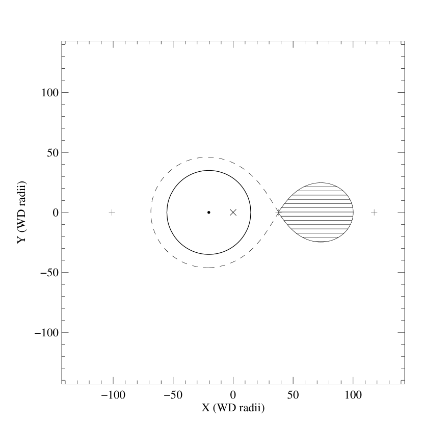
Figure 3: To-scale diagram of V592 Cas, including the model components (based on the parameters listed in Table 3 and discussed in the text). The diagram shows the secondary star (horizontal hatched area), WD (small filled circle), WD Roche lobe (dashed line), and the accretion disk (solid line around the WD marks the outer edge). The circumbinary dust disk, which has an inner radius of 700 $R_{\rm wd}$, is not shown. The inner and outer Lagrange points (plus symbols) and system center of mass (cross symbol) are also shown. The CV is depicted as viewed from “above” (i.e., with the orbital plane in the plane of the sky, equivalent to a system inclination of $0^{\circ}$).

Our custom-built IR SED modeling code for CVs is described in Brinkworth et al. (2007) and Hoard et al. (2007). We have continued to improve the code by implementing a model component to represent the accretion disk in non-magnetic CVs (described below). For this work, we have used a model consisting of a WD (denoted with subscript “wd”), secondary star (subscript “ss”), optically thick steady state accretion disk (subscript “acd”), and optically thin circumbinary dust disk (subscript “cbd”) to compare to the observed SED of V592 Cas. The system and model parameters are listed in Table 3, and Figure 2 (bottom) shows the SED data for V592 Cas with the nominal model. Figure 3 shows a to-scale diagram of V592 Cas based on the nominal model. We discuss some details of the model components and parameter choices below.

3.2.1 The White Dwarf

The WD is represented by a blackbody curve with $T_{\rm wd}=45,000$ K, which was chosen as a “typical” WD temperature for novalike CVs (e.g., Araujo-Betancor et al. 2003; Hoard et al. 2004). We have kept the WD temperature fixed at this value throughout our model calculations; for example, ignoring the possible role of the rate of mass accretion in heating the WD. In any case, as described below, even at this temperature the WD is only a minor contributor to the total system flux distribution longward of the ultraviolet (UV). If the temperature of the WD in V592 Cas is significantly different than this, then it is most likely to be smaller (Sion, 1999), which would make the WD even less significant in the determination of a model that can reproduce the long wavelength observations.

The WD is assumed to have the mean WD mass in CVs with $P_{\rm orb}<6$ hr, $M_{\rm wd}=0.75\,M_{\odot}$ (Knigge, 2006), and a corresponding radius of $R_{\rm wd}=0.0106\,R_{\odot}$ (Hamada & Salpeter, 1961; Panei et al., 2000). The projected surface area of the WD has been reduced by 7%, consistent with obscuration by an accretion disk (see below) that extends outward from $R_{\rm acd,in}=1R_{\rm wd}$ at the system inclination of $i=28^{\circ}$ (Huber et al., 1998).

3.2.2 The Secondary Star

The empirical CV secondary star sequences of Smith & Dhillon (1998) and Knigge (2006) predict a secondary star spectral type of M4.5$\pm$1 V (their Equation 4) and M4$\pm$2 V (his Figure 9), respectively, for the 2.76 hr orbital period of V592 Cas. That is, regardless of the true nature of the secondary stars in CVs, which likely differ in internal structure from corresponding single main sequence stars (e.g., by being oversized and/or slightly evolved as a result of their history of mass loss and irradiation – see discussion in Knigge 2006 and references therein) and/or by being non-uniformly heated by irradiation from the WD and accretion disk, the secondary star in V592 Cas has the spectroscopic appearance of a main sequence star with spectral type in the range indicated above. As it turns out (see Figure 2), the nominal secondary star contributes $\lesssim 2.5$% of the total flux density at all wavelengths, so the choice of secondary star template is robust against significant changes in spectral type or overall stellar temperature/luminosity that might be produced by evolutionary or irradiation effects (e.g., changing to an M2 template increases the maximum secondary star contribution to only $\sim 4$% of the total SED).

Thus, to represent the secondary star, we have used an empirical template of an M5.0 V star (GJ1093) constructed from optical (Mermilliod, 1986; Monet et al., 2003), 2MASS near-IR, and Spitzer IRAC (Patten et al., 2006) photometry. The secondary star template was extended to wavelengths longer than 8 $\mu$m by extrapolating the shorter wavelength data along a Rayleigh-Jeans tail (i.e., $f_{\nu}\propto\lambda^{-2}$). The secondary star template was scaled from the trigonometric parallax distance of $d=7.76$ pc for GJ1093 (Oppenheimer et al., 2001) to the adopted distance of V592 Cas, $d=360$ pc (see §3.1.1). Average mass, initial radius, and temperature values for a star of this spectral type (compiled in Cox 2000) were used in the model.

3.2.3 The Accretion Disk

The accretion disk component assumes an optically thick steady state disk composed of concentric rings emitting as blackbodies, following the “standard model” prescription in Frank, King, & Raine (2002). The accretion disk component is parameterized by inner and outer radii ($R_{\rm acd,in}$ and $R_{\rm acd,out}$), height at the inner radius ($h_{\rm acd}$), and a mass transfer rate from the secondary star ($\dot{M}$). The inclination of the disk is assumed to be the same as the system inclination; higher inclination systems have smaller projected surface area, resulting in an overall decrease in the effective brightness of the disk. In the case of V592 Cas, the inclination is quite low ($i=28^{\circ}$) so obscuration of the WD by the disk (and vice-versa), although included in our model calculation, has an insignificant effect on the resultant SED.

The general shape of the model accretion disk SED is similar to a slightly flattened and stretched blackbody function; that is, it displays a relatively broad peak with a rapid drop in brightness on the short wavelength side and a gradual (Rayleigh-Jeans-like) decline on the long wavelength side (e.g., see Figure 20 in Frank, King, & Raine 2002). In general, increasing either the disk area (i.e., making $R_{\rm acd,out}$ larger) or the mass transfer rate causes the overall accretion disk SED to become brighter. Increasing $R_{\rm acd,out}$ also tends to shift the peak of the accretion disk SED toward longer wavelengths, as more surface area is present in the cooler outer regions of the disk. Increasing $\dot{M}$ tends to shift the peak of the accretion disk SED toward shorter wavelengths, as the temperature in the inner disk increases.

Our accretion disk models for V592 Cas were composed of 100 concentric rings, each of which contains 1441 azimuthal sections (corresponding to 0.25^∘ per section). In addition, the outer edge of the accretion disk also contributes to the total disk SED. A wavelength- and temperature-dependent correction for limb darkening of the accretion disk is applied to each azimuthal section using linear limb darkening coefficients interpolated over the grid presented by Van Hamme (1993). In the case of a flat disk, this is a relatively simple procedure, as the disk face everywhere presents the same viewing angle (i.e., angle between the line-of-sight and a normal to the disk face), so only the disk edge is limb-darkened across a range of viewing angles. However, in the case of a flared disk (see below), which presents different viewing angles for different parts of the disk, limb darkening is calculated individually for each azimuthal section in each ring. The primary effect of limb darkening is to make the short wavelength end of the SED fainter relative to the long wavelength end.

By default, the standard model radial temperature profile from Frank, King, & Raine (2002) (their Equation 5.41) is used to determine the temperature in each disk ring. It is possible for the standard model radial temperature profile ($T\propto r^{-\gamma}$ with $\gamma=0.75$) to be modified by irradiation; that is, by reabsorption in the outer disk of flux from the central object and/or inner disk. Irradiation is primarily important in flared disks (i.e., disks whose height increases with radius), which can more easily intercept luminosity from the WD and inner disk. In order to account for this possibility, we have provided an option to utilize the irradiation prescription of Orosz & Wade (2003), in which the radial temperature profile of the outer accretion disk (at $R_{\rm acd}\geq R_{\rm crit}$, where $R_{\rm crit}=((7-8\gamma_{\rm out})/(6-8\gamma_{\rm out}))^{2}\,R_{\rm WD}$) is allowed to have a shallower temperature gradient than in the standard model ($\gamma_{\rm out}<0.75$). At the same time, the height of the disk for radii larger than $R_{\rm crit}$ is assumed to increase as $R^{9/8}$ (equation 2.51b in Warner 1995). The outer edge of the disk, which does not “see” the WD and inner disk, is always assumed to have a non-irradiated temperature appropriate for the standard model radial temperature profile.

As found in Orosz & Wade (2003) and other studies of the effect of irradiation on model accretion disk SEDs (e.g., Wade 1988), we found that irradiation (like limb darkening) primarily affects the short wavelength end of the SED. However, irradiation (which effectively raises the temperature at a given radius over the non-irradiated case) tends to make the short wavelength end of the SED brighter relative to the long wavelength end, which somewhat counteracts the effect of limb darkening. Changing (increasing) the mass transfer rate can often compensate for the combined effects of limb darkening and irradiation in the model accretion disk SED compared to the flat disk (i.e., no irradiation) case. However, for small values of $\gamma_{\rm out}$, the model SED becomes too faint at the short wavelength end, such that increasing $\dot{M}$ enough to supply the “missing” UV flux causes the accretion disk to exceed the observed SED at longer (e.g., IRAC bandpass) wavelengths. For V592 Cas, this occurs for $\gamma_{\rm out}\lesssim 0.60$, which requires $\dot{M}\gtrsim 1.8\times 10^{-8}\,M_{\odot}$ yr^-1 to reproduce the short wavelength end of the SED, but then exceeds (with the accretion disk component alone) the observed flux densities in the 2MASS and IRAC bands. Figure 2 shows SED models for V592 Cas using either a limb-darkened flat accretion disk or a limb-darkened flared accretion disk with irradiation ($\gamma_{\rm out}=0.7$). There is no significant difference in the resultant total model SEDs. The corresponding model parameters for each case are given in Table 3. In the remaining analysis, we utilize the flared accretion disk model.

It is not surprising that the accretion disk of a nearly face-on novalike CV is very bright. Indeed, the nominal accretion disk component for V592 Cas dominates at all wavelengths from the optical through near-IR, and even into the mid-IR (IRAC) range, accounting for all but $\lesssim 10$% of the total flux density in the wavelength range 0.5–5 $\mu$m. This makes accounting for the flux density that is in excess of the accretion disk model component at long wavelengths ($\lambda\gtrsim 8$ $\mu$m) the principle challenge to reproducing the observed SED of V592 Cas.

Figure 4 shows the effect of changing $R_{\rm acd,out}$ (top panel) or $\dot{M}$ (bottom panel) in the nominal flared accretion disk component. It is clear from this figure that adjusting either parameter individually can not account for the flux density excess at long wavelengths. In the case of $R_{\rm acd,out}$, the maximum allowed value is $\approx 45R_{\rm wd}$, corresponding to the size of the WD Roche lobe, and even this is insufficient to reproduce the 16- and 24-$\mu$m measurements. Increasing $\dot{M}$ also fails – when the model is bright enough to match the 16-$\mu$m measurement, then it is not bright enough to match at 24 $\mu$m, and when it would be bright enough to match the 24-$\mu$m measurement, then it would be too bright at 16 $\mu$m. The latter case would require an exceptionally high mass transfer rate, in excess of $10^{-6}\,M_{\odot}$ yr^-1, which is not plausible. Even worse, in order to match even the 16-$\mu$m measurement by increasing either parameter (even disregarding the firm upper limit to $R_{\rm acd,out}$), the model flux density greatly exceeds the observed values at shorter wavelengths. Changing both parameters in unison (e.g., increasing $R_{\rm acd,out}$ while decreasing $\dot{M}$) also does not produce a viable solution, since this does not change the slope of the long wavelength end of the accretion disk model component – it will never match both the 16- and 24-$\mu$m measurements at the same time, and will always be too bright at shorter wavelengths when it is forced to match either of the longer wavelength measurements. We are left with the conclusion that, in the context of the standard steady state accretion disk model (with or without irradiation), an additional component must be present to explain the observed 16- and 24-$\mu$m data – this is discussed in §3.2.4.

The nominal accretion disk outer radius is $R_{\rm acd,out}=35R_{\rm wd}$, which is equivalent to about 75% of the WD Roche lobe radius. This is consistent with estimates for the sizes of accretion disks in novalike CVs, which, at the mass ratio of V592 Cas, range from $\sim 0.3R_{\rm L1}$ from the theory for a zero viscosity disk to $\sim 0.4$–$0.8R_{\rm L1}$ from disk reconstructions based on eclipse observations (Ritter, 1980; Sulkanen et al., 1981; Rutten et al., 1992). The mass transfer rate, $\dot{M}\approx 1\times 10^{-8}\,M_{\odot}$ yr^-1 is in the middle of the $\sim 10^{-9}$–$10^{-8}\,M_{\odot}$ yr^-1 range that is often cited as characteristic of novalike CVs (Warner, 1995). Taylor et al. (1998) estimated a mass transfer rate of $9\times 10^{-9}\,M_{\odot}$ yr^-1 for V592 Cas from a power law fit to an optical–near-IR SED, which is quite close to our result (we note that if we utilize a flat standard model accretion disk with no irradiation and no limb darkening, then our best match to the observed SED is obtained with $\dot{M}=9\times 10^{-9}\,M_{\odot}$ yr^-1, as found by Taylor et al. 1998).

The orbital period of V592 Cas places it at the upper end, or well inside, the CV orbital period gap (depending on whose period limits for the gap are used; e.g., 2.1–2.8 hr, Patterson 1984; 2.10–2.85 hr, Howell et al. 2001, 2.19–2.75 hr, Shafter 1992; 2.15–3.18 hr, Knigge 2006; 2.25–2.75 hr, Politano & Weiler 2007; 2.3–2.8 hr, Warner 1995). From extrapolating between the expected mass transfer rates at either end of the period gap (e.g., Warner 1995; Howell et al. 2001), we would expect that at the orbital period of V592 Cas, in the absence of whatever mechanism causes the gap, it should have $\dot{M}\sim 10^{-9}\,M_{\odot}$ yr^-1, an order of magnitude smaller than inferred here and in Taylor et al. (1998). However, the observed spread in $\dot{M}$ at the long period end of the gap ranges from $\sim 10^{-10}$–$10^{-8}\,M_{\odot}$ yr^-1 (Patterson, 1984; Kolb et al., 2001). In any case, the mere fact that V592 Cas is a CV inside the period gap but still accreting at a high rate implies that it is not a run of the mill CV. It has either recently evolved into the gap and is in the process of shutting down mass transfer, or is a relatively young CV that only recently initiated mass transfer at close to its current orbital period.

3.2.4 The Circumbinary Dust Disk

In order to supply the requisite additional flux density at the longest mid-IR wavelengths, we utilize a circumbinary dust disk component. This model component is calculated as described in Hoard et al. (2007), under the assumption that the disk is optically thin, and composed of spherical grains with radius of 1 $\mu$m that (re)radiate as blackbodies. The problem of determining the inner boundary condition of temperature in the presence of multiple irradiating bodies (i.e., the WD, secondary star, and accretion disk), as described in Brinkworth et al. (2007), is also an issue for V592 Cas. Because the WD in V592 Cas is relatively hot, and both the secondary star and accretion disk are large, we expect that the maximum radius at which the dust temperature would be above 1000 K (i.e., in the 1000–2000 K range for dust sublimation) is on the order of 200–300 $R_{\rm wd}$ in V592 Cas. This is well beyond the tidal truncation limit of $\approx 1.5$ times the binary separation (about $157R_{\rm wd}$ for V592 Cas), which we have assumed for the inner edge radius of the circumbinary disk in previous works. Consequently, we have used the “equivalent star” prescription given in Brinkworth et al. (2007) to set the temperature at the inner edge of the circumbinary disk for a given radius. We note that essentially identical circumbinary disk SEDs can be obtained using different combinations of inner and outer radii by adjusting the total mass in the disk (e.g., we can obtain an SED identical to the one shown in Figure 2 by forcing the circumbinary disk inner edge radius to be at the tidal truncation radius, if the total mass of dust in the disk is increased by a factor of $\approx 5$). Similarly, the effect of different prescriptions for the radial temperature profile for the dust can be offset by adjusting the inner/outer radii and/or total mass of the circumbinary disk. In the context of reproducing the observed data, the important parameter is the temperature at the inner edge of the disk – it cannot be significantly higher than $\sim 500$ K, or the circumbinary disk component SED becomes too bright at short wavelengths to match the observations.

4 Discussion

4.1 Excluding Bremsstrahlung Emission

Howell et al. (2006) discuss several general reasons why bremsstrahlung, or free-free, emission in an outflowing wind can be excluded as a significant source of mid-IR emission in CVs. Dubus et al. (2004) present quantitative observational tests that would confirm or refute IR emission in CVs as being caused by bremsstrahlung emission. The first of these relates to the expected $f_{\nu}\propto\nu^{0.6}$ spectrum of bremsstrahlung emission. At 16 $\mu$m, the IR excess in V592 Cas (i.e., the remaining flux after the wd+ss+acd model components have been subtracted) is 0.33 mJy; at 24 $\mu$m, the excess is 0.30 mJy. This is a ratio of $f_{\nu,24}/f_{\nu,16}=0.91$, whereas if the IR excess followed a spectral law consistent with bremsstrahlung emission, then we should expect the flux density at 24 $\mu$m to be $\approx 0.78\times$ the flux density at 16 $\mu$m.

The second test relates to the wind mass loss rate required to explain the observed level of IR excess via bremsstrahlung emission. Using Equation 4 from Dubus et al. (2004) (which is based on the work of Wright & Barlow 1975) with an assumed wind velocity of 2000 km s^-1 (Kafka et al. 2008 found wind velocities reaching up to 5000 km s^-1 in V592 Cas), the observed IR excesses at 16 and 24 $\mu$m would require wind mass loss rates of $\approx 4.0$–$5.2\times 10^{-9}\,M_{\odot}$ yr^-1. This is equivalent to $\approx$25–35% of the entire inferred mass transfer rate from the secondary star in V592 Cas and, as such, is improbably high for the wind mass loss rate.

4.2 No Dust Emission at Short Wavelengths

Belle et al. (2004) concluded that there is no evidence for the presence of a circumbinary dust disk in the IR SED for V592 Cas; however, their data spanned only the $JHKL^{\prime}$ bands (i.e., $\approx 1.2$–$3.8$ $\mu$m). From our data, it is clear that the IR excess in V592 Cas is not readily apparent until well past 5 $\mu$m. For example, at wavelengths $\lesssim 5$ $\mu$m, the wd+ss+acd components account for $>90$% of the observed flux density, whereas at wavelengths $\gtrsim 8$ $\mu$m, these components account for $<70$% of the observed flux density. At $L^{\prime}$, only 3% of the observed flux density is not accounted for by the wd+ss+acd components. In addition, Belle et al. (2004) were looking for a much hotter circumbinary disk component, with $T\sim 3000$ K, whereas our observations show that the maximum temperature of the dust is $T\approx 500$ K. We want to emphasize that this is not just a case in which a bright, near-face-on accretion disk is “masking” fainter dust emission at short wavelengths. Dust at hotter temperatures in V592 Cas would have been detectable at $\lambda\lesssim 5$ $\mu$m, even against the comparatively bright contribution of the accretion disk at those wavelengths, if the long wavelength end of the dust distribution was bright enough to reproduce the observed 16- and 24-$\mu$m measurements.

4.3 Dissipation and Formation of the Dust

One question that has plagued a full understanding of the presence of circumbinary disks in CVs is the origin of the dust. Possible scenarios include: a remnant of the common envelope phase of the CV’s early evolution, formation through tidal disruption of minor planets or comets that survived from the progenitor solar system (as assumed for the origin of circumstellar dust disks around single WDs), creation via mass outflows in winds and nova outbursts from the inner binary (the mechanism assumed for the formation of circumbinary dust disks in the theoretical models of Willems et al. 2007), or some combination of these processes. Regardless of the exact origin of the dust, since the calculation of the structure of the circumbinary disk is predicated on the assumption that there is a region in the CV system in which temperatures are too high for dust to exist, it seems likely that the circumbinary disks cannot be entirely static: dust will be sublimated at some rate at the inner edge as grains stray too close to the inner binary, and another trickle of dust will be lost at the outer edge of the circumbinary disk as grains stray too far away from the gravitational influence of the inner binary. So, it might be more appropriate to wonder about not only the origin of the dust, but its longevity as well. In V592 Cas, at least, there is an obvious mechanism to provide a continuing supply of raw materials for the circumbinary disk, namely, the wind outflow discussed in Witherick et al. (2003), Prinja et al. (2004), and Kafka et al. (2008).

The total circumbinary dust disk mass in V592 Cas amounts to only $\sim 10^{-12}\,M_{\odot}$, which is a small fraction ($\sim 0.01$%) of the total annual mass transfer budget in this system. If the total mass flux present in the wind outflow from V592 Cas is a tenth of a percent of the total mass transfer budget, and even if the efficiency of capturing material from the wind into the circumbinary disk is a similarly small fraction, then this mechanism can still completely replenish the circumbinary disk on a timescale of $\sim 100$ yr. Another way to look at this is that as long as the mass loss rate from the circumbinary disk (e.g., dissipation through sublimation and/or escape from the system) is smaller than the rate of dust formation from the wind, then the wind can maintain the circumbinary disk at a constant mass. Using the 0.1% efficiencies for the wind outflow and dust formation rates, as suggested above, the circumbinary disk mass will be maintained as long as $\lesssim 1$% of the total circumbinary disk mass is lost per year. This result also implies that in V592 Cas a much more massive circumbinary disk probably could not be maintained by the wind outflow alone.

4.4 Total Mass of Circumbinary Dust

The total mass in our model circumbinary dust disk is $M_{\rm cbd}\approx 10^{21}$ g. Reasonable variations in the inner radius of the circumbinary disk that would be required to yield the necessary boundary condition of $T_{\rm cbd,in}\approx 500$ K in the presence of different irradiation prescriptions (i.e., treatment of multiple heating sources in the inner binary) can be balanced against changing the total mass in the circumbinary dust disk to produce an SED that is indistinguishable from the one presented here. In addition, the photometric uncertainties also provide some leeway for changing the dust mass while still adequately reproducing the observed SED. However, these variations in mass are relatively small (i.e., factor of $\lesssim 5$). The mass of the circumbinary disk in V592 Cas exceeds those found in several of our past investigations of short orbital period magnetic CVs, which were on the order of $10^{15}$–$10^{17}$ g (Brinkworth et al., 2007). It is comparable to the high end of the range of mass estimates for the circumbinary disk in the short orbital period, magnetic CV EF Eri (Hoard et al., 2007). However, as found in all of these previous studies, the total mass of dust is many orders of magnitude smaller than the $10^{28}$–$10^{29}$ g predicted to be necessary for circumbinary disks to serve as angular momentum loss mechanisms that can significantly affect the secular evolution of CVs (Taam et al., 2003; Willems et al., 2007). The prediction by Willems et al. (2007) that the circumbinary dust disks in (disk-accreting) CVs should only be detectable at wavelengths longer than 10 $\mu$m is borne out by our observations for the case of V592 Cas.

The outer radius of the circumbinary disk has been somewhat arbitrarily set at 15,000 $R_{\rm wd}$, giving an outer temperature of 50 K, comparable to what one might expect as the disk merges with the local ISM. The model SED at the observed wavelengths is not sensitive to decreasing this outer radius by more than a factor of 2, corresponding to an outer temperature of $\sim 100$ K. However, in order to continue to match the observed mid-IR photometry, the total mass of dust in the disk must be decreased as the outer radius decreases – this exacerbates the low mass discrepancy of the circumbinary disks compared to the expectation from CV evolution theory. Unfortunately, applying the reverse of this scenario also cannot resolve the low mass problem: increasing the outer radius of the circumbinary disk to as much as 100,000 $R_{\rm wd}$ (corresponding to a rather low temperature of only 12 K) only increases the requisite total dust mass by a factor of $\sim 7$.

4.5 Excluding an Optically Thick Circumbinary Disk

The evolutionary calculations of Taam et al. (2003) and Willems et al. (2007) assume that the circumbinary disks are massive ($\gtrsim 10^{28}$ g), hot ($T_{\rm cbd,in}\approx 1500$–$3000$ K), and optically thick. If the circumbinary disks in CVs do not have these characteristics, then we should not expect them to act as effective angular momentum loss mechanisms during the course of CV evolution. Brinkworth et al. (2007) and Hoard et al. (2007) discussed the reasons for preferring an optically thin circumbinary disk model over an optically thick one when attempting to match the observed IR excesses of magnetic CVs. For the sake of completeness, and because it would offer the simplest method for substantially increasing the dust mass in V592 Cas compared to the optically thin case, we have also explored the optically thick circumbinary disk case. We can produce a model circumbinary disk SED very similar to that shown in Figure 2 using an optically thick treatment. However, we must force the circumbinary disk to have an inner edge temperature of $T_{\rm cbd,in}\approx 500$ K at the tidal truncation radius – this is a factor of $\approx 3$–4 cooler than the expected temperature at this radius due to irradiation from the WD. Starting the circumbinary disk at a larger radius where the expected temperature is closer to $\approx 500$ K does not work because the correspondingly larger surface area of the circumbinary disk makes the SED component too bright to match the observed mid-IR data. In addition, the circumbinary disk must be truncated at an outer radius corresponding to a temperature of $\approx 250$ K, much warmer than the ambient temperature of the ISM, or the model SED component is too bright at the long wavelength end of the observed range. These inconsistencies again suggest that the optically thick case is not appropriate for matching the shape of the observed IR excess in V592 Cas. Thus, we are led to conclude that the results from the optically thin case are more likely to be representative of the distribution of dust.

4.6 An Initially Massive Circumbinary Disk?

Considering the low dust masses that we have found in several CVs (now including a high $\dot{M}$ novalike CV with a wind; that is, a good candidate to have a large amount of circumbinary material), we wonder if an initially massive circumbinary disk (perhaps formed during the common envelope phase of the CV’s early history) could evolve over time into a low mass remnant that we see now. To begin to address this question, we have used a “toy” model to explore the general behavior of an initially massive circumbinary dust disk in the presence of dissipation at the disk edges and contribution from formation of new dust using material in the wind from the inner binary, as described in §4.3. This model is purely parametric, and does not consider the precise physics of how a particular rate of dust dissipation or formation might arise. The total mass of circumbinary dust as a function of time (years) is simply calculated under the assumption that a constant small fraction ($\varepsilon_{1}$) of the total dust mass is lost each year through dissipation. At the same time, a small fraction ($\varepsilon_{2}$) of the mass transfer rate in the CV ($\dot{M}$) is carried away in a wind, of which another small fraction ($\varepsilon_{3}$) forms dust and contributes to the mass of the circumbinary disk. That is,

$$M_{\rm cbd,i}=(1-\varepsilon_{1})M_{\rm cbd,i-1}+\varepsilon_{2}\varepsilon_{3}\dot{M},$$ (1)

and this equation is evaluated over $i=1$–$10^{8}$ yr, with initial mass of at least $10^{28}$ g at $i=0$. We assume that $\log(\dot{M})\propto-\log(i)$ (i.e., the mass transfer rate decreases linearly in log-log space), with an initial value of $\dot{M}_{\rm initial}=10^{-7.5}\,M_{\odot}$ yr^-1, and evolve the system over $10^{8}$ yr to a final mass transfer rate of $10^{-8}\,M_{\odot}$ yr^-1 or smaller. This evolving mass transfer rate, to first order, mimics the expected decrease in $\dot{M}$ during the evolution of a CV above the period gap (e.g., Shafter 1992; Warner 1995; Howell et al. 2001).

Several examples of the outcome of this calculation are shown in Figure 5. In general, the dust mass follows a similar evolution in all cases, over a wide range of values for $\dot{M}_{\rm final}$, $M_{\rm cbd,i=0}$, $\varepsilon_{1}$, $\varepsilon_{2}$, and $\varepsilon_{3}$. It first goes through a period of nearly exponential decline during which the rate of mass contributed to the circumbinary dust as new dust forms is insignificantly small compared to the total mass of dust, and the losses from the circumbinary dust (parameterized by $\varepsilon_{1}$) dominate. At some critical time, $\tau_{\rm crit}$ (marked by a sharp “elbow” in the plot of $\log({\rm time})$ vs. $\log({\rm dust\,mass})$), the rate of mass being contributed to the circumbinary dust by the wind (parameterized by $\varepsilon_{2}$ and $\varepsilon_{3}$) becomes comparable to the rate of mass being lost, and the total dust mass becomes relatively stable for the remaining evolution of the system (showing at most only a gradual decline by less than an order of magnitude over many tens of millions of years). In general, the value of $\tau_{\rm crit}$ and the final dust mass both increase as $\varepsilon_{1}$ is decreased because mass is lost from the dust at a lower rate and, consequently, it takes longer for the contribution from the wind to become significant in comparison to the rate of dust dissipation and the total mass of dust. The value of $\tau_{\rm crit}$ also increases, to a lesser extent, when the initial dust mass is larger, because there is more dust to dissipate before the contribution from the wind becomes significant; however, if all other parameters are fixed, the evolution of the dust mass after $\tau_{\rm crit}$ is identical regardless of the value of $M_{\rm cbd,i=0}$.

Because $\varepsilon_{2}$ and $\varepsilon_{3}$ are used as a product in Equation 1, it does not matter for the sake of calculation which parameter is changed; however, they do have different physical interpretations, as defined above. Changing the product of $\varepsilon_{2}$ and $\varepsilon_{3}$ has only a small effect on $\tau_{\rm crit}$ for a given $\varepsilon_{1}$. This mainly affects the final total mass of dust, with the mass increasing as the product $\varepsilon_{2}\varepsilon_{3}$ increases, which causes the rate of dust formation out of the CV wind to increase and, consequently, become significant earlier compared to the total dust mass and rate of dust dissipation.

Panel (a) in Figure 5 shows the result of varying the circumbinary dust dissipation rate efficiency, $\varepsilon_{1}=0.01,0.001,0.0001$, with the wind-fueled dust formation rate efficiencies fixed at $\varepsilon_{2}=\varepsilon_{3}=0.001$. The result of this is to cause $\tau_{\rm crit}$ to vary from $\sim 10^{3}$–$10^{5}$ yr and the final dust mass to vary from $\sim 2\times 10^{20}$–$2\times 10^{22}$ g as $\varepsilon_{1}$ decreases. By comparison with the other cases (discussed below), it is clear that the value of $\varepsilon_{1}$ has the largest effect on $\tau_{\rm crit}$.

Panel (b) in Figure 5 shows the result of varying the product of the wind-fueled dust formation rate efficiencies, $\varepsilon_{2}\varepsilon_{3}=0.0001,0.00001,0.000001$, with the circumbinary dust dissipation rate efficiency fixed at $\varepsilon_{1}=0.001$. In this scenario, the value of $\tau_{\rm crit}$ is relatively unchanged at $\sim 10^{4}$ yr, but the final dust mass varies from $\sim 2\times 10^{20}$–$2\times 10^{22}$ g as $\varepsilon_{2}\varepsilon_{3}$ increases. In both panels (a) and (b) the initial dust mass and final mass transfer rate were fixed at $M_{\rm cbd,i=0}=10^{28}$ g and $\dot{M}_{\rm final}=10^{-9}\,M_{\odot}$ yr^-1, respectively.

Panel (c) in Figure 5 shows the result of varying the final mass transfer rate, $\dot{M}_{\rm final}=10^{-8},10^{-9},10^{-10}\,M_{\odot}$ yr^-1, with the dust dissipation and formation efficiences fixed at $\varepsilon_{1}=\varepsilon_{2}=\varepsilon_{3}=0.001$. For the dust mass evolution up to $\tau_{\rm crit}$, the result is very similar to the case shown in panel (b). After $\tau_{\rm crit}$, the total dust mass declines more slowly for larger values of $\dot{M}_{\rm final}$, since there is a correspondingly larger wind outflow from which new dust can form. The case for $\dot{M}_{\rm final}=10^{-8}\,M_{\odot}$ yr^-1 corresponds approximately to V592 Cas at the current time, and shows the least change in total dust mass in the post-$\tau_{\rm crit}$ evolution of the CV. The case for $\dot{M}_{\rm final}=10^{-9}\,M_{\odot}$ yr^-1 might be considered more “typical” of CVs at this orbital period, or could also represent the future of V592 Cas after continued evolution further reduces its mass transfer rate.

Finally, panel (d) in Figure 5 shows the result of changing the initial dust mass, $M_{\rm cbd,i=0}=10^{28},10^{30},10^{34}$ g, with the dust dissipation and formation efficiences fixed at $\varepsilon_{1}=\varepsilon_{2}=\varepsilon_{3}=0.001$ and the final mass transfer rate fixed at $\dot{M}_{\rm final}=10^{-9}\,M_{\odot}$ yr^-1. We had initially chosen $10^{28}$ g of dust as a lower limit starting point of interest; obviously, the case in which the initial mass of dust is already smaller than predicted to be necessary to affect CV evolution is of little interest. However, if the initial dust originates, for example, during the common envelope phase, then there could potentially be more than this lower limit case. However, as panel (d) shows, even an initial mass as much as $10^{6}$ times larger than the lower limit results in identical post-$\tau_{\rm crit}$ conditions and evolution, with only a small increase in $\tau_{\rm crit}$ as $M_{\rm cbd,i=0}$ increases.

In general, we find that this simple toy model suggests that even an initially very massive ($>>10^{28}$ g) circumbinary dust disk present at the birth of a CV will rapidly evolve (in only $10^{3}$–$10^{5}$ yr) into a disk with much lower mass ($\sim 10^{20}$–$10^{22}$ g). The dust disk mass is then approximately stable over the remaining evolution of the CV. The only requirements to produce this scenario are that the circumbinary dust experiences ongoing low rates of dissipation (e.g., via sublimation and escape from the system’s gravity) and formation (e.g., from material carried outward in a wind from the inner binary). If a massive circumbinary dust disk is a common by-product of the common envelope phase of CV formation, then such a scenario might explain why all of the CVs so far observed with Spitzer appear to have only small amounts of circumbinary dust. We are encouraged by the relatively close agreement between our inferred mass of dust in V592 Cas and the toy model prediction for the final mass of circumbinary dust in a high mass transfer rate CV that has evolved to the long period end of the period gap.

To first order, the initial rapid decrease in the mass of circumbinary dust would seem to imply that circumbinary dust disks do not play a role in the secular evolution of the CV population. However, this begs a new question: is the presence of a massive circumbinary disk for a short time early in the evolutionary history of a CV sufficient to have a lasting impact on the secular evolution of the CV? That is, could such a scenario result in an early episode of extra angular momentum loss of sufficient magnitude to alter the characteristics at the far end of the evolutionary sequence of the CV population compared to predictions utilizing angular momentum loss via magnetic braking and gravitational radiation alone? The answer to that question is beyond the scope of this paper.

5 Conclusions

We have found compelling observational evidence for the existence of IR excess in the near-face-on, novalike CV V592 Cas. This result stems primarily from our new Spitzer IRS-PUI and MIPS observations at 16 and 24 $\mu$m, respectively. We have provided a representative model that reproduces the observed (dereddened) SED using a combination of white dwarf, secondary star, steady state accretion disk, and circumbinary dust disk components. At short wavelengths ($\lambda\lesssim 5$ $\mu$m), the SED of V592 Cas is dominated by the steady state accretion disk and, as found in past studies of this system, there is no indication of the presence of circumbinary material until the SED at longer wavelengths is considered. The total mass in the circumbinary dust disk of V592 Cas, consistent with recent studies of IR excess in magnetic CVs, is apparently too small to have a significant effect on the secular evolution of the CV. This is the first estimate for the mass of circumbinary dust in a non-magnetic, disk-accreting CV at an orbital period ($\approx 166$ min) significantly longer than the observed period minimum ($\approx 80$ min), and demonstrates that the low dust mass results from our previously studied systems are not solely a result of the fact that they contain strongly magnetic WDs.

The problem of accounting for the origin and/or longevity of the circumbinary dust is mitigated in the case of V592 Cas by the presence of a wind outflow, which can easily provide the necessary raw materials to replenish the circumbinary disk on short timescales or maintain it at a relatively constant mass. An implication of this result is that CVs without significant wind outflows might be expected to contain little or no circumbinary dust. However, our previous Spitzer observations of magnetic CVs show that dust can be present even in systems that lack a strong wind. So, there must be more than one route to the presence of circumbinary dust in CVs.

We have made a simple calculation that shows that an initially massive circumbinary dust disk, perhaps formed during the common envelope phase of the binary’s early evolution, will rapidly evolve to a relatively stable low mass in the presence of ongoing low rates of dissipation of dust in the existing circumbinary material and formation of new dust (for example, fueled by matter carried outward in a wind from the inner binary). It remains to be demonstrated in detail whether or not such evolving circumbinary disks can still play a role in the secular evolution of the CV population.

Table 1: Spectral energy distribution data

		Flux Density:
Band	Wavelength	Observed	Dereddened	Date Obtained
	(microns)	(mJy)	(mJy)	(UT)
UV	$0.1450$	$19.99\pm 2.00$	$120\pm 25$	05 Dec 1981
UV	$0.1800$	$20.53\pm 2.05$	$105\pm 19$	05 Dec 1981
V	$0.55\pm 0.045$	$36.11^{+3.36}_{-3.65}$	$66.6\pm 7.0$	08 Oct 2005
2MASS-J	$1.235^{+0.125}_{-0.115}$	$19.27\pm 0.53$	$22.28\pm 1.85$	28 Sep 2000
2MASS-H	$1.662^{+0.118}_{-0.152}$	$12.82^{+0.44}_{-0.45}$	$13.95\pm 1.32$	28 Sep 2000
2MASS-Ks	$2.159^{+0.141}_{-0.139}$	$8.88\pm 0.25$	$9.35\pm 0.91$	28 Sep 2000
IRAC-1	$3.550\pm 0.375$	$4.15\pm 0.19$	$\cdots$	18 Aug 2005
IRAC-2	$4.493\pm 0.508$	$2.92\pm 0.14$	$\cdots$	18 Aug 2005
IRAC-3	$5.731\pm 0.713$	$1.98\pm 0.12$	$\cdots$	18 Aug 2005
IRAC-4	$7.872\pm 1.453$	$1.22\pm 0.10$	$\cdots$	18 Aug 2005
IRS-PUI-blue	$15.8^{+2.9}_{-2.5}$	$0.56\pm 0.08$	$\cdots$	16 Jan 2006
MIPS-24	$23.675^{+2.425}_{-2.875}$	$0.43\pm 0.07$	$\cdots$	21 Feb 2006

Table 2: Photometry of V592 Cas

JD	Year	$U$	$B$	$V$	$R$	$J$	$H$	$K_{\rm s}$	Reference
c. 2438761	c. 1965	12.07:	12.86:	12.79:	$\cdots$	$\cdots$	$\cdots$	$\cdots$	Haug (1970)
2449394.20–2449401.28	1993.112–1994.131	$\cdots$	12.5–12.7	$\cdots$	$\cdots$	$\cdots$	$\cdots$	$\cdots$	Taylor et al. (1998)
2450302.68–2450303.72	1996.600–1996.603	$\cdots$	$\cdots$	12.8(1)	$\cdots$	$\cdots$	$\cdots$	$\cdots$	Huber et al. (1998)
2450357.84	1996.751	$\cdots$	$\cdots$	$\cdots$	$\cdots$	12.8(2)	12.2(2)	12.3(2)	Huber et al. (1998)
2450741.64–2450836.62	1997.803–1998.063	$\cdots$	$\cdots$	12.7(1)	$\cdots$	$\cdots$	$\cdots$	$\cdots$	Taylor et al. (1998)
2451815.92	2000.742	$\cdots$	$\cdots$	$\cdots$	$\cdots$	12.294(23)	12.256(31)	12.189(23)	2MASS
2452568.53–2452568.67	2002.805	$\cdots$	$\cdots$	$\cdots$	12.16–12.46	$\cdots$	$\cdots$	$\cdots$	Kato & Starkey (2002)
2453651.87–2453651.95	2005.770	$\cdots$	$\cdots$	12.55(10)	$\cdots$	$\cdots$	$\cdots$	$\cdots$	Kafka et al. (2008)
2453742.68–2454450.62	2006.019–2007.959	$\cdots$	$\cdots$	$\cdots$	12.3(3)	$\cdots$	$\cdots$	$\cdots$	AAVSO

Table 3: Model component parameters

Component	Parameter	Value	Source
System:	Inclination, $i$ (∘)	$28^{+11}_{-10}$	Huber et al. (1998)
	Orbital Period, $P_{\rm orb}$ (d)	0.115063(1)	Taylor et al. (1998)
	Distance, $d$ (pc)	364	Taylor et al. (1998), this work
WD:	Temperature, $T_{\rm wd}$ (K)	45,000	this work
	Mass, $M_{\rm wd}$ ($M_{\odot}$)	0.75	this work
	Radius, $R_{\rm wd}$ ($R_{\odot}$)	$0.0106$	this work
SS:	Spectral Type	M5.0	Smith & Dhillon (1998); Knigge (2006)
	Temperature, $T_{2}$ (K)	3030	Cox (2000)
	Mass, $M_{2}$ ($M_{\odot}$)	0.21	Cox (2000)
ACD:	Inner Radius, $R_{\rm acd,in}$ ($R_{\rm wd}$)	1.0, 1.0	this work
	Outer Radius, $R_{\rm acd,out}$ ($R_{\rm wd}$)	35.0, 35.0	this work
	Critical Radius, $R_{\rm crit}$ ($R_{\rm wd}$)	n/a, 12.25	this work
	Inner Height, $h_{\rm acd}$ ($R_{\rm wd}$)	0.1, 0.1	this work
	Outer Height, $h_{\rm acd}$ ($R_{\rm wd}$)	0.1, 3.36	this work
	Inner Temperature Profile Exponent, $\gamma$	0.75, 0.75	this work
	Outer Temperature Profile Exponent, $\gamma_{\rm out}$	n/a, 0.70	this work
	Mass Transfer Rate, $\dot{M}$ ($M_{\odot}$ yr-1)	$1.1\times 10^{-8}$, $1.5\times 10^{-8}$	this work
CBD:	Optical Depth Prescription	thin	this work
	Temperature Profile Exponent	0.75	this work
	Constant Height, $h_{\rm cbd}$ ($R_{\rm wd}$)	0.01	this work
	Grain Density, $\rho_{\rm grain}$ (g cm-3)	3.0	this work
	Grain Radius, $r_{\rm grain}$ ($\mu$m)	1	this work
	Inner Radius, $R_{\rm cbd,in}$ ($R_{\rm wd}$)	700	this work
	Outer Radius, $R_{\rm cbd,out}$ ($R_{\rm wd}$)	15,000	this work
	Inner Temperature, $T_{\rm cbd,in}$ (K)	500	this work
	Outer Temperature, $T_{\rm cbd,in}$ (K)	50	this work
	Total Mass, $M_{\rm cbd}$ (g)	$2.3\times 10^{21}$	this work

Note. — WD = white dwarf, SS = secondary star, ACD = accretion disk, CBD = circumbinary disk. Two values are listed for each of the ACD parameters, corresponding to the two models shown in Figure 2; all other parameters are the same for both models.

Figure 1: Per cent uncertainty (standard deviation) of measured IRAC flux densities as a function of average source flux density. The panels show (a) channel 1 (3.6 $\mu$m), (b) channel 2 (4.5 $\mu$m), (c) channel 3 (5.8 $\mu$m), and (d) channel 4 (8.0 $\mu$m). The solid vertical line in each panel is the mean flux density of V592 Cas in the corresponding channel. The vertical dashed lines show the $\pm 20$% range over which uncertainty measurements were averaged to arrive at the scatter term uncertainties for V592 Cas (large diamonds). See §2.1.1 for details.

Figure 2: Dereddened spectral energy distribution (top panel) and model (middle and bottom panels) for V592 Cas. The photometric data (see §3.1) are shown as filled circles. The system model (solid line) is composed of a WD (dotted line), M5.0 secondary star (short dashed line), steady state accretion disk (long dashed line), and circumbinary dust disk (dot-dot-dot dash line). The model in the middle panel utilizes a limb darkened flat accretion disk with no irradiation, while the model in the bottom panel utilizes a limb-darkened flared accretion disk with irradiation. See §3.2 for a discussion of the model parameters.

Figure 4: As in Figure 2, but showing a model that does not contain a circumbinary dust disk, in which a steady state accretion disk is the dominant component at all wavelengths. For clarity, only the total system model is plotted; the WD and secondary star are as shown in Figure 2. The top panel shows the effect of changing the outer radius of the accretion disk; from bottom to top the model curves have $R_{\rm acd,out}=5,15,25,35,45R_{\rm wd}$ (the nominal value is $35R_{\rm wd}$). The bottom panel shows the effect of changing the mass transfer rate through the accretion disk; from bottom to top, the model curves have $\dot{M}=0.01,0.1,1,10,100$ times the nominal value of $1.5\times 10^{-8}\,M_{\odot}$ yr^-1. All other model parameters are as given in Table 3.

Figure 5: Evolution of circumbinary dust mass as calculated using the toy model described in §4.6. In panels (a), (b), and (d), the CV’s mass transfer rate evolves from $10^{-7.5}\,M_{\odot}$ yr^-1 to $10^{-9}\,M_{\odot}$ yr^-1 over $10^{8}$ yr. Panel (a) shows the effect of changing the dust dissipation efficiency, $\varepsilon_{1}$, with values of 0.01, 0.001, and 0.0001 (curves from bottom to top, respectively) while keeping the dust contribution efficiencies fixed at $\varepsilon_{2}=\varepsilon_{3}=0.001$. Panel (b) shows the effect of changing the product of the dust formation efficiencies, $\varepsilon_{2}\varepsilon_{3}$, with values of 0.0001, 0.00001, and 0.000001 (curves from top to bottom, respectively) while keeping the dust dissipation efficiency fixed at $\varepsilon_{1}=0.001$. In panels (c) and (d) the dust dissipation and formation efficiencies were fixed at $\varepsilon_{1}=\varepsilon{2}=\varepsilon{3}=0.001$. Panel (c) shows the effect of changing the final mass transfer rate, with values of $10^{-8}$, $10^{-9}$, and $10^{-10}\,M_{\odot}$ yr^-1 (curves from top to bottom). Panel (d) shows the effect of changing the initial mass of circumbinary dust, with values of $10^{28}$, $10^{30}$, and $10^{34}$ g (curves from bottom to top). Note the different vertical axis scale in panel (d).

References

- Araujo-Betancor et al. (2003) Araujo-Betancor, S., et al. 2003, ApJ, 583, 437
- Belle et al. (2004) Belle, K. E., Sanghi, N., Howell, S. B., Holberg, J. B., & Williams, P. T. 2004, AJ, 128, 448
- Brinkworth et al. (2007) Brinkworth, C. S., et al. 2007, ApJ, 659, 1541
- Cardelli et al. (1989) Cardelli, J. A., Clayton, G. C., & Mathis, J. S. 1989, ApJ, 345, 245
- Ciardi et al. (1998) Ciardi, D. R., Howell, S. B., Hauschildt, P. H., & Allard, F. 1998, ApJ, 504, 450
- Cohen et al. (2003) Cohen, M., Wheaton, W. A., & Megeath, S. T. 2003, AJ, 126, 1090
- Cox (2000) Cox, A. N. 2000, in Allen’s Astrophysical Quantities, 4th ed. (New York: Springer-Verlag)
- Davis et al. (2000) Davis, J., Tango, W. J., & Booth, A. J. 2000, MNRAS, 318, 387
- Downes et al. (1995) Downes, R., Hoard, D. W., Szkody, P., & Wachter, S. 1995, AJ, 110, 1824
- Dubus et al. (2004) Dubus, G., Campbell, R., Kern, B., Taam, R. E., & Spruit, H. C. 2004, MNRAS, 349, 869
- Fazio et al. (2004) Fazio, G. G., et al. 2004, ApJS, 154, 10
- Fitzpatrick & Massa (2007) Fitzpatrick, E. L., & Massa, D. 2007, ApJ, 663, 320
- Frank, King, & Raine (2002) Frank, J., King, A., & Raine, D. 2002, in Accretion Power in Astrophysics (Cambridge: Cambridge University Press), ch. 5
- Greenstein et al. (1970) Greenstein, J. L., Sargent, A. I., & Haug, U. 1970, A&A, 7, 1
- Guinan & Sion (1982) Guinan, E. F., & Sion, E. M. 1982, Advances in Ultraviolet Astronomy, 465
- Hamada & Salpeter (1961) Hamada, T., & Salpeter, E. E. 1961, ApJ, 134, 683
- Harrison et al. (2004) Harrison, T. E., Johnson, J. J., McArthur, B. E., Benedict, G. F., Szkody, P., Howell, S. B., & Gelino, D. M. 2004, AJ, 127, 460
- Haug (1970) Haug, U. 1970, A&AS, 1, 35
- Henden & Honeycutt (1997) Henden, A. A., & Honeycutt, R. K. 1995, PASP, 107, 324
- Hoard et al. (2007) Hoard, D. W., Howell, S. B., Brinkworth, C. S., Ciardi, D. R., & Wachter, S. 2007, ApJ, 671, 734
- Hoard et al. (2004) Hoard, D. W., Linnell, A. P., Szkody, P., Fried, R. E., Sion, E. M., Hubeny, I., & Wolfe, M. A. 2004, ApJ, 604, 346
- Houck et al. (2004) Houck, J. R., et al. 2004, ApJS, 154, 18
- Howell et al. (2008) Howell, S. B., Hoard, D. W., Brinkworth, C. S., Kafka, S., Walentosky, M., Walter, F., & Rector, T. 2008, ApJ, 685, 418
- Howell et al. (2006) Howell, S. B., et al. 2006, ApJ, 646, L65
- Howell et al. (2001) Howell, S. B., Nelson, L. A., & Rappaport, S. 2001, ApJ, 550, 897
- Huber et al. (1998) Huber, M. E., Howell, S. B., Ciardi, D. R., & Fried, R. 1998, PASP, 110, 784
- Kafka et al. (2008) Kafka, S., Hoard, D. W., & Honeycutt, R. K. 2008, ApJ, submitted
- Kato & Starkey (2002) Kato, T., & Starkey, D. R. 2002, IBVS, 5358, 1
- Knigge (2006) Knigge, C. 2006, MNRAS, 373, 484
- Kolb et al. (2001) Kolb, U., Rappaport, S., Schenker, K., & Howell, S. 2001, ApJ, 563, 958
- Mermilliod (1986) Mermilliod, J.-C. 1986, Catalogue of Eggen’s UBV data, 0 (1986), 0
- Monet et al. (2003) Monet, D. G., et al. 2003, AJ, 125, 984
- Nandy et al. (1975) Nandy, K., Thompson, G. I., Jamar, C., Monfils, A., & Wilson, R. 1975, A&A, 44, 195
- Oppenheimer et al. (2001) Oppenheimer, B. R., Golimowski, D. A., Kulkarni, S. R., Matthews, K., Nakajima, T., Creech-Eakman, M., & Durrance, S. T. 2001, AJ, 121, 2189
- Orosz & Wade (2003) Orosz, J. A., & Wade, R. A. 2003, ApJ, 593, 1032
- Panei et al. (2000) Panei, J. A., Althaus, L. G., & Benvenuto, O. G. 2000, A&A, 353, 970
- Patten et al. (2006) Patten, B. M., et al. 2006, ApJ, 651, 502
- Patterson (1984) Patterson, J. 1984, ApJS, 54, 443
- Patterson (1998) Patterson, J. 1998, PASP, 110, 1132
- Politano & Weiler (2007) Politano, M., & Weiler, K. P. 2007, ApJ, 665, 663
- Prinja et al. (2004) Prinja, R. K., Knigge, C., Witherick, D. K., Long, K. S., & Brammer, G. 2004, MNRAS, 355, 137
- Rieke et al. (2004) Rieke, G. H., et al. 2004, ApJS, 154, 25
- Ritter (1980) Ritter, H. 1980, A&A, 91, 161
- Rutten et al. (1992) Rutten, R. G. M., van Paradijs, J., & Tinbergen, J. 1992, A&A, 260, 213
- Shafter (1992) Shafter, A. W. 1992, ApJ, 394, 268
- Sion (1999) Sion, E. M. 1999, PASP, 111, 532
- Smith & Dhillon (1998) Smith, D. A., & Dhillon, V. S. 1998, MNRAS, 301, 767
- Spruit & Taam (2001) Spruit, H. C., & Taam, R. E. 2001, ApJ, 548, 900
- Sulkanen et al. (1981) Sulkanen, M. E., Brasure, L. W., & Patterson, J. 1981, ApJ, 244, 579
- Taam et al. (2003) Taam, R. E., Sandquist, E. L., & Dubus, G. 2003, ApJ, 592, 1124
- Taylor et al. (1998) Taylor, C. J., et al. 1998, PASP, 110, 1148
- Van Hamme (1993) Van Hamme, W. 1993, AJ, 106, 2096
- von Braun et al. (2008) von Braun, K., van Belle, G. T., Ciardi, D. R., López-Morales, M., Hoard, D. W., & Wachter, S. 2008, ApJ, 677, 545
- Wade (1988) Wade, R. A. 1988, ApJ, 335, 394
- Warner et al. (1971) Warner, B., Robinson, E. L., & Nather, R. E. 1971, MNRAS, 154, 455
- Warner (1987) Warner, B. 1987, MNRAS, 227, 23
- Warner (1995) Warner, B. 1995, in Cataclysmic Variable Stars (Cambridge: Cambridge University Press)
- Werner et al. (2004) Werner, M. W., et al. 2004, ApJS, 154, 1
- Willems et al. (2005) Willems, B., Kolb, U., Sandquist, E. L., Taam, R. E., & Dubus, G. 2005, ApJ, 635, 1263
- Willems et al. (2007) Willems, B., Taam, R. E., Kolb, U., Dubus, G., & Sandquist, E. L. 2007, ApJ, 657, 465
- Witherick et al. (2003) Witherick, D. K., Prinja, R. K., Howell, S. B., & Wagner, R. M. 2003, MNRAS, 346, 861
- Wright & Barlow (1975) Wright, A. E., & Barlow, M. J. 1975, MNRAS, 170, 41
- Zwitter & Munari (1994) Zwitter, T., & Munari, U. 1994, A&AS, 107, 503