Accurate estimators of power spectra in $N$-body simulations

Abstract

A method to rapidly estimate the Fourier power spectrum of a point distribution is presented. This method relies on a Taylor expansion of the trigonometric functions. It yields the Fourier modes from a number of FFTs, which is controlled by the order $N$ of the expansion and by the dimension $D$ of the system. In three dimensions, for the practical value $N=3$, the number of FFTs required is 20.

We apply the method to the measurement of the power spectrum of a periodic point distribution that is a local Poisson realization of an underlying stationary field. We derive explicit analytic expression for the spectrum, which allows us to quantify—and correct for—the biases induced by discreteness and by the truncation of the Taylor expansion, and to bound the unknown effects of aliasing of the power spectrum. We show that these aliasing effects decrease rapidly with the order $N$. For $N=3$, they are expected to be respectively smaller than $\sim 10^{-4}$ and $0.02$ at half the Nyquist frequency and at the Nyquist frequency of the grid used to perform the FFTs. The only remaining significant source of errors is reduced to the unavoidable cosmic/sample variance due to the finite size of the sample.

The analytical calculations are successfully checked against a cosmological $N$-body experiment. We also consider the initial conditions of this simulation, which correspond to a perturbed grid. This allows us to test a case where the local Poisson assumption is incorrect. Even in that extreme situation, the third-order Fourier-Taylor estimator behaves well, with aliasing effects restrained to at most the percent level at half the Nyquist frequency.

We also show how to reach arbitrarily large dynamic range in Fourier space (i.e., high wavenumber), while keeping statistical errors in control, by appropriately “folding” the particle distribution.

1 Introduction

The power spectrum, $P(k)$, represents the primary tool to characterize the clustering properties of the large scale structure of the universe. Most of major constraints on cosmological models and on cosmological parameters have been derived from measuring $P(k)$ or its Fourier transform, the two-point correlation function. For instance, the tight constrains derived from WMAP experiment rely on measurements of the power spectrum in spherical harmonic space (e.g., Dunkley et al., 2008); the most significant results from weak lensing analysis come from measurements of the two-point correlation function of the cosmic shear (e.g., Benjamin et al., 2007; Fu et al., 2008); the analysis of the power spectrum of absorption lines of lyman-$\alpha$ forest allowed one to infer drastic constraints on the clustering properties of the matter distribution at small scales (e.g., Croft et al., 1999); and, last but not least, the two-point correlation function and the power spectrum have been used extensively to analyse directly the clustering properties of 2 and 3 dimensional galaxy catalogs (e.g., Peebles, 1980; Baumgart & Fry, 1991; Martinez, 2008, for a recent general review on the subject).

To be able to derive predictions from models of large scale structure formation, there has been successful attempts to find universal dynamical laws, partly phenomenological, that lead to semi-analytical expressions of the non linear power spectrum (or the two-point correlation function) of the matter distribution. Among them, one can cite the nonlinear ansatz of Hamilton et al. (1991), later improved by Peacock & Dodds (1996, see also Smith et al., 2003). Such a non-linear ansatz has been used to constrain models against observations, particularly in weak lensing surveys (e.g., Benjamin et al. 2007; Fu et al. 2008). Another well known phenomenological description is the so called halo model, which proposes not only some insights on the clustering properties of the dark matter distribution, but also of the galaxy distribution itself (see, e.g., Ma & Fry, 2000; Peacock & Smith, 2000; Seljak, 2000; Scoccimarro et al. 2001; see Cooray & Sheth 2002 for an extensive review). Again, the measurement of two-point statistics in the galaxy distribution was used to infer important constraints on the halo model parameters (e.g., Abazajian et al. 2005).

With the advent of very large modern surveys, “precision cosmology” has become a reality: the accuracy of the observations have caught up to the accuracy of the predictions. These need to be more and more precise to constrain current models of large scale structure formation, for instance the fiducial $\Lambda$CDM (Cold Dark Matter) model. It is therefore now crucial to obtain very fine estimates of statistics in simulations with good control of the systematic errors in order to be able to fine tune non linear ansatz such that of Hamilton et al. (1991) or details on the set up of the halo model.

In this work, we concentrate on the problem of measuring as accurately as possible the Fourier modes of a distribution of points such as those coming from an $N$ body simulation, with a particular emphasis on the power spectrum. The traditional method for measuring the Fourier modes, $\delta_{k}$, consists in assigning the point distribution to a periodic grid with some interpolation method and then computing $\delta_{k}$ with a Fast Fourier Transform (FFT) technique. However, the introduction of a grid, combined with the corresponding interpolation, induces two effects: damping of the modes at large $k$ due to the convolution involved in the interpolation, and effects of aliasing due to the finite resolution of the grid (e.g., Hockney & Eastwood, 1988). In addition, the discrete nature of the particle distribution induces some systematic effects, but these latter can be straightforwardly accounted for if the distribution of particles is a local Poisson process (e.g., Peebles, 1980). While the bias induced by the interpolation method can also be easily corrected for, the effects of aliasing are more difficult to control. This has been for instance illustrated well by Jing (2005), who proposed to correct for aliasing using an iterative method, based on an ansatz that assumes that the power spectrum behaves like a power law at large $k$. However this method, although efficient for cosmological power spectra which behave close to power laws, is not free of biases in general. An alternative route involves using appropriate interpolation functions, which are by construction meant to reduce the effects of aliasing as much as possible. This is for example the case of the Daubechies wavelets (Daubechies, 1988), as proposed by Cui et al. (2008). While these interpolating functions are powerful, there are still some significant residuals at the few percent level, and Cui et al. (2008) do not provide a rigorous way to quantify and correct them.

The aim of this paper is more ambitious than Jing (2005) and Cui et al. (2008): we want to be able to measure the power spectrum from a simulation at an arbitrary level of accuracy, with rigorous control of the biases and the residuals due to aliasing. Of course, the higher the required level of accuracy, the larger the computational cost. Furthermore, even though we shall be able to measure the power spectrum extremely accurately from a given simulation, it does not mean that the power spectrum of the underlying cosmology will be estimated fairly: a statistical error — cosmic variance — arising from the finite number of available modes given the finite size of the simulated volume will still be present (e.g., Feldman, Kaiser & Peacock, 1994; Scoccimarro, Zaldarriaga & Hui, 1999; Szapudi, 2001; Bernardeau et al. 2002 for a review).

The method we propose is inspired by Anderson & Dahleh (1996). It is based on the fact that the Taylor series expansion of trigonomic functions, $\sin(x)$ and $\cos(x)$, converges very rapidly. This will allow us to compute Fourier modes efficiently with a number of FFT depending on the order $N$ of the Taylor series expansion used. That number will control the effects of aliasing as well as the biases on the rough estimator, which can be corrected for in the case of a local Poisson realization of a stationary random field. We shall write explicit analytical expressions for the power spectrum and propose an unbiased estimator that will be tested in detail against a controlled $N$-body experiment.

This paper is organized as follows. First we describe what we call the Fourier-Taylor transform and its practical implementation (§ 2). Then, we construct a rough estimator of the power spectrum from it, and perform analytical calculation of its ensemble average by assuming local Poisson sampling of a stationary random field (§ 3). This section is supplemented with Appendix A, which discusses some subtle differences between the unconstrained versus the constrained ensemble average, and Appendix B, which details some useful analytic expressions of various quantities occurring in the calculations. We study the biases on the rough estimator of the power spectrum, which can be easily corrected for, as well as the unknown residuals due to aliasing, which are controlled by the order of the Taylor expansion. The analytic results are then validated in a CDM GADGET $N$-body simulation (§ 4). We study two configurations, the final stage of the simulation, which should agree very well with the assumption of local Poisson sampling and stationarity, and the initial conditions, corresponding to a slightly perturbed grid. This section is supplemented with Appendix C, which details the calculation of the power spectrum of a randomly perturbed grid. In § 5, we show how to cover all the available dynamic range in Fourier space while keeping control of the errors, by appropriate foldings of the particle distribution. Finally, section 6 briefly summarizes the results of this paper.

2 The Fourier-Taylor transform

We begin with a discrete distribution of points $x_{i}$ with weights (masses) $M_{i}$, $i=1,\ldots,N_{\rm p}$, where each $x_{i}$ is potentially a $D$-dimensional vector. The equivalent perturbed density field is

$$\rho(x)\equiv\frac{1}{N_{\rm p}}\sum_{i=1}^{N_{\rm p}}M_{i}\ \delta_{D}(x-x_{i})$$ (1)

where $\delta_{D}(x)$ is the $D$-dimensional Dirac delta function. The Fourier transform of this distribution is

$$\delta_{k} \equiv \int d^{D}x\;\rho(x)\ e^{I\;k\cdot x}$$ (2)

$$= \frac{1}{N_{\rm p}}\sum_{i}M_{i}\exp(Ik\cdot x_{i}),$$

where $k$ is a $D$-dimensional wavevector and the imaginary unit is $I^{2}=-1$ (we use lower case $i$ as an integer index). Since the number of dimensions is assumed to be arbitrary the operator “$\cdot$” is the scalar product. The direct calculation of the sum in equation $(\ref{eq:distra})$ is a very slow, an $N_{k}\times N_{\rm p}$ process, where $N_{k}$ is the number of sought wavenumbers.

To speed up the calculation, one can choose a homogeneous cubic grid of a certain size covering the volume occupied by all the points, $N_{\rm g}$ (in 3D, $N_{\rm g}\times N_{\rm g}\times N_{\rm g}$), and define the function $J(i)$ giving the (vector) integer position of the cell containing object $i$. Then equation (2) becomes

$$\delta_{k}=\frac{1}{N_{\rm p}}\sum_{j}\sum_{i|J(i)=j}M_{i}\exp\{Ik\cdot[j+\Delta(i)]\},$$ (3)

with

$$\Delta(i)\equiv x_{i}-J(i).$$ (4)

The quantity $\Delta(i)$ (or each coordinate of it in more than 1D) is bounded in $[-1/2,1/2[$. To simplify the expressions, it is assumed without any loss of generality that the size of a cell of the grid is unity, $\Delta_{\rm g}\equiv 1$. The Fourier-Taylor expansion of order $N$ is then

$$\delta_{k}^{(N)}=\frac{1}{N_{\rm p}}\sum_{j}\exp(Ik\cdot j)\sum_{n=0}^{N}\frac{1}{n!}\sum_{i|J(i)=j}M_{i}\times[Ik\cdot\Delta(i)]^{n}.$$ (5)

Such an expansion is expected to converge very quickly as a consequence of properties of trigonometric functions, $\sin(x)$ and $\cos(x)$.

With $D$ the number of dimensions, and the vector $\Delta=(\Delta_{1},\cdots,\Delta_{D})$, from the multinomial theorem,

$$(k\cdot\Delta)^{n} = \sum_{q_{1}+\cdots+q_{D}=n}\frac{n!}{q_{1}!\times\cdots\times q_{D}!}\times$$ (6)

$$\times(k_{1}\Delta_{1})^{q_{1}}\times\cdots\times(k_{D}\Delta_{D})^{q_{D}}.$$

Equation (5) can thus be rewritten

$$\delta_{k}^{(N)} = \frac{1}{N_{\rm p}}\sum_{n=0}^{N}I^{n}\sum_{q_{1}+\cdots+q_{D}=n}\frac{1}{q_{1}!\times\cdots\times q_{D}!}\times$$ (7)

$$\times k_{1}^{q_{1}}\times\cdots\times k_{D}^{q_{D}}F(k,q)$$

with

$$F(k,q)={\rm FT}[\mu_{q}]\equiv\sum_{j}\mu_{q}(j)\exp[Ik\cdot j],$$ (8)

where ${\rm FT}$ is the Fourier operator and

$$\mu_{q}(j)=\sum_{i|J(i)=j}M_{i}\times[\Delta_{1}(i)]^{q_{1}}\times\cdots\times[\Delta_{D}(i)]^{q_{D}}.$$ (9)

This defines the Fourier-Taylor algorithm: the approximate direct Fourier transform is reduced to

1. the calculation of the moments $\mu_{q}(j)$ on the the real space grid, equation (9);

2. their Fourier transform, equation (8), which can be performed with usual FFT algorithms;

3. their summation with the appropriate weights, equation (7).

Note importantly that periodicity was not assumed in this calculation, and that the values of (each coordinate of) $k$ available are theoretically any multiples of $2\pi/N_{\rm g}$, as a simple consequence of the periodicity of the function $F(k,q)$ in $k$ space. However, the accuracy of the Taylor expansion is controlled by the magnitude of $k\cdot\Delta(i)$, and thus worsens with larger $k$. As a result, we shall restrict at present time to the naturally available range of values of (each coordinate of) $k$, $[-k_{\rm ny},k_{\rm ny}]$, where $k_{\rm ny}\equiv\pi$ corresponds to the Nyquist frequency defined by the grid, which is a priori unrelated to the distribution of points. We shall explain in § 5 how to extend the algorithm to have access to arbitrary values of $k$, while maintaining the errors on the Taylor expansion bounded.

It is crucial to point out a few features of this calculation. First, this is very specifically the Fourier transform of a point distribution, which is not precisely equivalent to the transform of an irregularly-sampled continuous function (which requires the further specification of an interpolation scheme). Second, if we restrict the calculation to a finite set of wavenumbers $k$, there is no unique inverse, and we cannot recover the real-space distribution from the Fourier transform. Finally, the lowest-order ($N=0$) version of this calculation is equivalent to nearest-grid-point interpolation to the $N_{g}^{D}$ grid.

The algorithm now scales in three dimensions like ${\cal O}[N_{\rm FFT}\times N_{\rm g}^{3}\log N_{\rm g}]+{\cal O}[N_{\rm FFT}\times N_{\rm p}]$, for accessing $N_{k}\sim N_{\rm g}^{3}$ wavenumbers, where $N_{\rm FFT}$ represents the number of Fourier transforms involved in the calculation. If one assumes $N_{\rm p}\mathrel{\mathchoice{\vbox{\offinterlineskip\halign{\hfil$\displaystyle#$\hfil\cr>\cr\sim\cr}}}{\vbox{\offinterlineskip\halign{\hfil$\textstyle#$\hfil\cr>\cr\sim\cr}}}{\vbox{\offinterlineskip\halign{\hfil$\scriptstyle#$\hfil\cr>\cr\sim\cr}}}{\vbox{\offinterlineskip\halign{\hfil$\scriptscriptstyle#$\hfil\cr>\cr\sim\cr}}}}N_{\rm g}^{3}$, this method is much faster than the direct summation approach if $N_{\rm FFT}\ll N_{\rm g}^{3}$. The parameter $N_{\rm FFT}$ is given by

$$N_{\rm FFT}=\sum_{n=0}^{N}\sum_{q_{1}+\cdots+q_{D}=n}1=\frac{(n+D)!}{D!\ n!}.$$ (10)

Table 1 gives the corresponding numbers for $D=1,2$ and 3.

Table 1: Number of Fourier transforms, $N_{\rm FFT}$ and the rough estimate of the error, $E(D,N)$, in the worse case (at the Nyquist frequency) according to equation (11), as functions of the considered order $N$ of the Fourier-Taylor expansion and the number of dimensions $D$ of the system.

	$D=1$		$D=2$		$D=3$
$N$	$N_{\rm FFT}$	$E(1,N)$	$N_{\rm FFT}$	$E(2,N)$	$N_{\rm FFT}$	$E(3,N)$
0	1	1.6	1	3.1	1	4.7
1	2	1.2	3	4.9	4	11
2	3	0.6	6	5.2	10	17
3	4	0.25	10	4.1	20	21
4	5	0.08	15	2.6	35	19
5	6	2.1 $10^{-2}$	21	1.3	56	15
10	11	3.6 $10^{-6}$	66	7.4 $10^{-3}$	286	0.6
15	16	6.6 $10^{-11}$	136	4.3 $10^{-6}$	816	2.8 $10^{-3}$
20	21	2.5 $10^{-16}$	231	5.4 $10^{-10}$	1771	2.7 $10^{-6}$

The accuracy of the approximation is dictated by the magnitude of the next order correction in equation (5), $[k\cdot\Delta(i)]^{N+1}/(N+1)!$. Errors become more significant at the Nyquist frequency of the grid and for $\Delta(i)\sim 1/2$. At first sight, control of the error is thus given by the condition

$$E(D,N)=(\pi D/2)^{N+1}/(N+1)!\mathrel{\mathchoice{\vbox{\offinterlineskip\halign{\hfil$\displaystyle#$\hfil\cr<\cr\sim\cr}}}{\vbox{\offinterlineskip\halign{\hfil$\textstyle#$\hfil\cr<\cr\sim\cr}}}{\vbox{\offinterlineskip\halign{\hfil$\scriptstyle#$\hfil\cr<\cr\sim\cr}}}{\vbox{\offinterlineskip\halign{\hfil$\scriptscriptstyle#$\hfil\cr<\cr\sim\cr}}}}\epsilon,$$ (11)

where $\epsilon$ is a small parameter, but of course the actual error depends on the spectral properties of the system considered. While order $N=10$ is enough to have $\epsilon<10^{-5}$ for $D=1$, we need $N=15$ and $N=20$ for $D=2$ and $D=3$, respectively. For this level of accuracy, the computational cost becomes increasingly prohibitive for increasing value of $D$ due to the large number of Fourier transforms required to perform the calculations. This makes the Fourier-Taylor approximation mainly attractive for $D=1$ if one aims to estimate $\delta_{k}$ accurately for any value of $k$. However, the goal here is not to have an accurate measurement of $\delta_{k}$ but rather of its power spectrum. Let us now investigate how the Fourier-Taylor method behaves for this latter quantity.

3 The Fourier-Taylor power spectrum

This section is divided into two parts. In § 3.1, we compute the ensemble average of the naively-defined rough Fourier-Taylor power spectrum, assuming that the point process under consideration is a local Poisson realization of a stationary random field, periodic over the grid used to run the Fourier-Taylor algorithm. For instance we shall recover a well-known result for nearest grid point interpolation (NGP), which corresponds to the zeroth-order Taylor expansion. In § 3.2, we analyse the various biases in the rough Fourier-Taylor estimator, namely the shot noise of the particles which can be subtracted off, the bias due to the interpolation method (e.g., the famous ${\rm sinc}^{2}$ biasing from NGP interpolation), which can be easily corrected for, and the residual due to aliasing. The calculations here do not necessarily assume isotropy of the underlying random process, but the 3D analyses use angular averages, which make sense only if isotropy applies.

3.1 Ensemble average for a stationary point process

In what follows, we assume that the catalog is a set of particles of equal weights, $M_{i}=1$. A naive estimate of the power spectrum of order $N$ can be written

$$P^{(N)}(k)\equiv\frac{1}{{\bar{N}}_{\rm p}^{2}}\left\langle N_{\rm p}^{2}\ \delta_{k}^{(N)}\delta_{-k}^{(N)}\right\rangle,$$ (12)

where

$$N_{\rm p}^{2}\ \delta_{k}^{(N)}\delta_{-k}^{(N)}=\sum_{j,j^{\prime}}\exp[Ik\cdot(j-j^{\prime})]\sum_{n,m=0}^{N}\frac{1}{n!\ m!}\times$$

$$\times\sum_{i|J(i)=j}\ \sum_{i^{\prime}|J(i^{\prime})=j^{\prime}}[Ik\cdot\Delta(i)]^{n}\ [-Ik\cdot\Delta(i^{\prime})]^{m},$$ (13)

${\bar{N}}_{\rm p}=\langle N_{\rm p}\rangle$, and $\langle\cdots\rangle$ stands for the ensemble average over many realizations. Note thus that in the following calculation, we shall allow the number of objects $N_{\rm p}$ in the catalog to fluctuate. Also, isotropy is not yet assumed here: $k$ is still a vector in equation (12). Setting

$$\nu_{n}(k)\equiv\int_{-1/2}^{1/2}(k\cdot\Delta)^{n}d^{D}\Delta,$$ (14)

and

$$\nu_{n,m}(k,j-j^{\prime}) \equiv \int_{-1/2}^{1/2}\xi(j-j^{\prime}+\Delta-\Delta^{\prime})\times$$ (15)

$$\times(k\cdot\Delta)^{n}\ (k\cdot\Delta^{\prime})^{m}\ d^{D}\Delta\ d^{D}\Delta^{\prime},$$

where $\xi(x)$ is the two-point correlation function assumed to be invariant by translation, ensemble averaging equation (13) reads

$$\left\langle N_{\rm p}^{2}\ \delta_{k}^{(N)}\delta_{-k}^{(N)}\right\rangle={\bar{N}}_{p}^{2}\ \delta_{\rm D}(k)+\sum_{n,m=0}^{N}\frac{I^{n-m}}{n!\ m!}\left\{{\bar{N}}_{p}\ \nu_{n+m}(k)+\right.$$

$$\hbox{}\quad\quad\quad\quad\quad+{\bar{N}}^{2}\sum_{j,j^{\prime}}\exp[Ik\cdot(j-j^{\prime})]\ \nu_{n,m}(k,j-j^{\prime})\},$$ (16)

where $\delta_{\rm D}(k)$ is the Dirac delta function and ${\bar{N}}$ is the average number of particles per cell,

$${\bar{N}}={\bar{N}}_{\rm p}/{N_{\rm g}^{3}}.$$ (17)

This calculation can be derived quite easily following the microcells formalism of Peebles (1980), as explained in Appendix A.1. Let us assume periodicity over the grid and decompose the function $\xi(r)$ in Fourier modes,

$$\xi(r)=\sum_{-\infty\leq l\leq\infty}P(l)\exp(-I\ l\cdot r),$$ (18)

where $P(l)$ is in fact the sought power spectrum. Notice that the sum (18) is infinite because the system is not necessarily band-limited. Then,

$$I^{n-m}\sum_{j,j^{\prime}}\exp[Ik\cdot(j-j^{\prime})]\ \nu_{n,m}(k,j-j^{\prime})=$$

$$\sum_{j,j^{\prime}}\sum_{-\infty\leq l\leq\infty}P(l)\ \exp[I(k-l)\cdot(j-j^{\prime})]\ \kappa_{n,m}(l,k),$$ (19)

with

$$\kappa_{n,m}(l,k)\equiv\int_{-1/2}^{1/2}\exp[-I\ l\cdot(\Delta-\Delta^{\prime})]\times$$

$$\times(I\ k\cdot\Delta)^{n}\ (-I\ k\cdot\Delta^{\prime})^{m}d\Delta\ d\Delta^{\prime}$$ (20)

The sums over $j$ and $j^{\prime}$ cancel unless $l=k+2\pi M$, where $M$ is an arbitrary (vector) integer. Thus

$$I^{n-m}\sum_{j,j^{\prime}}\exp[Ik\cdot(j-j^{\prime})]\nu_{n,m}(k,j-j^{\prime})=$$

$$N_{\rm g}^{6}\ \sum_{M}{P}(k+2\pi M)\kappa_{n,m}(k+2\pi M,k).$$ (21)

Notice that

$$\kappa_{n,m}(k+2\pi M,k)=\kappa_{n}(k,M)\times\kappa_{m}(k,M),$$ (22)

with

$$\kappa_{n}(k,M)\equiv\int_{-1/2}^{1/2}\exp[-I\ (k+2\pi M).\Delta]\ (I\ k\cdot\Delta)^{n}d^{D}\Delta.$$ (23)

Details of the calculation of the (real) number $\kappa_{n}(k,M)$ are given in Appendix B. We thus obtain the simple expression

$$P^{(N)}(k) = \delta_{\rm D}(k)+\frac{1}{{\bar{N}}_{\rm p}}W_{N}(k)+$$ (24)

$$+\sum_{M}P(k+2\pi M)\ \Upsilon_{N}^{2}(k,M),$$

with

$$\Upsilon_{N}(k,M) \equiv \sum_{n=0}^{N}\frac{\kappa_{n}(k,M)}{n!},$$ (25)

$$W_{N}(k) \equiv \sum_{n,m=0}^{N}\frac{1}{n!m!}\nu_{m+n}(k).$$ (26)

It is easy to check from equations (14) and (23) that

$$\lim_{N\rightarrow\infty}\Upsilon_{N}(k,M)=\delta_{\rm D}(M),\quad\lim_{N\rightarrow\infty}W_{N}(k)=1,$$ (27)

as expected: the Fourier-Taylor approximation tends to the exact solution, $P(k)+1/{\bar{N}}_{\rm p}$, when the order $N\rightarrow\infty$.

Using the analytical calculations presented in Appendix B, we recover for $N=0$ (corresponding to NGP interpolation), the well-known result (e.g., Jing, 2005)

$$P^{(0)}(k) = \delta_{\rm D}(k)+\frac{1}{{\bar{N}}_{\rm p}}+\sum_{M}P(k+2\pi M)\times$$ (28)

$$\times\prod_{q=1,\cdots,D}[\sin(k_{q}/2)/(k_{q}/2+\pi M_{q})]^{2}.$$

The bias on the power spectrum introduced by the NGP interpolation corresponds, in the ensemble average sense, to the Fourier transform of the square top-hat function modulo aliasing of the power spectrum in Fourier space, and can be corrected for straightforwardly in the band-limited case (where only $M=0$ contributes).

3.2 Analysis of biases and residuals due to aliasing

The problem with equation (24) is the sum over $M$, as it corresponds to foldings of Fourier modes at values of $k$ we do not have access to for a given grid size. The higher the order considered, the smaller the effect of this aliasing, by construction of the Fourier-Taylor method. This is illustrated in 1D by Fig. 1, which shows the function $\Upsilon_{N}(k,M)$ as a function of $k/k_{\rm ny}+2M$, for various orders of the Taylor expansion. One can see that convergence towards the exact solution (equation 27) is rather fast. The effect of aliasing is largest when approaching Nyquist frequency, a natural property of the Fourier-Taylor method which is an expansion around $k=0$.

Figure 1: $\Upsilon_{N}(k,M)$ as a function of $k/k_{\rm ny}+2M$ in the 1D case, for various values of the order $N$ as indicated on the panel. The calculation has been performed using $N_{\rm g}=128$, but the results would not change significantly for other values of $N_{\rm g}$.

While it is not possible to correct for aliasing of the power spectrum without additional strong prior assumptions, it is possible to estimate a bound on the systematic error it induces. For instance, let us assume that outside the range $[-k_{\rm ny},k_{\rm ny}]$ (for each coordinate of the wavenumber in more than 1D) the power spectrum is bounded by a value $P_{\rm max}$:

$$P(k)\leq P_{\rm max},{\rm outside\ Nyquist\ range}.$$ (29)

This obtains, for example, in the common case of a falling spectrum at high wavenumbers. Then, noticing that (whatever the number of dimensions)

$$\sum_{M}\Upsilon_{N}^{2}(k,M)=W_{N}(k),$$ (30)

we obtain the following bound (omitting the additional trivial additional term at $k=0$)

$$P(k)\leq\frac{P^{(N)}(k)-W_{N}(k)/{\bar{N}}_{\rm p}}{\Upsilon_{N}^{2}(k,0)}\leq P(k)+P_{\rm max}R_{N}(k),$$ (31)

where the positive residual function $R_{N}(k)$ is given by

$$R_{N}(k)\equiv\frac{W_{N}(k)}{\Upsilon_{N}^{2}(k,0)}-1.$$ (32)

Equation (31) defines a range for the estimation of the unbiased power spectrum with the weak assumption given by equation (29).

The residual $R_{N}(k)$ estimates the influence of the foldings of the (unknown) power spectrum at wavenumbers outside the Nyquist domain defined by the grid. It is expected to decrease rapidly with order $N$, since $W_{N}(k)\simeq\Upsilon_{N}^{2}(k,0)$ when $|k|/k_{\rm ny}\ll 1$: at leading order in $k/k_{\rm ny}$, after simple algebraic calculations, one finds, for $N\geq 1$,

$$W_{N}(k) \simeq \Upsilon_{N}^{2}(k,0)$$ (33)

$$\simeq 1-\frac{2(-1)^{N/2}}{N!(N+2)}\nu_{N+2}(k),\quad N\ {\rm even}$$ (34)

$$\simeq 1-\frac{2(-1)^{(N+1)/2}}{(N+1)!}\nu_{N+1}(k),\quad N\ {\rm odd}.$$ (35)

Equation (34) remains valid for $N=0$ only for $\Upsilon_{0}^{2}(k,0)$, while $W_{0}(k)=1$.

Figure 2: Biases on the Fourier Taylor spectrum, $|\Upsilon^{2}_{N}(k,0)-1|$, $|W_{N}(k)-1|$, and residual function $R_{N}(k)$ due to aliasing as functions of $k/k_{\rm ny}$, after angular average as explained in the main text. The calculation assumes a grid with $N_{\rm g}=128$, but the results would not change significantly for other large enough values of $N_{\rm g}$. Each curve corresponds to a value of the Taylor expansion order, $N$, ranging from $N=0$ to $N=6$, from top to bottom. On the top panel, the solid, dotted and thick grey curves correspond to $|\Upsilon^{2}_{N}(k,0)-1|$, $|W_{N}(k)-1|$ and leading order expression (35), respectively. The case $N=0$ is omitted, for clarity. In this latter case, we have $W_{0}(k)-1=0$ and $|\Upsilon_{N}^{2}(k,0)-1|$ is of the same order (but slightly different) of what is obtained at first order, $N=1$.

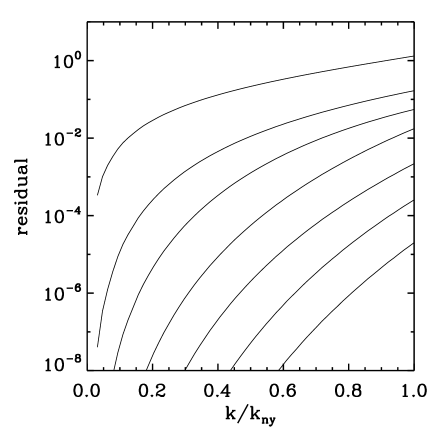
To illustrate quantitatively these results in the $D=3$ case, Figure 2 shows the angular averages of the biases $\Upsilon^{2}(k,0)-1$, $W_{N}(k)-1$ (left panel) and the residual $R_{N}(k)$ as functions of $|k|$ for various values of $N$. More specifically, and this will be used further for 3D measurements, one estimates for each integer wavevector $kN_{\rm g}/(2\pi)$ the following quantity

$${\tilde{k}}(k)=E\left(\left|\frac{kN_{\rm g}}{2\pi}\right|+\frac{1}{2}\right),$$ (36)

where $E(x)$ is the integer part of $x$. Then, the angular average of quantity ${\tilde{A}}({\bar{k}})$ for integer wavenumber modulus ${\bar{k}}$ is given by

$${\tilde{A}}({\bar{k}})\equiv\frac{1}{C({\bar{k}})}\sum_{k|{\tilde{k}}(k)={\bar{k}}}A(k),$$ (37)

where the count $C(k)$ is

$$C({\bar{k}})\equiv\sum_{k|{\tilde{k}}(k)={\bar{k}}}1.$$ (38)

This gives the number of integer wavenumbers verifying ${\tilde{k}}(k)={\bar{k}}$. Note that angular averages make sense only if one assumes statistical isotropy, which then means that the power spectrum depends only on $|k|$. This is theoretically the case of the cosmological random fields considered in this work.

The way the angular average is performed here is very rough, and itself introduces some biases with respect to the estimate of the true angular average of the power spectrum. Implementation of a better angular averaging procedure would be quite straightforward and easy to propagate in the analytic calculations, but would not serve the purpose of this paper, so we leave it for future work.

Figure 2 shows that the residual function $R_{N}(k)$ decreases rapidly with $N$. It is supplemented with Table 2, which provides numerical values for $k=k_{\rm ny}/2$ and $k=k_{\rm ny}$. One can already see the virtue of the Fourier-Taylor method: going to higher order reduces these otherwise uncontrollable effects, which are clearly not negligible at all for the traditional NGP method ($N=0$) where the residual is of order unity at the Nyquist frequency and still about 20 percent at half the Nyquist frequency, whereas the third-order Fourier-Taylor correction reduces it to about 2 percent and $6\times 10^{-5}$, respectively.

Table 2: Numerical estimate in the 3 dimensional case of the residual function $R_{N}(k)$ after angular average as explained in the text. The calculation has been performed with $N_{\rm g}=128$ but the results should not change significantly for other values of $N_{\rm g}$ as long as they are not too small. The first column indicates the order $N$ of the Taylor expansion, while the second and the third one give $R_{N}(k_{\rm ny}/2)$ and $R_{N}(k_{\rm ny})$, respectively.

$N$	$R_{N}(k_{\rm ny}/2)$	$R_{N}(k_{\rm ny})$
0	0.22	1.3
1	0.011	0.17
2	1.3 $10^{-3}$	0.055
3	5.6 $10^{-5}$	0.018
4	2.0 $10^{-6}$	2.2 $10^{-3}$
5	5.2 $10^{-8}$	2.6 $10^{-4}$
6	1.1 $10^{-9}$	2.0 $10^{-5}$

To understand better the scaling of the functions $\Upsilon^{2}_{N}(k,0)-1$ and $W_{N}(k)-1$ with $k$, one can perform the integral of equation (14) in a sphere instead of a cube. For $D=3$, it reads

$$\nu_{N}(k)\simeq\frac{3}{2}\frac{1-(-1)^{N+1}}{(N+1)(N+3)}\left(\frac{3}{4\pi}\right)^{N/3}\left(\frac{\pi|k|}{k_{\rm ny}}\right)^{N}.$$ (39)

This approximation is not accurate enough for practical calculations, but allows one to see that $W_{N}(k)-1$ and $\Upsilon^{2}_{N}(k,0)-1$ scale as $|k|^{N+2}$ for $N$ and $N+1$, $N$ even. For instance, the second and third order scale the same way with $|k|$, as can been seen on top panel of Fig. 2. Note interestingly the bending of the bias for odd $N$ observed when one approaches the Nyquist frequency: this follows from the fact that the sine function cancels at $k=k_{\rm ny}$, unlike the cosine function. Therefore, if one wants to use the brute-force Fourier-Taylor expansion without a bias correction to the power spectrum, it is better to perform it at odd orders.

4 Validation: tests on an $N$-body simulation

In this section, we validate the analytic results derived just above by performing measurements in a CDM $N$-body simulation. The simulation is described in § 4.1, where we also explain how we estimate statistical errors on the measurement of the power spectrum. In § 4.2, biases on the Fourier-Taylor rough estimator are measured and compared to the theoretical predictions in the final stage of the simulation, which should agree well with the assumptions of local Poisson sampling of a stationary random field used in the previous section. In § 4.3, we consider the initial conditions of the simulation, which correspond to a slightly perturbed grid and therefore strongly deviate from local Poisson behavior. Finally, in § 4.4, we propose a nearly unbiased estimator that should work in all the cases, disregarding the aliasing effects on the power spectrum, which are controlled by the order of the Fourier-Taylor expansion as well as the ratio of $k/k_{\rm ny}$ where $k_{\rm ny}$ is the Nyquist frequency of the grid used to perform the calculations.

4.1 The CDM GADGET sample

Figure 3: A thin slice, $L/128$ thick, extracted from the initial conditions and the final stage of our $128^{3}$ CDM GADGET simulation. On the left panel, because of the strong deviations from local Poisson behavior brought by the grid pattern, the validity of our calculations for the power spectrum biases are questionable. On the right panel, the effects of the grid are much less present, although still visible in underdense regions: they should have much less impact on the measurements.

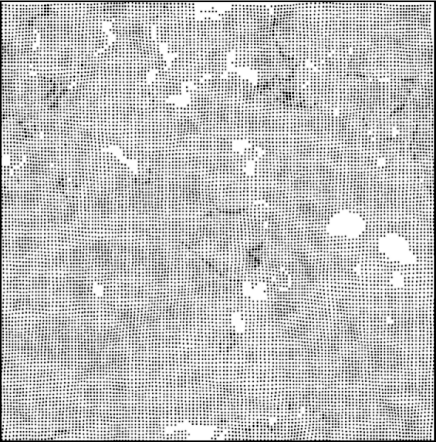
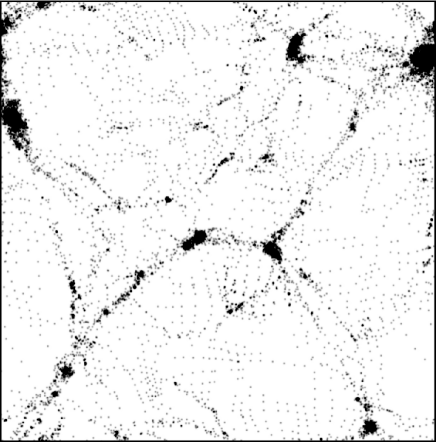
We now validate the above results using a Cold Dark Matter (CDM) $N$-body simulation performed with the publicly available tree code GADGET (Springel, Yoshida & White, 2001), as shown in Fig. 3. The parameters of this simulation are the following. It uses $N_{\rm p}=128^{3}$ particles in a periodic box of size $L=50\ h^{-1}$ Mpc, where $h=H_{0}/(100\mathrm{km}/\mathrm{s}/\mathrm{Mpc})=0.7$. The cosmological parameters are matter density $\Omega_{\rm m}=0.3$ and cosmological constant $\Omega_{\Lambda}=0.7$. The linear variance $\sigma_{8}^{2}$ of the density fluctuations in a sphere of radius $8\ h^{-1}$ Mpc extrapolated to present time was taken to be $\sigma_{8}=0.92$. Finally, the softening length $\varepsilon$ was chosen to be $1/20$th of the mean interparticle distance. The initial conditions were generated using the Graphic package of Berstchinger (2001), with a transfer function given by Bardeen et al. (1986) (no baryons). This package basically allows one to perturb an initially homogeneous particle distribution using the Zel’dovich approximation (Zel’dovich, 1970). For the initial pattern, we chose to put the particles on a regular grid (see left panel of Fig. 3). Our test sample is somewhat small compared to contemporary numerical experiments, but was chosen such that we could perform “exact” calculations of power spectra in a reasonable amount of time. By exact, we mean the 20th order Fourier-Taylor expansion using an $N_{\rm g}=128$ grid. To be able to probe the highly nonlinear regime well and to make sure that the system has properly relaxed to a locally Poissonian and isotropic stage in collapsed objects (see right panel of Fig. 3), we purposely used a small box size.

Figure 4: The power spectrum measured in the initial conditions (lower curves) and the last snapshot, corresponding to the present time (upper curves), of our $128^{3}$ CDM GADGET sample. The symbols correspond to the “exact” measurement with the Fourier-Taylor method of order 20. A shaded region is superposed on them. This represents uncertainties on the measurements as computed from equation (40). The smooth curve gives the non-linear ansatz of Peacock & Dodds (1996). The horizontal dotted line corresponds to the white noise level of the particle distribution. Note that for the measurement at the present time, a correction for white noise was performed, but not for the initial conditions measurement. The bending of the power spectrum at high $k$ in the latter case is due to the Hanning filtering performed in the Graphic package of Berstchinger (2001).

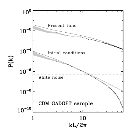
The “exact” power spectrum of the particle distribution in this sample is shown in Fig. 4, both for the initial conditions and the final stage of the simulation. The smooth curves correspond to the nonlinear ansatz of Hamilton et al. (1991) using the formula of Peacock & Dodds (1996), shown here for reference. The error bars represented by the gray shadded areas correspond to the following self-consistent estimate of the statistical error:

$$E^{2}({\bar{k}}) = \left(\frac{\Delta{\tilde{P}}_{\rm rough}({\bar{k}})}{{\tilde{P}}_{\rm rough}({\bar{k}})}\right)^{2}$$ (40)

$$= \frac{1}{C({\bar{k}})[C({\bar{k}})-1]}\times$$

$$\times\left[\sum_{k/{\tilde{k}}(k)={\bar{k}}}(\delta_{k}\delta_{-k})^{2}-C({\bar{k}}){\tilde{P}}^{2}_{\rm rough}({\bar{k}})\right],$$

where

$${\tilde{P}}_{\rm rough}({\bar{k}})=\frac{1}{C({\bar{k}})}\sum_{k/{\tilde{k}}(k)={\bar{k}}}\delta_{k}\delta_{-k}$$ (41)

is the rough power spectrum measured from the distribution of particles. From now on we omit the cumbersome tilde on ${\tilde{P}}$ and bar on ${\bar{k}}$ as we shall only consider angular averages until the end of this section. In the framework of an isotropic, stationary local Poisson process discussed in § 3, recall that after ensemble averaging over many realizations

$$\langle P_{\rm rough}(k)\rangle=P(k)+\frac{1}{N_{\rm p}},$$ (42)

where $P(k)$ is the underlying power spectrum. We noticed that the error given by equation (40) is well-approximated by the well-known result obtained for a random Gaussian field (e.g., Feldman, Kaiser & Peacock, 1994)

$$E^{2}_{\rm G}(k)=\frac{1}{C(k)},$$ (43)

which translates, for the desired shot-noise-corrected power spectrum to

$$\left(\frac{\Delta P}{P}\right)^{2}=\frac{1}{C(k)}\left[1+\frac{2}{N_{\rm p}P(k)}+\frac{1}{N_{\rm p}^{2}P^{2}(k)}\right].$$ (44)

Here, $C(k)$ represents the number of statistically-independent available wavenumbers, hence the missing factor of two compared to the usual case, since symmetries in $k$-space are already taken into account. We are a bit puzzled by the very good agreement between equation (40) and (43), as we would expect non-Gaussian contributions to the error in equation (40) due to nonlinear coupling generated by the dynamics. It seems that these couplings are rather small, as already noticed by Rimes & Hamilton (2006) and Hamilton, Rimes & Scoccimarro (2006). Of course, we know for sure that the error given by equation (40) and (43) underestimate the true value in general, that would be obtained from the dipersion over many realizations of our simulation (Scoccimarro, Zaldarriaga & Hui, 1999). However, the realistic calculation of such an error requires prior knowledge of the bispectrum and the trispectrum. Moreover, eqs. (40) and (43) are sufficient to prove the points discussed in the analyses of this paper and to provide a rough estimate of errors in a simple and self-consistent way, as can be provided by the numerical package we propose.

Due to the very small size of the box, the agreement between the smooth curves and the measurement on Fig. 4 is not very good at large scales (small $k$), where few individual modes are available; this effect is even worse at the final stage of the simulation because of the nonlinear coupling at scales close to the simulation box size. Note importantly that the choice of a regular pattern combined with the Zel’dovich approximation for the initial particle distribution has a non-trivial influence on the evolution of individual modes (Marcos et al., 2006; Joyce & Marcos, 2007a,b; see also Crocce, Pueblas & Scoccimarro, 2006, who discuss transients coming from using the Zel’dovich approximation). Note also that the damping of the power spectrum at large $k$ measured in the initial conditions is not due to any interpolation effect — as we have access here to an “exact” measurement — but to the Hanning filtering performed in Graphic (see Bertschinger, 2001). Finally, while a shot-noise correction was performed on the $P(k)$ obtained in the final stage of the simulation, i.e., a term $1/N_{\rm p}$ was subtracted from the rough measurement, we reiterate that it does not apply to the initial stage. In this case, it is more appropriate to perform no correction as we are in the situation of a perturbed grid pattern (e.g., Joyce & Marcos, 2007a).

4.2 The ideal situation: final, relaxed stage

Figure 5: The measured bias, $b(k)$ (equation 46), on the rough estimator of the power spectrum, $P^{(N)}(k)$, as a function of $k$ for our CDM GADGET sample (symbols). Each panel corresponds to a value of the order $N$, as indicated. The solid and dotted curves represent a theoretical lower and upper bound, respectively, in between which the symbols should lie [equation 46 with $P_{\rm max}=P(k_{\rm ny})$], in the framework of § 3 — local Poisson sampling of an isotropic stationary random field. The shaded region represents the statistical error computed from equation (40).

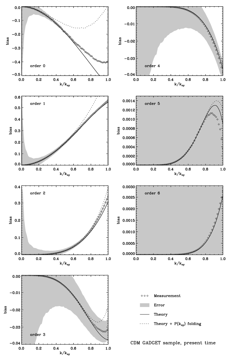
Figure 5 shows the measured bias on the shot-noise-corrected measured Fourier-Taylor power spectrum of order $N$, for various values of $N$:

$$b(k)=\frac{P^{(N)}(k)-W_{N}(k)/N_{\rm p}-P(k)}{P(k)}.$$ (45)

If the analytic calculations of § 3.2 apply, we should have

$$\gamma_{N}^{2}(k,0)\mathrel{\mathchoice{\vbox{\offinterlineskip\halign{\hfil$\displaystyle#$\hfil\cr<\cr\sim\cr}}}{\vbox{\offinterlineskip\halign{\hfil$\textstyle#$\hfil\cr<\cr\sim\cr}}}{\vbox{\offinterlineskip\halign{\hfil$\scriptstyle#$\hfil\cr<\cr\sim\cr}}}{\vbox{\offinterlineskip\halign{\hfil$\scriptscriptstyle#$\hfil\cr<\cr\sim\cr}}}}b(k)\mathrel{\mathchoice{\vbox{\offinterlineskip\halign{\hfil$\displaystyle#$\hfil\cr<\cr\sim\cr}}}{\vbox{\offinterlineskip\halign{\hfil$\textstyle#$\hfil\cr<\cr\sim\cr}}}{\vbox{\offinterlineskip\halign{\hfil$\scriptstyle#$\hfil\cr<\cr\sim\cr}}}{\vbox{\offinterlineskip\halign{\hfil$\scriptscriptstyle#$\hfil\cr<\cr\sim\cr}}}}\gamma_{N}^{2}(k,0)+\frac{P_{\rm max}}{P(k)}[W_{N}(k)-\Upsilon_{N}^{2}(k,0)].$$ (46)

The lower and upper bound are represented by the continuous and the dotted line respectively. We assume $P_{\rm max}=P(k_{\rm ny})$. As expected, within the statistical errors defined by equation (40), the measurements represented by the symbols indeed lie in between these two curves. Since the true power spectrum is a strongly decreasing function of $k$ in the CDM cosmology, the effects of aliasing of the power spectrum are overestimated by the dotted curve, so the symbols are much closer to the solid curve than to the dotted one. In fact, they overlay quite well on the solid curve when $k$ is small enough compared to $k_{\rm ny}$, as expected. Note that the nearest grid point interpolation (upper left panel) is still very significantly contaminated by aliasing, while this effect decreases rapidly with the order $N$ as shown in previous section. The bias also becomes smaller and smaller with $N$, but it is really worth correcting for, since the theoretical predictions match rather well the measurements. Note that at high order, $N\geq 4$, the symbols no longer lie between the dotted and solid curve, but this is nonetheless well within the statistical errors represented as the shaded region. Moreover, the system still deviates locally from a pure random stationary pattern (right panel of Fig. 3) so one cannot expect the theoretical bound given by equation (46) to remain valid at such a level of accuracy.

4.3 A poor situation: a perturbed grid as in the initial stage

Figure 6: Same as Fig. 5, but the function displayed is now $g(k)$ (equation 47) as measured in the initial conditions of our GADGET sample, which correspond to a perturbed grid. The solid lines on each panel still show function $\gamma^{2}_{N}(k,0)$, while the dotted line gives $\gamma^{2}_{N}(k,0)+(P_{\rm rough}(k)N_{\rm p})^{-1}[W_{N}(k)-\Upsilon_{N}^{2}(k,0)]$ as discussed in the text.

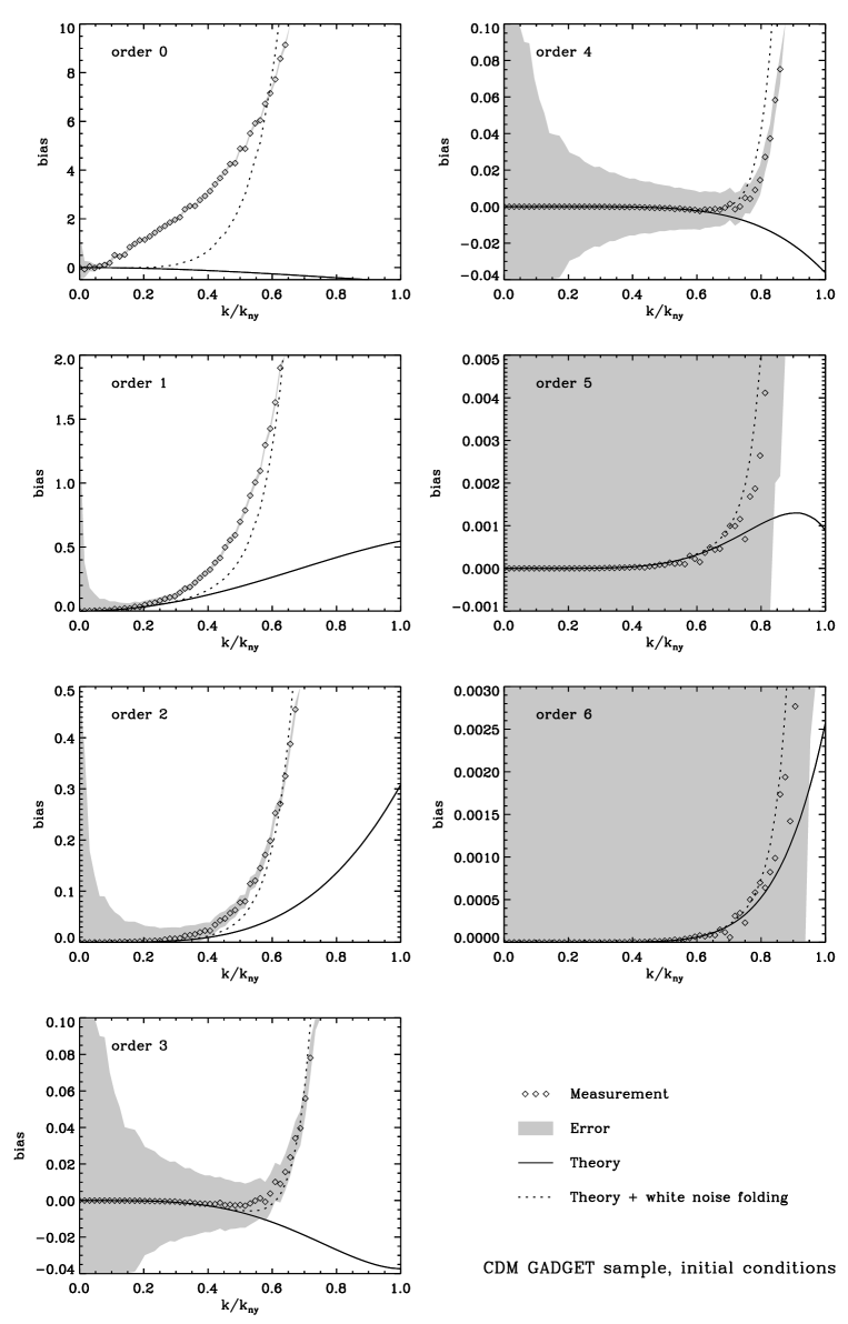
While the final stage of our GADGET sample is well within the framework of the assumptions of local Poisson sampling of a stationary random process, this is not the case for the initial conditions, which correspond to a slightly perturbed grid pattern, as shown on left panel of Fig. 3. Fig. 6 is the same as Fig. 5, but now the function measured is

$$g(k)=\frac{P^{(N)}(k)-P_{\rm rough}(k)}{P_{\rm rough}(k)}.$$ (47)

In other words, no correction for the shot-noise of the particles is performed since it does not make sense in that case.

Before pushing this analysis further, we have to understand what is the particle sample at hand. The Graphic package perturbs an initial grid pattern with a Gaussian random displacement field, ${\cal P}(q)$, supposed to be stationary, isotropic and curl-free. We assume, to simplify the discussion which follows, that the grid of particles is the same as the grid used to perform fast Fourier transforms, $N_{\rm p}=N_{\rm g}^{3}$. This is the case for Fig. 6. Remember finally that lengths are expressed in units of the size of the a cell of the grid.

The perturbed position of the particle is given by

$$x=s+q+{\cal P}(q),$$ (48)

where $q$ is an integer vector for which each coordinate is in the range $[0,N_{\rm g}-1]$, and $s$ is a small constant offset, for which each coordinate is in $[0,1[$. Usually, $s=0$ or $s=(0.5,0.5,0.5)$. The Fourier mode of the perturbed grid pattern is given by

$$\delta_{k}=\frac{1}{N_{\rm p}}\sum_{q}\exp\{Ik\cdot[s+q+{\cal P}(q)]\}.$$ (49)

While it is possible to compute the exact power spectrum of such a perturbed grid (Gabrielli, 2004, see Appendix C and equation 50 below), the general calculation for the Fourier-Taylor expansion is very cumbersome. However, three interesting regimes can at least partly be discussed qualitatively:

1. Very small displacement, $\sigma^{2}\equiv\langle{\cal P}^{2}\rangle\ll 1$: in that case, the value of $s$ controls the amplitude of the displacement $\Delta(i)$ in equation (5) and therefore the accuracy of the Fourier-Taylor expansion. The smaller $s$, the better. The worst situation is when $s$ approaches diagonal values, e.g., $s=(0.5,0.5,0.5)$. Therefore, to best exploit the Fourier-Taylor method on a very slightly perturbed grid, it is wise to chose $s$ (and more generally the size of the grid $N_{\rm g}$) carefully, to minimize as much as possible the amplitude of the displacements $\Delta(i)$. In the conventions used here, the wisest choice is thus $s=0$.

2. Significant displacement, $\sigma^{2}\simeq 1$: this is the situation of Fig. 6, where $\sigma\simeq 0.88$. In that case, there will be always a large fraction of particles with large magnitude of the displacement $\Delta(i)$, independently of the choice of the offset $s$.

3. Large displacement, $\sigma^{2}\gg 1$: it is difficult in this case to make any quantitative statements because the conclusions depend on the coherence of the displacement field (see equation 50 below). However, one can postulate in general that the information due to the grid pattern has become subdominant: the particle distribution should behave again like the local Poisson realization of an isotropic stationary random process and the calculations of § 3 should in practice become valid again.

From this simple discussion, which could be easily extended to the more general case $N_{\rm p}\neq N_{\rm g}^{3}$, one sees that the measurement of the power spectrum on a perturbed grid has to be performed carefully in order to reduce as much as possible the systematic errors on the Fourier-Taylor spectrum. However, one expects these errors to become significant only when approaching the Nyquist frequency.

This is well illustrated by Fig. 6, for which we have $s=(0,0,0)$ and a mean square displacement of order unity [point (ii) above]: the magnitude of function $g(k)$ increases quite rapidly when $k/k_{\rm ny}$ approaches unity. The solid line on each panel still represents the function $\gamma_{N}^{2}(k,0)$. The dotted line corresponds to the right member of equation (46), but with $P_{\rm max}=1/N_{\rm p}$. This gives a good idea of the overall behavior of $g(k)$, and this is not very surprising. Indeed the calculations of Appendix C (see also, e.g., Gabrielli, 2004) give

$\langle\delta_{k}\delta_{-k}\rangle=\delta_{\rm D}(0)\ +$

$$\hbox{}\quad\quad+\frac{1}{N_{\rm p}}\sum_{q}\exp(Ik\cdot q)\exp\left\{-\frac{k^{2}\sigma^{2}}{3}\left[1-\rho(q)\right]\right\},$$ (50)

where $-1\leq\rho(q)\leq 1$ is the correlation coefficient of the displacement field. From this equation, one sees that for a moderately perturbed grid ($\sigma^{2}\mathrel{\mathchoice{\vbox{\offinterlineskip\halign{\hfil$\displaystyle#$\hfil\cr<\cr\sim\cr}}}{\vbox{\offinterlineskip\halign{\hfil$\textstyle#$\hfil\cr<\cr\sim\cr}}}{\vbox{\offinterlineskip\halign{\hfil$\scriptstyle#$\hfil\cr<\cr\sim\cr}}}{\vbox{\offinterlineskip\halign{\hfil$\scriptscriptstyle#$\hfil\cr<\cr\sim\cr}}}}1$), the power spectrum presents a peak at twice the Nyquist frequency of the grid. The amplitude of this peak is controlled by the amplitude of the displacements, i.e., the value of $\sigma$. However, when $k^{2}\gg 1/\sigma^{2}$, the sum in equation (50) is dominated by the $q=0$ term, hence

$$\langle\delta_{k}\delta_{-k}\rangle\simeq\frac{1}{N_{\rm p}},\quad k^{2}\gg 1/\sigma^{2}.$$ (51)

This means that at wavenumbers large enough, the rough power spectrum of the perturbed grid is dominated by the shot noise of the particles. Since $\sigma\sim 1$ in our experiment, this should happen for $k^{2}$ approaching a few units (except for the peak just mentioned above at twice the Nyquist frequency of the grid). As a result, the effects of the aliasing of the power spectrum should be roughly of the order of the shot noise, which is indeed the case on Fig. 6: the symbols follow roughly the dotted curve, except perhaps for the nearest grid point case (upper left panel).

Despite the much stronger effects of aliasing on the Fourier-Taylor spectrum for the perturbed grid than for the locally Poissonian case, the systematic errors on $P^{(N)}(k)$ still decrease rapidly with the order, $N$. They remain quite moderate when $k/k_{\rm ny}$ is kept small enough, for instance $k/k_{\rm ny}\mathrel{\mathchoice{\vbox{\offinterlineskip\halign{\hfil$\displaystyle#$\hfil\cr<\cr\sim\cr}}}{\vbox{\offinterlineskip\halign{\hfil$\textstyle#$\hfil\cr<\cr\sim\cr}}}{\vbox{\offinterlineskip\halign{\hfil$\scriptstyle#$\hfil\cr<\cr\sim\cr}}}{\vbox{\offinterlineskip\halign{\hfil$\scriptscriptstyle#$\hfil\cr<\cr\sim\cr}}}}1/2$ for third order, $N=3$, and increase rapidly if $k$ approaches the Nyquist frequency.

4.4 Unbiased estimator: a zoom in the range $[0,k_{\rm ny}/2]$

From equation (31) we can write an angle-averaged estimator of the true power spectrum:

$$P_{\rm est}^{(N)}(k)=\left\langle\frac{P^{(N)}(k)}{\gamma^{2}_{N}(k,0)}-\frac{R_{N}(k)+1}{N_{\rm p}}\right\rangle_{\rm angles}.$$ (52)

Recall that the second term of the right side of this equation has to be ignored if we consider a perturbed regular pattern such as initial conditions of a $N$-body simulation. We explicitly write the angular average in this expression, to show how it should be performed to get the best estimate of $P(k)$. Equation (52) gives the estimator we propose in that paper.

Figure 7: A zoom in the region $[0,k_{\rm ny}/2]$ of the relative residual, $\delta P(k)/P(k)=[P_{\rm est}^{(N)}-P(k)]/P(k)$, on the unbiased third-order power spectrum, as measured in our CDM GADGET sample. The upper panel corresponds to present time, where shot-noise correction was performed, while the lower one corresponds to initial conditions, with no shot noise correction.

In the next section, we shall present a procedure to extend the dynamic range of available values of $k$, which has been restricted up to now the the Nyquist range of the (arbitrary) sampling grid used to perform the Fourier-Taylor transform. This method will allow us to control the accuracy of the measurements at all wavenumbers, except of course those corresponding to modes close to the box size. The previous analyses suggest keeping $k$ far away enough from $k_{\rm ny}$. The choice proposed in this paper is $k\leq k_{\rm ny}/2$. Figure 7 shows the relative residual on the third-order unbiased estimator in the region $k\in[0,k_{\rm ny}/2]$. Such a residual is well below the statistical errors, of the order of $1.5\times 10^{-4}$ and $4\times 10^{-3}$ at most in the final and the initial stage of the simulation respectively. This error, already small, can be reduced further by increasing the order $N$. However, it does not make sense to do so as long as the statistical errors are dominant: to reduce the statistical errors one has to sample more modes, i.e., to increase the size of the grid used to perform the Fourier-Taylor transform. This is discussed in next section.

5 Arbitrary wavenumbers with controlled error

In this section, we show how the dynamical range of available values of $k$ can be increased arbitrarily while keeping the statistical errors and the aliasing effects on the measurements bounded (Jenkins et al., 1998).

As shown above, the error on the Fourier-Taylor expansion is basically controlled by the magnitude of $k$: this latter has to remain a small enough fraction of the Nyquist frequency to avoid uncontrollable effects of aliasing and hence to be able to maintain sufficiently low order $N$. Assuming that $\delta_{k}$ was computed in a given range of values of (each coordinate of) $k$, $[-\alpha k_{\rm ny},\alpha k_{\rm ny}]$, $\alpha\leq 1$, one can now consider an arbitrary shift, $k_{s}$, such that $k+k_{s}$ is outside the available range, e.g., $k_{s}=2\alpha k_{\rm ny}$ to have access to the range $[\alpha k_{\rm ny},3\alpha k_{\rm ny}]$ in 1D. Equation (2) is rewritten

$$\delta_{k+k_{s}} = \frac{1}{N_{\rm p}}\sum_{i}M_{i}\exp(Ik\cdot x_{i})\exp(Ik_{s}\cdot x_{i}),$$ (53)

$$= \frac{1}{N_{\rm p}}\sum_{i}M^{\prime}_{i}\exp(Ik\cdot x_{i}),$$ (54)

with

$$M^{\prime}_{i}=M_{i}\exp(Ik_{s}\cdot x_{i}).$$ (55)

One thus obtains, by simple multiplication of the weights by $\exp(Ik_{s}.x_{i})$, a modification of the Fourier-Taylor algorithm that gives access to arbitrary values of $k$ while maintaining the errors bounded. Of course, a new set of $N_{\rm FFT}$ transforms has to be performed for each value of $k_{s}$.

While this method allows us to investigate arbitrary values of $k$, there is still the limitation imposed by the available computer resources. For instance increasing the computing volume from a cube of sides $[-k_{\rm ny},k_{\rm ny}]$ to a cube of sides $[-M\ k_{\rm ny},M\ k_{\rm ny}]$ amounts to a calculation $M^{D}$ times more expensive than for the original data cube. Instead, one can notice the following property of Fourier transform in one dimension. Writing

$$\delta_{2k} = \frac{1}{N_{\rm p}}\sum_{i}\exp(2Ikx_{i})$$ (57)

$$= \frac{1}{N_{\rm p}}\sum_{i,x_{i}\in[0,L/2[}\exp(2Ikx_{i})+$$

$$+\frac{1}{N_{\rm p}}\sum_{i,x_{i}\in[L/2,L[}\exp[2Ik(x_{i}-L/2)+IkL],$$

we can set

$$r_{i} = 2x_{i}\ {\rm for}\ x_{i}\in[0,L/2[,$$

$$r_{i} = 2x_{i}-L\ {\rm for}\ x_{i}\in[L/2,L[.$$ (58)

We then have

$$\delta_{2k}=\frac{1}{N_{\rm p}}\sum_{i}\exp(Ikr_{i}),$$ (59)

if we assume that $kL/(2\pi)$ is an integer; in that case $\exp(IkL)=1$. Similarly one can write

$$\delta_{2k+1}=\frac{1}{N_{\rm p}}\sum_{i}S(i)\exp(Ikr_{i}),$$ (60)

where the sign function $S(i)$ satisfies

$$S(i) = \,\,\,\,\,1,\,\,{\rm if}\,\,x_{i}\in[0,L/2[,$$ (61)

$$S(i) = -1,\,\,{\rm if}\,\,x_{i}\in[L/2,L[.$$ (62)

This means that we now have access to a doubly-large range of integer values of $kL/(2\pi)$ by applying Fourier-Taylor method on simple foldings of the particle distribution. Note that periodicity is not assumed here, except that only the integer values of $kL/(2\pi)$ are available. Such a set is complete in the periodic case.

Table 3: The sampled values of $kL/(2\pi)$ when using the folding procedure explained in the main text on a grid with $N_{\rm g}=16$. The trivial fundamental case, $k=0$, is not shown here. From the left column to the right one, one considers $M=0$ folding to $M=4$ foldings. Each column defines a range of available values of $k$. As discussed in the text, there can be several estimates of $P(k)$ for a given value of $k$. For instance we have 3 estimates of $P(4)$. To make unknown aliasing effects always negligible in practice compared to statistical errors, we impose $k\leq k_{\rm ny}^{(M)}/2$, where $k_{\rm ny}^{(M)}$ is the effective wavenumber probed by the Nyquist frequency of the grid after $M$ foldings (this is indicated by the mid-horizontal line on the table). To minimize the statistical errors, $M$ should then be as small as possible, since this parameter controls the sparseness of sampling in Fourier space. To measure $P(4)$ for instance, one takes $M=0$. In detail, the sampled values of $k$ are highlighted in bold on the table, $k=1,2,4,6,8,12,16,24,32,48,64$; Fourier space is increasingly sparse sampled with $k$. This sparse sampling roughly increases linearly in logarithmic scale, but the width of the bin used to measure $P(k)$ increases likewise, keeping the number of sampled independent modes $C(k)$ bounded between two values $C_{1}$ and $C_{2}$ independent of the number of foldings $M$, except for $M=0$ [here $C_{1}=98$ and $C_{2}=210$ for $D=3$]. As a result, the statistical errors on the power spectrum measurement remain bounded as well, as illustrated by Fig. 9.

$M=0$	$M=1$	$M=2$	$M=3$	$M=4$	$C(k)\ (D=3)$
1	2	4	8	16	18
2	4	8	16	32	62
3	6	12	24	48	98
4	8	16	32	64	210
5	10	20	40	80	350
6	12	24	48	96	450
7	14	28	56	112	602
8	16	32	64	128	762

Obviously this folding trick can be generalized to higher number of dimensions. In that case, the number of Fourier transforms needed to perform the calculations increases by a factor $2^{D}$ each time a factor 2 is gained in the dynamic range of available values of $k$, exactly as in equations (54) and (55), as expected. However, we can restrict here to the simplest folding given by equation (59) and ignore foldings involving equation (60). This means that we are sparse-sampling Fourier space, increasing the dynamic range by a factor two each time, maintaining the computational time of the same order at each step of the procedure. Table 3 shows the list of values of $k$ sampled in one dimension in a simple case, where $N_{\rm g}=16$. Note that the number of available modes per sampled value of $k$ remains the same as for the original sampling: the error on the rough power spectrum shall remain bounded as we discuss later below.

In practice the folding algorithm works as follows:

1. First apply the Fourier-Taylor estimator on the original particle distribution sampled on the periodic grid of size $N_{\rm g}$, and measure $P_{\rm est}^{(N)}(k)$ up to some fraction of the Nyquist frequency, $\alpha k_{\rm ny}$, with e.g., $\alpha=1/2$ as advocated in the previous section. That corresponds to the first step of the algorithm, with zero folding, $M=0$.

2. (Assuming we are at step $M$ of the process.) Fold the particles in each dimension according to equation (58), resample them again on a periodic grid of size $N_{\rm g}$, but which probes a physical size twice smaller than in the previous step, $L_{M+1}=L_{M}/2=L_{0}/2^{M+1}$ ($L_{0}=L$). Measure $P_{\rm est}^{(N)}(k)$ up to $\alpha$ times the Nyquist frequency of that grid, which in practice corresponds to twice the Nyquist frequency of the grid of the previous step, $k_{\rm ny}^{(M+1)}=2k_{\rm ny}^{(M)}=2^{M+1}k_{\rm ny}$.

3. Repeat step (ii), until the value $\alpha k_{\rm ny}^{(M+1)}$ is as large as required, for instance until the softening scale of the simulation has been reached.

We now have a set of values of measurements of the power spectrum for a number of ranges of values of $k$ as for instance illustrated by Table 3. These ranges overlap from one folding to another: this can be used to check for systematic errors on the measurements. Indeed, for one value of $k$, there can be several measurements of $P(k)$. One has, for each folding, to choose the range of values of $k$ that contribute to the final measurement. To do that, one could think of compromising between the statistical errors, which are larger when $k$ is small, and the unknown systematics brought by aliasing, which can become significant when $k$ approaches the Nyquist frequency of the grid. The choice of compromise depends on the order $N$ of the Fourier-Taylor transform considered. It is theoretically possible to find an “optimal” compromise between the parameter $\alpha$, the order $N$ and the resolution of the grid, $N_{\rm g}$, to maintain the errors on the measurement of $P(k)$ below a given limit at a minimum computational cost. However, such a project would go beyond the scope of this paper. Our strategy here is rather to make sure that the unknown systematics due to aliasing are negligible compared to the statistical error given by e.g., equation (43). We therefore advocate $\alpha=1/2$ and sufficiently high order Fourier-Taylor approximation. For instance, the third-order transform should in practice do well enough for $N_{\rm g}$ of the order or smaller than a thousand.

Figure 8: The power spectrum measured at present time in our CDM GADGET sample, with the estimator $P^{(3)}_{\rm est}(k)$ (equation 52), using the folding algorithm explained in the main text to (sparsely) probe the full dynamic range $k=[1,8192]$. To see the details better, the measurements have been divided by the analytical proxy $P_{\rm PD}(k)$ of Peacock & Dodds (1996). Each panel corresponds to a choice of the grid resolution, $N_{\rm g}$, used to perform the Fourier-Taylor algorithm in combination with the folding of the particle distribution. The measurements are represented by the thin curve, while the shaded region gives the statistical error estimated with equation (40). The dashed curve corresponds to the shot noise of the particles. The dotted vertical line indicates the softening length $\varepsilon$: above that scale, $P(k)$ should present a cut-off, which is clearly visible when the signal-to-noise ratio is large enough, see e.g., the lower-right panel.

Figure 9: The statistical error on the measurement of $P(k)$ when using the folding procedure explained in the main text. The upper curves correspond to the estimated statistical relative error on $P^{(3)}_{\rm est}(k)$ (but these curves would not change significantly for other values of the order $N$ of the Fourier-Taylor expansion): for various values of $N_{\rm g}$ as indicated on the plot, the thin (alternatively dotted and solid) and the thick grey curves correspond respectively to eqs. (40) and (43) for estimating the errors on the measurement of $P(k)+1/N_{\rm p}$. The function represented here is given in fact by equation (63) as discussed in detail in the main text. For comparison, the lower curves give an estimate of the expected residual due to aliasing effects on the power spectrum, while the symbol show the measurement of these residuals for $N_{\rm g}=128$.

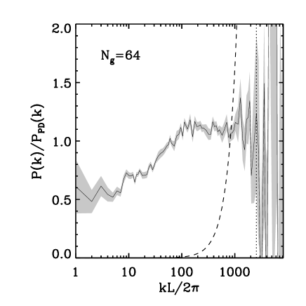
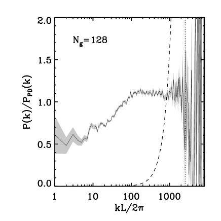
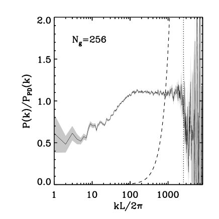
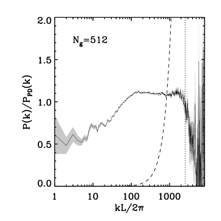
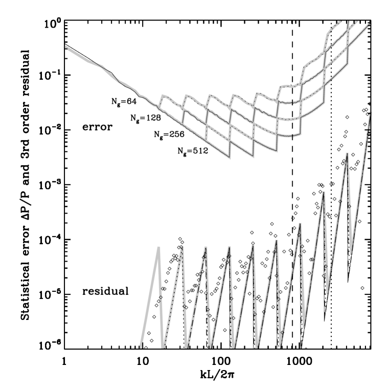
Figure 8 illustrates how the measurements behave over the range $kL/(2\pi)\in[1,8192]$ when one changes the grid resolution from $N_{\rm g}=64$ to $N_{\rm g}=512$ in the folding algorithm. In order to see the details better, the function represented on each panel is $P^{(3)}_{\rm est}(k)/P_{\rm PD}(k)$, where $P_{\rm PD}(k)$ is the function given by the nonlinear ansatz of Peacock & Dodds (1996). This figure is supplemented with Fig. 9, which gives for each case considered in Fig. 8 the errors on $P^{(3)}_{\rm est}(k)$, in the following way to make the plot readable: the thin curve (alternatively dotted and continuous) and the thick grey curves on the upper part of Fig. 9 correspond to equations (40) and (43) respectively. However these equations give the error on the estimate of the power spectrum plus the shot noise contribution of the particles. In order to get an estimate of the statistical error on $P(k)$, we compute an expression similar to equation (44), but as follows:

$$\frac{\Delta P}{P}=\left\{E(k)\ {\rm or}\ E_{\rm G}(k)\right\}\times\frac{P_{\rm PD}(k)+1/N_{\rm p}}{P_{\rm PD}(k)}.$$ (63)

That way, the plot is readable because we replace a noisy function with its smooth guess $P_{\rm PD}(k)$. The lower part of the same figure shows the residual function due to aliasing, $R_{3}(k)\{1+1/[P_{\rm PD}(k)N_{\rm p}]\}$ (thick grey, dotted, dashed and solid lines, which correspond to $N_{\rm g}=64$, 128, 256 and 512, respectively), as well as its measurement for $N_{\rm g}=128$ (symbols). In the last case, the function displayed on Fig. 9 is $[P^{(3)}_{\rm est}(k)-P(k)]/P_{\rm PD}(k)$. It should roughly follow the dotted line, which is indeed the case. Note that a residual $f(k)=R_{3}(k)\{1+1/[P_{\rm PD}(k)N_{\rm p}]\}$ assumes $P_{\rm max}=P_{\rm PD}(k)$. Since $P_{\rm PD}(k)$ is a decreasing function of $k$, the function $f(k)$ is expected to overestimate the true residual. On the contrary, the symbols tend to lie above the “theory”, but this disagreement is clearly within statistical errors, which is what really matters for the point made here.

The mid-range values of $k$ in Fig. 9 show that increasing the resolution $N_{\rm g}$ of the grid by a factor of two improves the overall signal-to-noise ratio by a factor $2^{(D-1)/2}$, because $C(k)$ scales roughly like $k^{D-1}$. This is illustrated as well by Fig. 8, where the small fluctuations of the measured spectrum at intermediate values of $k$ decrease when $N_{\rm g}$ increases. At small $k$, however, the errors are independent of $N_{\rm g}$ as there are fewer and fewer statistically independent modes when one approaches the size of the box, whatever the resolution of the grid used to perform the measurements. At large $k$, one is dominated by the shot noise of the particles: when $P(k)\mathrel{\mathchoice{\vbox{\offinterlineskip\halign{\hfil$\displaystyle#$\hfil\cr<\cr\sim\cr}}}{\vbox{\offinterlineskip\halign{\hfil$\textstyle#$\hfil\cr<\cr\sim\cr}}}{\vbox{\offinterlineskip\halign{\hfil$\scriptstyle#$\hfil\cr<\cr\sim\cr}}}{\vbox{\offinterlineskip\halign{\hfil$\scriptscriptstyle#$\hfil\cr<\cr\sim\cr}}}}1/N_{\rm p}$, as indicated by the dashed line on Figs. 8 and 9, the error on $P(k)$ increases dramatically, to become arbitrarily large when $P(k)$ is subject to the hard cut-off due to the softening of the forces at scales smaller than $\varepsilon$, as indicated by the dotted line on the figures. Indeed, in the folding method proposed here, one is actually able to control the error on the measurement of the quantity $P(k)+1/N_{\rm p}$, and not on the measurement of $P(k)$.

6 Summary

In this paper we presented a method to estimate Fourier modes of a particle distribution, based on a Taylor expansion of the trigonometric functions. This idea is inspired from the work of Anderson & Dahleh (1996). We paid particular attention to the measurement of the power spectrum $P(k)$ when the point distribution is the local Poisson realization of a stationary random field, where explicit expressions for the ensemble average of a naive rough estimator of $P(k)$ were derived. This allowed us to accurately determine the biases induced by discreteness and by the Taylor expansion, which can be easily corrected for, and to quantify the effects of aliasing, which are controlled by the order, $N$, of the expansion. Our calculations show that effects of aliasing decrease quickly with $N$, as illustrated by Table 2. The analytic calculations were confronted successfully with a cosmological $N$-body simulation. We also studied how the deviations from local Poisson behavior influence the measurements, such as in initial conditions of the simulation, which correspond to a perturbed grid pattern. We proposed an unbiased estimator which is nearly free of aliasing, and which still performs well for the perturbed grid. The accuracy of this estimator is thus entirely controlled by the statistical errors, which arise from the finite number of sampled modes. We also showed how the dynamical range in Fourier space could be arbitrarily increased while keeping the statistical error bounded, by appropriate foldings of the particle distribution, as suggested by Jenkins et al. (1998). Note that, while the Fourier-Taylor method was applied here to the power spectrum, it can be easily generalized to higher order estimators, for instance to measure the bispectrum or the trispectrum of the distribution.

The Fourier-Taylor module as well as the associated power spectrum estimator tool we propose is available as an F90 package, powmes, at www.projet-horizon.fr or on request from the authors. It works with the GADGET file format.

Appendix A Ensemble averages with various assumptions

There are subtleties that arise when it comes to performing ensemble averages. While this has been widely discussed in the literature (see, e.g., Peebles 1980), we address the issue briefly again here. Given a distribution of $N_{\rm p}$ particles in a (hyper)cubical volume $V$, which is a discrete realization of an underlying random continuous field, $\rho(x)$ (of average unity), one measures the two quantities

$$F=\sum_{i=1}^{N_{\rm p}}f(x_{i}),\quad G=\sum_{i=1}^{N_{\rm p}}g(x_{i}),$$ (65)

where $f$ and $g$ are some functions. The question we want to address here is how to compute the ensemble average of $FG$ over many realizations of the underlying distribution, given some constraints. There are two relevant cases to consider:

1. The “realistic” case: $V$ is a subvolume of a realization of much larger volume. In that case ensemble average allows the number of particles $N_{\rm p}$ to vary, as well as the average density over the volume: the quantity

   $$\rho(V)=\frac{1}{V}\int_{V}\rho(x)d^{D}x,$$ (66)

   is allowed to fluctuate around the mean.

2. The $N$-body simulation standard case: in that case, $N_{\rm p}$ is fixed, as well as $\rho(V)\equiv 1$.

A.1 The “realistic” case: unconstrained ensemble average

Following Peebles (1980), we divide $V$ into infinitesimal cells of volume $\delta V$, such that they contain zero or one particle. Let $n$ be the number of particles they contain, and ${\bar{n}}=\langle n\rangle$ its ensemble average. Let $p(n,x)$ be the probability of having $n$ particles in an infinitesimal cell at position $x$. Then, the local random process characterizing the realization of the smooth field in a distribution of particles gives, assuming that $\langle\rho\rangle=1$,

$$p(1,x) = {\bar{n}}\delta V\rho(x),$$ (67)

$$p(0,x) = 1-{\bar{n}}\delta V\rho(x).$$ (68)

The sum (65) can be rewritten over the infinitesimal cells, labelled as $j$ and at positions $c_{j}$,

$$F=\sum_{j}n_{j}f(c_{j}),\quad G=\sum_{j}n_{j}g(c_{j}).$$ (69)

So

$$\langle F\rangle=\sum_{j}\langle n_{j}f(c_{j})\rangle=\sum_{j}{\bar{n}}\delta V\langle\rho\rangle f(c_{j}),$$ (70)

which gives in integral notation

$$\langle F\rangle={\bar{n}}\int_{V}d^{D}xf(x),$$ (71)

and likewise for $G$. The product, $FG$, is then

$$FG=\sum_{j}n_{j}^{2}f(c_{j})g(c_{j})+\sum_{j\neq j^{\prime}}n_{j}n_{j^{\prime}}f(c_{j})g(c_{j}^{\prime}).$$ (72)

$$\langle FG\rangle = {\bar{n}}\int_{V}f(x)g(x)d^{D}x+$$ (73)

$$+\ {\bar{n}}^{2}\int_{V}[1+\xi(x,y)]f(x)g(y)d^{D}xd^{D}y.$$

In this equation, we have defined the two-point correlation function

$$\langle\rho(x)\rho(y)\rangle\equiv 1+\xi(x,y).$$ (74)

In this paper, we assume stationarity: $\xi(x,y)=\xi(x-y)$. Equation (73) is the basis that we used for the calculation of the ensemble average of $P^{(N)}(k)$ in § 3.1, and from which we derive equation (24).

A.2 The $N$-body simulation case: constrained ensemble average

Since $N_{\rm p}$ is now fixed, the method of infinitesimal cells does not work anymore, at least not straightforwardly. However, what still remains valid is that the probability of having a particle at position $x$ is proportional to $\rho(x)$. More generally, the probability density of having a set of particles at positions $(x_{1},\cdots,x_{N_{\rm p}})$, given the realization $\rho(x)$, is given by

$$p(x_{1},\cdots,x_{N_{\rm p}})=\frac{1}{V^{n}}\rho(x_{1})\cdots\rho(x_{N_{\rm p}}),$$ (75)

remembering that $\rho(V)$ (equation 66) is now constrained to be unity for each realization of the ensemble average. Then

$$\langle F\rangle = \sum_{i=1}^{N_{\rm p}}\left\langle\int f(x_{i})p(x_{1},\cdots,x_{N_{\rm p}})d^{D}x_{1}\cdots d^{D}x_{N_{\rm p}}\right\rangle$$ (76)

$$= \frac{N_{\rm p}}{V}\int_{V}f(x)d^{D}x,$$

after performing the integrals and then ensemble averaging, using $\langle\rho\rangle=1$. As a result we converge again to equation (71), since ${\bar{n}}=N_{\rm p}/V$. However, the calculation of $\langle FG\rangle$ gives,

$$\langle FG\rangle=\frac{N_{\rm p}}{V}\int_{V}f(x)g(x)d^{D}x+\frac{N_{\rm p}(N_{\rm p}-1)}{V^{2}}\times$$

$$\times\int_{V}[1+\xi(x,y)]f(x)g(y)d^{D}xd^{D}y,$$ (77)

using the definition (74). The second term of this expression differs from second term of equation (73), by a factor $(N_{\rm p}-1)/N_{\rm p}$. In addition, the constraint $\rho(V)=1$ for each realization reads, after ensemble averaging,

$$\int_{V}\xi(x,y)d^{D}xd^{D}y=0.$$ (78)

These differences impose, in particular, that the fundamental mode, $P^{(N)}(0)$ is always exactly unity for an $N$-body simulation in our choices of units, unlike equation (24), which was computed using the method explained in Appendix A1.

Appendix B Some useful analytic expressions

The calculation of the number $\kappa_{n}(k,M)$ (equation 23) can be performed easily by using the multinomial theorem:

$$\kappa_{n}(k,M)=\sum_{q_{1}+\cdots+q_{D}=n}\frac{n!}{q_{1}!\times\cdots\times q_{D}!}\times$$

$$\times\eta_{q_{1}}(k_{1},M_{1})\times\cdots\times\eta_{q_{D}}(k_{D},M_{D}),$$ (79)

where

$$\eta_{n}(k,M)=\int_{-1/2}^{1/2}\exp[-I\ (k+2\pi M)\Delta]\ (I\ k\Delta)^{n}d\Delta$$ (80)

is similar to $\kappa_{n}(k,M)$ but is computed on a scalar instead of a vector: for $D=1$, $\eta_{n}(k,M)=\kappa_{n}(k,M)$. Note that $\eta_{n}(k,M)$ can be computed using the following recursion:

$$\eta_{0}(k,M)=(-1)^{M}\sin(k/2)/[(k+2\pi M)/2],$$ (81)

$$\eta_{n}(k,M)=\frac{(-1)^{M}}{k+2\pi M}({k}/{2})^{n}I\{I^{n}\exp(-I\ k/2)-$$

$$-\ I^{-n}\exp(I\ k/2)\}+\frac{n\ k}{k+2\pi M}\eta_{n-1}(k,M).$$ (82)

The final result can be expressed as

$$\eta_{n}(k,M)=\frac{2(-1)^{M}k^{n}n!}{(k+2\pi M)^{n+1}}\times$$

$$\times\ \left\{\sin(k/2)\sum_{l=0}^{n/2}\frac{(-1)^{l}}{(2l)!}(k/2+\pi M)^{2l}-\right.$$

$$\left.-\ \cos(k/2)\sum_{l=0}^{(n-1)/2}\frac{(-1)^{l}}{(2l+1)!}(k/2+\pi M)^{2l+1}\right\}.$$ (83)

Appendix C The power spectrum of a perturbed grid

We consider here the case of a three-dimensional grid pattern of particles perturbed by a Gaussian random displacement, which is curl-free, stationary and isotropic.

Isotropy and stationarity imply that the joint probability distribution of displacements ${\cal P}_{1}={\cal P}(q_{1})$, ${\cal P}_{2}={\cal P}(q_{2})$ depends only on $q_{12}=|q_{1}-q_{2}|$ and gives

$${\cal L}({\cal P}_{1},{\cal P}_{2},q_{12}) = \frac{27}{(2\pi)^{3}(1-\rho^{2})^{3/2}\sigma^{6}}\times$$ (84)

$$\times\ \exp\left[-\frac{{\cal P}_{1}^{2}+{\cal P}_{2}^{2}-2\rho{\cal P}_{1}\cdot{\cal P}_{2}}{2\sigma^{2}(1-\rho^{2})/3}\right],$$

where

$$\sigma^{2}=\langle{\cal P}_{1}^{2}\rangle=\langle{\cal P}_{2}^{2}\rangle,\quad\rho(q_{12})\sigma^{2}=\langle{\cal P}_{1}\cdot{\cal P}_{2}\rangle,$$ (85)

are the variance of the displacement field and its correlation function, respectively. The Fourier modes of the perturbed grid pattern are given by equation (49). The constrained ensemble average of the power spectrum estimate (keeping $N_{\rm p}$ fixed; see Appendix A2) is

$$\langle\delta_{k}\delta_{-k}\rangle=\delta_{\rm D}(0)+\frac{1}{N_{\rm p}}+\frac{1}{N_{\rm p}^{2}}\sum_{q_{1}\neq q_{2}}\exp[Ik\cdot(q_{1}-q_{2})]\times$$

$$\times\langle\exp\{Ik\cdot[{\cal P}(q_{1})-{\cal P}(q_{2})]\}\rangle.$$ (86)

$$=\delta_{\rm D}(0)+\frac{1}{N_{\rm p}}+\frac{1}{N_{\rm p}^{2}}\sum_{q_{1}\neq q_{2}}\exp[Ik\cdot(q_{1}-q_{2})]\times$$

$$\times\int d^{3}{\cal P}_{1}d^{3}{\cal P}_{2}{\cal L}({\cal P}_{1},{\cal P}_{2},q_{12})\exp[Ik\cdot({\cal P}_{1}-{\cal P}_{2})].$$ (87)

Notice that the offset $s$ has disappeared from this expression, as expected. After some algebra, one finds equation (50), where the diagonal term has been trivially integrated with the off-diagonal one. This expression gives the discrete version of the Zel’dovich power spectrum (see Schneider & Bartelmann, 1995, for the continuous limit).

References

- [1] Abazajian K., Zheng, Z., Zehavi, I., Weinberg, D. H., Frieman, J. A., Berlind, A., Blanton, M. R., Bahcall, N. A., Brinkmann, J., Schneider, D. P., Tegmark, M., 2005, ApJ 625, 613
- [2] Anderson, C., Dahleh, M., 1996, SIAM J. Sci. Comput. 17, 913
- [3] Bardeen, J. M., Bond, J. R., Kaiser, N., Szalay, A. S., 1986, ApJ 304, 15
- [4] Baumgart, D. J., Fry, J. N., 1991, ApJ 375, 25
- [5] Benjamin, J., et al., 2007, MNRAS 381, 702
- [6] Bernardeau, F., Colombi, S., Gaztañaga, E., Scoccimarro, R., 2002, PhR 367, 1
- [7] Bertschinger, E., 2001, ApJS 137, 1
- [8] Cooray, A., Sheth, R., 2002, PhR 372, 1
- [9] Crocce, M., Pueblas, S., Scoccimarro, R., 2006, MNRAS 373, 369
- [10] Croft, A. C., Weinberg, D. H., Pettini, M., Hernquist, L., Katz, N., 1999, ApJ 520, 1
- [11] Cui, W., Liu, L., Yang, X., Wang, Y., Feng, L., Springel, V., 2008, submitted to ApJ (arXiv:0804.0070)
- [12] Daubechies, I., 1988, Comm. Pure Appl. Math., 41 (7), 909
- [13] Dunkley, J., et al., 2008, ApJS, in press (arXiv0803.0586)
- [14] Feldman, H. A., Kaiser, N., Peacock, J. A., 1994, ApJ 426, 23
- [15] Fu, L., et al., 2008, A&A 479, 9
- [16] Gabrielli, A., 2004, PhRvE 70, 066131
- [17] Hamilton, A. J. S., Kumar, P., Lu, E., Matthews A., 1991, ApJ 374, L1
- [18] Hamilton, A. J. S., Rimes, C. D., Scoccimarro, R., 2006, MNRAS 371, 1188
- [19] Hockney, R. W., Eastwood, J. W., 1988, Computer Simulation Using Particles (Institute of Physics Publishing, Bristol and Philadelphia)
- [20] Jenkins, A., Frenk, C. S., Pearce, F. R., Thomas, P. A., Colberg, J. M., White, S. D. M., Couchman, H. M., Peacock, J. A., Efstathiou, G., Nelson, A. H., 1998, ApJ 499, 20
- [21] Jing, Y. P., 2005, ApJ 620, 559
- [22] Joyce, M., Marcos, M., 2007a, PhRvD 75, 063516
- [23] Joyce, M., Marcos, M., 2007b, PhRvD 76, 103505
- [24] Ma, C.-P., Fry, J. N., 2000, ApJ 543, 503
- [25] Marcos, B., Baertschinger, T., Joyce, M., Gabrielli, A., Sylos Labini, F., 2006, PhRvD 73, 103507
- [26] Martinez, V. J., 2008, to appear in Data Analysis in Cosmology, Lecture Notes in Physics, 2008, eds. V. J. Martinez, E. Saar, E. Martinez-Gonzalez, & M.J. Pons-Borderia, Springer-Verlag (arXiv:0804.1536)
- [27] Peacock, J. A., Dodds, S. J., 1996, MNRAS 280, L19
- [28] Peacock, J. A., Smith, R. E., 2000, MNRAS 318, 1144
- [29] Peebles, P. J. E., 1980, The Large Scale Structure of The Universe (Princeton University Press, 1980)
- [30] Potts, D., Steidl G., Tasche, M., 2001, Fast Fourier transforms for nonequispaced data: A tutorial, in Modern Sampling Theory: Mathematics and Applications, eds J. J. Benedetto & P. Ferreira, Chapter 12, p. 249
- [31] Rimes, C. D., Hamilton, A. J. S., 2006, MNRAS 371, 1205
- [32] Scoccimarro, R., Colombi, S., Fry, J. N., Frieman, J. A., Hivon, E., Melott, A., 1998, ApJ 496, 586
- [33] Scoccimarro, R., Sheth, R. K., Hui, L., Jain, B., 2001, ApJ 546, 20
- [34] Scoccimarro, R., Zaldarriaga, M., Hui, L., 1999, ApJ 527, 1
- [35] Schneider, P., Bartelmann, M., 1995, MNRAS 273, 475
- [36] Seljak, U., 2000, MNRAS 318, 203
- [37] Smith, R. E., et al., 2003, MNRAS 341, 1311
- [38] Springel, V., Yoshida, N., White, S. D. M., 2001, NewA 6, 79
- [39] Szapudi, I., 2001, in The Onset of Nonlinearity in Cosmology, eds. J. N. Fry, J. R. Buchler, H. Kandrup, Annals of the New York Academy of Sciences 927, p. 94
- [40] Zel’dovich, Ya. B., 1970, A&A 5, 84