The environments of starburst and post-starburst galaxies at z=0.4-0.8

Abstract

Post-starburst (E+A or k+a) spectra, characterized by their exceptionally strong Balmer lines in absorption and the lack of emission lines, belong to galaxies in which the star formation activity ended abruptly sometime during the past Gyr. We perform a spectral analysis of galaxies in clusters, groups, poor groups and the field at $z=0.4-0.8$ based on the ESO Distant Cluster Survey. We find that the incidence of k+a galaxies at these redshifts depends strongly on environment. K+a’s reside preferentially in clusters and, unexpectedly, in a subset of the $\sigma=200-400\rm\,km\,s^{-1}$ groups, those that have a low fraction of [OII] emitters. In these environments, 20-30% of the recently star-forming galaxies have had their star formation activity recently truncated. In contrast, there are proportionally fewer k+a galaxies in the field, the poor groups and groups with a high [OII] fraction. An important result is that the incidence of k+a galaxies correlates with the cluster velocity dispersion: more massive clusters have higher proportions of k+a’s. Spectra of dusty starburst candidates, with strong Balmer absorption and emission lines, present a very different environmental dependence from k+a’s. They are numerous in all environments at $z=0.4-0.8$, but they are especially numerous in all types of groups, favoring the hypothesis of triggering by a merger. We present the morphological type, stellar mass, luminosity, mass-to-light ratio, local galaxy density and clustercentric distance distributions of galaxies of different spectral types. These properties are consistent with previous suggestions that cluster k+a galaxies are observed in a transition phase, at the moment they are rather massive S0 and Sa galaxies, evolving from star-forming, recently infallen later types to passively evolving cluster early-type galaxies. The correlation between k+a fraction and cluster velocity dispersion supports the hypothesis that k+a galaxies in clusters originate from processes related to the intracluster medium, while several possibilities are discussed for the origin of the puzzling k+a frequency in low-[OII] groups.

1. Introduction

“Post-starburst” galaxies, also known as “E+A” or “k+a” galaxies , are identified on the basis of their optical spectra for the exceptionally strong Balmer lines in absorption and the lack of emission lines (Dressler & Gunn 1983, Couch & Sharples 1987).

Extensive spectrophotometric modeling has demonstrated that this spectral combination arises if the star formation (SF) activity has ended abruptly sometime between $\sim 5\times 10^{7}$ and $\sim 1.5\times 10^{9}$ years prior to observations (Couch & Sharples 1987, Newberry, Boroson & Kirshner 1990, Abraham et al. 1996, Barger et al. 1996, Poggianti & Barbaro 1996, 1997, Bekki, Shioya & Couch 2001, Dressler et al. 2008, see Poggianti 2004 for a modeling review). Only those spectra with the strongest Balmer lines require a recent burst, while k+a spectra with moderate line strengths can be modelled as post-starforming galaxies in which the truncation follows a regular star formation activity. In the latter cases, the commonly adopted naming of “post-starburst” is in fact misleading. The exact duration, time elapsed and strength of the most recent star formation episode remains hard to constrain, in the absence of high S/N and high resolution spectra (Leonardi & Rose 1996). Keeping this in mind, in the following we will refer interchangebly to “k+a” or “post-starburst” spectra for convenience.

First discovered in distant galaxy clusters over 25 years ago (Dressler & Gunn 1983), k+a galaxies have seen a renewed interest in recent years for a number of reasons. Being galaxies in rapid transition from a blue, star-forming phase to a red, passively evolving phase, they were soon recognized to play an important role in the evolution of the star-forming fraction in galaxy clusters (the so-called Butcher-Oemler effect, Butcher & Oemler 1984), related to the transformation of spirals in distant clusters into the numerous S0 galaxies that dominate clusters today (Poggianti et al. 1999, Tran et al. 2003). More recently, it has been realized that the presence of k+a galaxies in environments other than clusters can contribute to the evolution of the red and blue galaxy fractions in any environment (Norton et al. 2001, Tran et al. 2004, Yan et al. 2008). At redshifts above 1, k+a spectra may be a common feature of massive galaxies that formed most of their stars at high redshift (Doherty et al. 2005, van Dokkum & Ellis 2003, van Dokkum & Stanford 2003).

Post-starburst spectra are observed both in clusters and in the general field at all redshifts, but their incidence varies with redshift, environment and galaxy mass.

At intermediate redshifts ($z=0.3-0.6$), several spectroscopic surveys of galaxy clusters have reported large fractions of k+a spectra reaching up to 1/4 of the entire galaxy population in distant massive clusters (Dressler & Gunn 1983, Couch & Sharples 1987, Henry & Lavery 1987, Fabricant et al. 1991, Dressler & Gunn 1992, Barger et al. 1996, Dressler et al. 1999, Tran et al. 2003, 2004, 2007, Swinbank et al. 2007). As is obvious, the computed k+a fraction depends on the adopted criteria for Balmer and [OII] strengths, line measurement method and spectral quality. As a consequence, more significant than the absolute k+a fraction, is the relative fraction in different environments within the same study. In general, these studies have found that the frequency of k+a galaxies is significantly higher in clusters than in the field at intermediate redshifts (e.g. Dressler et al. 1999, Tran et al. 2004), although this is not an universal conclusion: for example, Balogh et al. (1999) argued for a similarly low k+a proportion in clusters and in the field at $z\sim 0.2-0.3$. Low post-starburst fractions are found both in the field and in groups at $z\sim 0.8$ from Yan et al. (2008), who argued for a 2.5$\sigma$ higher post-starburst fraction in the field than in groups. A cluster-related origin for a significant population of k+a’s at intermediate redshifts is also supported by the analysis of the spatial distribution of galaxies with k+a spectra in a supercluster region at $z\sim 0.5$ by Ma et al. (2008), who found that k+a’s occur within the cluster ram-pressure stripping radius and are essentially absent in the supercluster filamentary structure.

In the local Universe, k+a spectra are rare among bright galaxies in all environments. As a result, since clusters are rare objects, the majority of k+a galaxies at low-z, in number, reside in the field (Zabludoff et al. 1996, Blake et al. 2004, Hogg et al. 2006, Goto 2007). Zabludoff et al. (1996) were the first to note the rather common association of this type of spectra in the low-z field with signs of galaxy-galaxy interactions and mergers. Other works have confirmed these findings, suggesting that the majority of field k+a’s at low-z result from mergers that evolve into early-type galaxies (Yang et al. 2004, 2008, Goto 2005, Nolan et al. 2007). Their high merger rate is consistent with the high incidence of spectroscopically confirmed companions (Yamauchi et al. 2008) and with the fact that they statistically prefer high local density regions at the scale of $<100$ kpc (Goto 2005).

In nearby clusters, “Balmer-enhanced” spectra were identified in several galaxies of the Coma cluster (Caldwell et al. 1993). However, in the majority of these cases, the Balmer lines were far weaker than those in distant clusters and Poggianti et al. (2004) concluded that luminous galaxies with post-starburst/post-starforming spectra are infrequent in Coma. The latter study revealed a numerous population of fainter k+a galaxies ($M_{B}>-17$), comprising $\sim 15$% of the cluster dwarfs. If Coma (the only local cluster studied in detail to date) is representative of massive clusters locally, these results would imply that the evolution of the k+a luminosity distribution proceeds in a downsizing fashion (Poggianti et al. 2004). The same mechanism may still give rise to cluster k+a’s both at high- and low-z, if the maximum luminosity/mass of actively star-forming galaxies infalling onto clusters decreases at lower redshift. A striking correlation between the position of the youngest k+a galaxies and the substructure in the Coma hot intracluster medium (ICM) strongly suggests that the quenching of star formation is due to the interaction of galaxies in infalling groups with the shock fronts in the ICM.

Several works based on the Sloan Digital Sky Survey (SDSS) have used the local galaxy density to investigate the environment of k+a galaxies at low-z (Balogh et al. 2005, Goto 2005, Hogg et al. 2006, Nolan et al. 2007, Yan et al. 2008). They have unanimously found that low-z k+a’s do not preferentially reside in high-density regions, and inferred from this that they do not preferentially belong to low-z clusters. However, as we will show, a low- and intermediate-density preference of k+a’s does not necessarily imply residing outside of clusters. Again from SDSS, Yan et al. (2008) found a possibly double peaked density distribution of post-starburst galaxies, the strongest peak at the lowest densities sampled and a second peak at densities above average, suggesting two possible formation channels. Still at low-z, Hogg et al. (2006) found only a small k+a excess inside the virial radii of clusters, and a slight excess with near neighbours, supporting the hypothesis that some k+a spectra are due to interactions with the intracluster medium.

Overall, although a detailed study of a large sample of nearby clusters is still lacking, the conclusion emerging from all low-z studies is that there is a paucity of bright, massive k+a galaxies in all environments, and a suggestive abundance of k+a faint galaxies in the one studied cluster. In contrast, at intermediate redshifts, most studies have measured significant fractions of bright k+a galaxies in clusters, and a higher fraction in clusters than in the field.

It is fundamental to realize that several different physical processes can produce a k+a spectrum. Any time star formation is truncated on a short timescale, a galaxy will experience a k+a phase. In different environments, different mechanisms may be, and very probably are, responsible for truncating star formation. The results obtained to date suggest that mergers may be the predominant mechanism in the low-z field, while the environmental dependence of k+a’s at higher redshifts and the results in Coma strongly point to cluster-related phenomena. Other effects have been proposed, such as AGN and supernovae quenching (e.g. Bekki et al. 2001, Kaviraj et al. 2007) and massive dark matter halo formation (Birnboim et al. 2007). In clusters, besides the aforementioned impact of infalling galaxies with the ICM shock fronts (Poggianti et al. 2004, Crowl & Kenney 2006), other quenching mechanisms include ram pressure stripping (Gunn & Gott 1972, Ma et al. 2008, Vollmer 2008), galaxy harassment (Moore et al. 1996, 1999) and tidal interactions (Koopmann & Kenney 2004, Oemler et al. 2008, see also Treu et al. 2003 and Boselli & Gavazzi 2006 for reviews of cluster processes).

K+a’s are not the only Balmer-strong type of spectra. Emission-line spectra with exceptionally strong Balmer lines in absorption (e(a) spectra) were identified in large numbers at intermediate redshifts, both in clusters and in the field (Dressler et al. 1999, Poggianti et al. 1999). At low-z, this type of spectra are associated with ongoing starbursts whose young stellar populations are strongly obscured by dust. In fact, they are rare among local normal spirals, but common among dusty starbursts and Luminous Infrared galaxies (Liu & Kennicutt 1995, Poggianti & Wu 2000). An e(a) spectrum can be produced if the O and B stars causing the emission lines are highly obscured by dust and the older A-type stars – responsible for the strong Balmer absorption – have had time to free themselves or drift away from their dusty cocoons (Poggianti et al. 1999). On average, younger stellar generations are more strongly obscured than older ones, and this phenomenon is often referred to as “selective extinction”. As a result of this effect, the strongest starbursts locally have only weak to moderate emission lines (due to high extinction), and have usually e(a) spectra, not spectra with the strongest emission lines.

Spectrophotometric modeling of e(a) galaxies has confirmed both the adequacy and the necessity of selective extinction and of an ongoing starburst to explain simultaneously the optical spectral characteristics and the FIR fluxes of local e(a) galaxies (Poggianti, Bressan & Franceschini 2001, Shioya et al. 2001, Bekki et al. 2001). Mid-IR ISOCAM (Duc et al. 2002) and Spitzer (Dressler et al. 2008) studies have confirmed that statistically e(a) galaxies at $z\geq 0.2$ have the highest SFRs, and that they are experiencing an increase in SFR compared to their past average (Dressler et al. 2008).

From the optical point of view, the only difference between k+a and e(a) spectra is the presence of emission lines. If the scenario outlined above is correct, however, the two spectral classes correspond to fundamentally different phases of star formation activity: post-starburst the k+a’s, and ongoing dusty starburst the e(a)’s. An evolutionary link between the two types of galaxies can occur, with e(a)’s being in some cases the progenitors of some of the k+a galaxies (Poggianti et al. 1999, Balogh et al. 2005).

The association between spectral class and star formation history in these two classes works well in a statistical sense, but the demarcation between the two histories is not straightforward in all galaxies and several caveats need to be kept in mind. Both radio (Smail et al. 1999) and mid-IR (Dressler et al. 2008) observations have found that some k+a galaxies may host a residual ongoing star formation activity, highly obscured by dust and therefore not visible in the [OII] line. These works show that k+a galaxies with ongoing SF are a minority and that the residual SFR is significantly lower than the SFR during the previous burst (Dressler et al. 2008). Moreover, the separation between k+a’s and e(a)’s is commonly set to a low EW of emission lines (usually 5 Å  in [OII]) that is determined by the standard detection limit in distant spectroscopic surveys. This limit is necessarily arbitrary: lower or upper detection limits can result in a different mixing between the two classes. The lines used in the classification and the adopted limits for their strength vary significantly in the literature and this obviously hinders the comparison between different works and with the existing modeling. Any adopted choice of line combination leads to some level of bias, incompleteness and possible misclassification between k+a’s and e(a)’s. For example, the use of the $\rm H\beta$ line in emission has been strongly advocated as a substitute of [OII] by Yan et al. (2006) to avoid incompleteness in the post-starburst sample due to AGN-dropouts. In terms of the $\rm H\beta$-based classification, it is still unclear how post-starbursts can be separated from ongoing dusty starbursts. Furthermore, e(a) spectra are sometimes refereed to as “post-starbursts’ in the literature (eg. Tremonti et al. 2007, see also Le Borgne et al. 2006), because the association between strong Balmer lines and a post-starburst history is common knowledge in the astronomical community, unlike the association between Balmer lines and ongoing starbursts. Of course it remains possible that some e(a)’s are truly post-starburst systems whose lines in emission are due to a small residual star formation activity (Poggianti et al. 1999). Finally, spectrophotometric modeling with selective extinction shows that regular star formation histories can account for e(a) spectra at $z>0.4$, depending on the timescale of the star formation decline, without the need to invoke a starburst (Fritz & Poggianti in prep.).

Regardless of the intrinsic caveats in the spectral interpretation on a galaxy-by-galaxy basis, the simultaneous study of emission and Balmer features is the primary source of information to unveil the recent star formation history of galaxies observed by spectroscopic surveys: identifying k+a and e(a) spectra allows to recognize strong variations of the star formation activity (a truncation or a burst), and to study how they change with $z$ and environment. In this paper, we investigate the occurrence and properties of post-starburst galaxies and dusty starburst candidates at $z=0.4-0.8$. We make use of the ESO Distant Cluster Survey dataset (§2), adopt the spectral classification described in §3 and consider different environments: clusters, groups and the field, as defined in §4. We show how the proportion of post-starburst galaxies and dusty starburst candidates depends on environment (§5) and how it varies in clusters with the cluster properties (§5.2). We next consider composite spectra as an alternative tool to study the environmental dependence of star formation histories (§6). We present the detailed properties of galaxies of different spectral types: their morphologies (§7.1), masses, luminosities and mass-to-light ratios (§7.2), local density and radial distributions (§7.3). Finally, in §8 we summarize our results and discuss the implications for the origin and the evolution of post-starburst galaxies. In the Appendix, we search for spectroscopic evidence of galactic winds in our Balmer strong population.

In the following, we adopt the convention that the EW([OII]3727) is positive in emission while the EW($\rm H\delta$4101) is positive in absorption. All equivalent widths and cluster velocity dispersions are given in the rest frame. We assume a $\Lambda$CDM cosmology with ($H_{0}$, ${\Omega}_{m}$, ${\Omega}_{\lambda}$) = (70,0.3,0.7).

2. The dataset

The ESO Distant Cluster Survey (hereafter, EDisCS) is a multiwavelength survey of galaxies in 20 fields containing galaxy clusters at $z=0.4-1$.

Candidate clusters were selected as surface brightness peaks in smoothed images taken with a very wide optical filter ($\sim$ 4500-7500 Å) as part of the Las Campanas Distant Cluster Survey (LCDCS; Gonzales et al. 2001). The 20 EDisCS fields were chosen among the 30 highest surface brightness candidates in the LCDCS, after confirmation of the presence of an apparent cluster and of a possible red sequence with VLT 20 min exposures in two filters (White et al. 2005).

For all 20 fields, EDisCS has obtained deep optical photometry with FORS2/VLT (White et al. 2005), near-IR photometry with SOFI/NTT (Aragón-Salamanca et al. in prep.), multislit spectroscopy with FORS2/VLT (Halliday et al. 2004, Milvang-Jensen et al. 2008), and MPG/ESO 2.2/WFI wide field imaging in $VRI$. ACS/HST mosaic imaging in $F814W$ of 10 of the highest redshift clusters has also been acquired (Desai et al. 2007). Other follow-up programmes include XMM-Newton X-Ray observations (Johnson et al. 2006), Spitzer IRAC and MIPS imaging (programmes P.I.s Desai, Finn, Rudnick), $\rm H\alpha$ narrow-band imaging (Finn et al. 2005), additional FORS2 imaging and spectroscopy in 10 EDisCS fields (Douglas et al. 2007), 2dF/AAT, VIMOS/VLT and IMACS Magellan wide-field spectroscopy.

Spectroscopic targets were selected from I-band catalogs (Halliday et al. 2004). Conservative rejection criteria based on photometric redshifts (Pelló et al. 2008) were used in the selection of spectroscopic targets to reject a significant fraction of non–members, while retaining a spectroscopic sample of cluster galaxies equivalent to a purely I-band selected one. A posteriori, we verified that these criteria have excluded at most 1-3% of cluster galaxies (Halliday et al. 2004 and Milvang-Jensen et al. 2008). The spectroscopic selection, observations, and catalogs were presented in Halliday et al. (2004) and Milvang-Jensen et al. (2008). Out of the 20 EDisCS fields, we exclude here the two fields that lack several masks of deep spectroscopy (cl1122.9-1136 and cl1238.5-1144, Halliday et al. 2004). For our analysis we use all the structures in the remaining fields within 0.1 in $z$ from the redshift targeted for spectroscopy in each field. The structures used in this paper are listed in Table 1.

Typically, FORS2/VLT spectra of $>100$ galaxies per cluster field were obtained, with exposure times of 4 hours for the high-z sample and 2 hrs for the mid-z sample. The analysis presented in this paper is based on these data.

Given the long exposure times, the success rate of our spectroscopy (number of redshift/number of spectra taken) is 97% above the magnitude limit used in this study (see Poggianti et al. 2006 for details). The completeness of our spectroscopic catalogs, which depends on galaxy magnitude and distance from the cluster center, was computed for each cluster in Poggianti et al. (2006). This is used in this paper to weight the contribution of each galaxy and therefore correct the sample for spectroscopic incompleteness. Typically, our spectroscopy samples a region out to a clustercentric radius equal to $R_{200}$. This is defined to be the radius delimiting a sphere with interior mean density 200 times the critical density and is commonly used as an approximation for the cluster virial radius. The $R_{200}$ values for our structures are computed from the velocity dispersions using eqn. 1 in Poggianti et al. (2006).

The EDisCS spectra have a dispersion of 1.32 Å  pixel^-1 or 1.66 Å  pixel^-1, depending on the observing run. They have a FWHM resolution of $\sim 6$ Å, corresponding to rest-frame 3.3 Å  at z=0.8 and 4.3 Å  at z=0.4. The equivalent widths of [Oii] and $\rm H\delta$ were measured from the spectra using a gaussian line-fitting technique, as outlined in Poggianti et al. (2006), using the same technique of Dressler et al. (1999). Our measurements are based on the visual inspection of each 1D and 2D spectrum. Each emission line detected in a given 1D spectrum was confirmed by visual inspection of the corresponding 2D spectrum. This method is especially useful for assessing the reality of weak [Oii] lines, to avoid false positive and false negative detections of [OII] emitters. Errorbars on EWs were estimated allowing continuum variations according to error spectra computed as in Sanchez-Blazquez et al. (2008).

We do not attempt to separate a possible AGN contribution to the [OII] line, or to exclude galaxies hosting an AGN. We are unable to identify AGNs in our data, since the traditional optical diagnostics are based on emission lines that are not included in the spectral range covered by most of our spectra (see Poggianti et al. 2008 and Sanchez-Blazquez et al. 2008 for a discussion of AGN occurrence in our red sample).

Only galaxies with an absolute $V$ magnitude brighter than $M_{V}^{lim}$ are considered in the following. $M_{V}^{lim}$ varies with redshift between -20.5 at $z=0.8$ and -20.1 at $z=0.4$ to account for passive evolution. In the following we will refer to this as the magnitude-limited sample.

3. The spectral types and their interpretation

In the following, we adopt a spectral classification similar to that proposed by the MORPHS collaboration (Dressler et al. 1999). This method of classification is based on the equivalent widths of the [OII] line in emission and the $\rm H\delta$ line in absorption, which are the best indicators of ongoing and recent star formation, respectively, in optical spectra of galaxies at $z=0.4-1$.

The classification allows us to broadly divide galaxies into groups according to their star formation history. In particular, it aims to identify galaxies with an ongoing (starburst) and a recent (post-starburst) episode of star formation, to distinguish them from passively evolving galaxies and quiescently star-forming galaxies. This scheme is based upon and is a development of earlier spectral interpretation of strong Balmer absorption in the spectra of galaxies in intermediate redshift clusters (Dressler & Gunn 1983, Couch & Sharples 1987).

The classes that we will use in the following are:

a) Passively evolving galaxies - k class showing no spectral sign of ongoing or recent star formation during the past 1-1.5 Gyr. We define them as those with no securely detected [OII] line in emission and EW$(\rm H\delta)<3$ Å  and refer to them as “k” galaxies (with a spectrum similar to a K-type star). In the following, we will refer occasionally to “k(e)” galaxies, which correspond to those with an otherwise k-type spectrum and an additional very weak [OII] line in emission ($<5$ Å), whose reality is confirmed by the 2D spectrum.

b) Post-starforming/post-starburst galaxies - k+a class. Spectrophotometric modeling has shown that the lack of significant [OII] emission (EW$<5$ Å) and the strength of $\rm H\delta$ (EW$>3$ Å) imply that the star formation activity was terminated sometime between $5\times 10^{7}$ and $1.5\times 10^{9}$ years prior to observation. We refer to these as “k+a” (a mix of K-type and A-type stars) galaxies.

c) Quiescent star-forming galaxies - e(c) class, which have spectra with a moderate [OII] line in emission (EW=5-25 Å) and an EW$(\rm H\delta)<4$ Å. These spectral characteristics are similar to those of normal spiral galaxies of types Sa to Sd in the local Universe. They are consistent with a continuous star formation history during which a galaxy experienced no sudden variation (either starburst or SF-truncation) in its star formation activity.

d) Dusty starburst candidates - e(a) and e(a)+ classes. E(a)’s are defined to have an EW(OII)$>5$ Å  and a strong $\rm H\delta$ line in absorption (EW$(\rm H\delta)>4$ Å). As discussed in §1, at low redshift these line strengths are observed to be rare among normal spirals, while they are common among dusty starbursts and Luminous Infrared galaxies. These observations and spectrophotometric modeling of e(a) galaxies suggest that this spectral combination arises in dusty, ongoing starbursts. As discussed in §1, in principle the e(a) signature can arise from truly post-starburst systems with a residual star formation activity, although examples of such a case have not yet been securely identified observationally in galaxy clusters.

$\rm H\delta$-strong galaxies such as e(a)’s typically also have strong higher-order Balmer lines, i.e. strong $\rm H\epsilon$ (epsilon, 3970 Å), $\rm H\zeta$ (zeta, 3889 Å), $\rm H\eta$ (eta, 3835 Å) and $\rm H\theta$ (theta, 3798 Å), as shown in the bottom right panel of Fig. 1. The line that correlates most strongly with $\rm H\delta$ and is the best indicator of recent star formation among the high-order Balmer lines is $H\zeta$ (zeta), that is a useful substitute for $\rm H\delta$ whenever the latter is unavailable.

In EDisCS spectra, we noted a large number of galaxies that have EW$(\rm H\delta)<4$ Å  and therefore strictly speaking are not classifiable as e(a)’s, but have very strong higher-order Balmer lines similar to those of e(a)’s. An operational definition to categorize this type of spectra is to select those with $H\zeta>4$ Å. In the following we will refer to these as “e(a)+” spectra. Their similarity to e(a)’s is visible comparing the two bottom panels in Fig. 1.

E(a)+ spectra only differ from e(a)’s because the $\rm H\delta$ line in absorption is slightly more filled in by emission. In the following we consider them separately from both e(a)’s and e(c)’s, to allow for the possibility that at least some e(a)+ galaxies may be candidate dusty starbursts too.

e) Strong emission line starbursts - e(b) class, defined to have an EW$(OII)>25$ Å. Both in the local Universe and in clusters at $z\sim 0.5$, galaxies with a strong [OII] line are generally low-mass, very late-type galaxies (Poggianti et al. 1999). In §7 we show that this is the case also in the EDisCS sample. These spectra belong to “starbursts” in the sense that their current SFR is much higher than their past average, but they can be either starbursts or simply galaxies with a regular star formation rate of a late-type and low extinction levels.

Following Dressler et al. (1999), we present in Fig.2 a summary view of the equivalent width limits adopted to define the spectral types described above.

3.1. Robustness of the spectral type interpretation

To visualize the variation in spectral properties between the classes described above, we show the composite spectrum of the main spectral classes in Fig. 1, zooming in on the spectral region containing [OII] and $\rm H\delta$. Each composite spectrum is obtained by coadding the individual galaxy spectra of that class, after normalizing each spectrum by its mode and assigning a weight equal to its observed I-band luminosity. The EWs of [OII] and $\rm H\delta$ measured on the composite spectra are given in Table 2.

The differences between the Balmer and [OII] properties in the composite spectra of different spectral types are visible in Fig. 1, thanks to the high signal-to-noise of the coadded spectra. Single galaxy spectra are of course noisier, and therefore more prone to classification errors. The visual inspection of each spectrum alleviates significantly this problem, in two ways: a) the comparison between the 1D and 2D spectrum provides a reliable detection/non-detection of even weak emission and b) the visual assessment of the quality of the Balmer measurement in most cases is able to distinguish noisy or problematic (due e.g. to sky lines) measurements of $\rm H\delta$ from reliable line detections and measurements. Our classification is therefore based both on the EW limits given in §3, and on the visual assessment of the quality of the $\rm H\delta$ strength and its confirmation by the strength of the higher order Balmer lines. When a spectral type could not be reliably determined, a “?”-type was assigned (Table 3). Similarly, if the Balmer strength could not be reliably measured in an emission-line spectrum, an “e”-class was assigned (Table 3).

The robustness of the spectral classification is confirmed by the fact that repeated observations with a securely assigned spectral type always yielded the same spectral classification. Moreover, we performed a test on the differences between the two spectral classes that in principle are most prone to misclassification between each other, i.e. the k and k+a spectra. We created a k+a “bootstrap sampled” composite by coadding an identical number of spectra as for the original composite in Fig. 1, but using a random selection of k+a spectra from the original list, allowing a spectrum to be selected more than once. All of the 100 bootstrapped composites of k+a galaxies have an $\rm H\delta$ (and $\rm H\zeta$) strength that is incompatible with (significantly higher than) the k-composite strength.

The reliability of the k+a classification is particularly important in order to avoid a “spillage” from the k into the k+a class due to noisy measurements. The spectral visual assessment, coupled with the quality of the spectra, is especially useful to eliminate spurious cases and select a reliable k+a sample. As we will show later in the paper, the reality of the differences between our k and the k+a galaxies is testified, a posteriori, by their different morphological and clustercentric radial distributions. Furthermore, we will show that cluster composite spectra, that are free from any spillage effect, lead to the same conclusions as the analysis of the frequency of k+a spectra in each cluster.

Yan et al. (2006) argued that, locally, about half of the red galaxies with emission lines have line ratios typical of LINERs. Assuming LINERs do not host any ongoing star formation activity, this would imply that about half of the red, emission-line galaxies would be erroneously classified as “star-forming” due to the presence of AGN-powered emission. As a consequence, a post-starburst galaxy with some AGN-powered emission could fail to be assigned to the post-starburst sample, and the latter would result incomplete.

In our sample, all red, emission line galaxies have weak Balmer ($\rm H\delta$ and higher order) lines, hence would not be classified as k+a’s even in absence of emission. The only exception are 2 red emission-line galaxies with strong Balmer absorption, which correspond to 0.3% of our sample. Incompleteness in our k+a sample due to pure AGN contamination is therefore not an issue.

4. Defining environments

The EDisCS dataset allows us to study galaxies in a wide range of environments using homogeneous data. In this paper we consider:

1) Clusters, defined as structures with a velocity dispersion $\sigma>400\,\rm km\,s^{-1}$. Our clusters, listed in Table 1, span the entire range of cluster masses with velocity dispersion from $400$ to $1100\,\rm km\,s^{-1}$.

2) Groups are structures with $160<\sigma<400\,\rm km\,s^{-1}$ with at least 8 spectroscopic members. Groups are further split into groups with high- and low-OII content, depending on their fraction of [OII]-emitters. High/Low-OII groups have an [OII] fraction higher than 80% and lower than 50%, respectively.

The high-OII groups and the clusters define a broad anticorrelation in a diagram of [OII] fraction versus cluster velocity dispersion $\sigma$ ($f_{[OII]}=-0.74(\sigma/1000)+1.115)$). Low-OII groups are “outliers” in this relation (Fig. 4 in Poggianti et al. 2006). In the following, we will refer collectively to ”[OII]-outliers” as those groups and clusters that have a low [OII] content for their $\sigma$ compared to the rest of the structures. Specifically, the outliers have an [OII] fraction lower by at least 25% than the fraction derived from the best fit relation at its velocity dispersion, thus $f_{[OII]}<-0.25+(-0.74(\sigma/1000)+1.115)$ (see Fig. 10 and eqn.2 in Poggianti et al. 2006).

3) Poor groups are galaxy associations with between 3 and 6 galaxies, identified as described in Poggianti et al. (2006) . No velocity dispersion measurement is attempted for them.

4) The “field” includes those galaxies that do not belong to any cluster, group or poor group.

Only groups, poor groups and field galaxies within $\pm 0.1$ in redshift from the cluster targeted in each field were considered. With this choice, the spectroscopic catalog of each environment is equivalent to a purely I-band selected sample with no selection bias, although it should be kept in mind that there may be a preference for our field galaxies to lie in the filaments close to our clusters and groups.

5. Results: the star formation histories in different environments

We begin our analysis by examining the relative fractions of each spectral type in the different environments. The raw fractions, measured for the whole magnitude-limited spectroscopic sample with no radial constraints, are given in Table 3. Table 4 lists the fractions for the magnitude-limited sample weighted for spectroscopic incompleteness and considering only galaxies within $R_{200}$. The results of Table 4 are visually illustrated in Fig. 3.

Tables 3 and  4 refer to a magnitude-limited sample of galaxies. We also define a mass-limited sample including, in all environments, only galaxies with stellar masses $>5.0\times 10^{10}\,M_{\odot}$. This is the stellar mass of a galaxy with luminosity $M_{V}=-20.3$ (our magnitude limit at the average redshift) that has the highest mass-to-light ratio we observe in our sample, $M/L_{V}=4\,M_{\odot}/L_{\odot}$ (§7.2). Once corrected for spectroscopic incompleteness, our sample is complete above this mass limit for all spectral types and all redshifts. Galaxy stellar masses and absolute luminosities were computed as described in Poggianti et al. (2008). The fractions of each spectral type for the mass-limited sample are presented in Table 5.

As far as the post-starburst galaxies are concerned, the tables and Fig. 3 show that the proportion of k+a galaxies is comparably high in clusters and in low-[OII] groups (about 10%), while the poor groups and the field contain fewer post-starburst galaxies, and no k+a galaxy is detected in the groups with high [OII].

This has two main implications. First of all, these results highlight, once more, the differences in the galaxy populations of groups of similar velocity dispersion, but different [OII] content. We have noted before that the properties of galaxies in low-[OII] groups resemble those in the cores of far more massive clusters, in terms of their fractions of passively evolving and early-type galaxies, their [OII] EW distribution (Poggianti et al. 2006) and their steep relation between average star-forming fraction and local galaxy density (Poggianti et al. 2008). We now find that these systems are similar to more massive clusters also for the conspicuousness of their post-starburst population. In contrast, high-[OII] groups of similar masses appear to be the least-favourable environment for the production of post-starburst galaxies.

Second, post-starburst galaxies are observed for the first time to occur in significant proportions also in a subset of the groups, while so far, at $z>0.4$, they were believed to be a phenomenon related principally to massive clusters. As discussed in §1, previous work found a low k+a fraction in the general field and a high k+a fraction in clusters at $z=0.4-0.5$. Intermediate and low-mass clusters and groups at these redshifts had not been studied in detail to date. Hints of a sizeable post-starburst population in low-z groups were found by Zabludoff & Mulchaey (1998). Our result shows that a mechanism switching off star formation on a short timescale must operate efficiently also in some (but not all) groups.

We note that the k+a fraction computed over all groups (low- and high-[OII] groups together) is low, of the order of that computed in the field (see line “All groups” in the tables). This might explain the recent result of Yan et al. (2008), reporting low k+a fractions in the DEEP2 field and groups at $z=0.8$ and a 2.5$\sigma$ higher fraction in the field than in groups. Given the different environment and post-starburst definitions, a straight comparison cannot be performed, but their group sample is likely dominated by a combination of our poor groups, high-[OII] groups and low-[OII] groups: our poor group and overall group k+a fractions (e.g. 0.03 and 0.05, respectively, see Table 4) and field fractions (0.06) are probably qualitatively consistent with their result.

It is also of note that the k+a fraction we observe in clusters is significantly lower than that measured by the MORPHS collaboration, the only previous large spectroscopic survey of several distant clusters at redshifts similar to ours (Dressler et al. 1999). The MORPHS work has the same EW measurement method and spectral classification, and similar spectral quality, galaxy magnitude and radial limits of the present work, therefore a direct comparison is appropriate. In 10 clusters at $z=0.4-0.5$, the MORPHS reported a total k+a fraction of $\sim 20$% (Poggianti et al. 1999), which is approximately twice the value we observe in EDisCS. In the following, the analysis of the detailed cluster properties will shed light on the origin of the different k+a incidence in the two samples (§5.2).

The conclusions discussed above are valid both for the magnitude-limited and mass-limited samples. Figure 3 and tables 3,  4 and  5 also show that the environments with the highest k+a fraction (i.e. clusters and low-[OII] groups) are those with the highest fraction of passively evolving (k) galaxies, and lowest fractions of actively star-forming (emission-line) galaxies. At $z=0.4-0.8$, those environments that host few currently star-forming galaxies are also efficiently truncating star formation in them.

5.1. Quenching efficiency and starburst frequency

Each galaxy in our sample is observed in one of three main evolutionary phases: while it is passively evolving (k/k(e)), recently star-forming (k+a) or currently star-forming (any of the emission-line classes). It is useful to examine the incidence of post-starburst galaxies within the “active” population, defined to include k+a galaxies and galaxies of all emission-line types. The active population represents the population of galaxies that were all star-forming $\sim 2$ Gyr before the epoch of observation.

Hence, the k+a/active fraction can be considered a sort of “quenching efficiency”: the efficiency of a given environment in truncating star formation in star-forming galaxies, which have presumably been recently accreted by the cluster.

The environmental variations of the star formation histories are even more striking when considering the spectral fractions relative to the active population instead of the fractions in the entire cluster population. The k+a/active fractions are listed in Table 6 and shown in Fig. 4 for the various EDisCS environments. Post-starburst galaxies represent 20% to 30% of the active galaxy populations in EDisCS clusters and low-[OII] groups, while they compose only less than 10% of the active galaxies in the other environments.

The same table shows also a comparison with the MORPHS cluster and field results at $z=0.4-0.5$. The k+a/active incidence is even higher in MORPHS than in EDisCS clusters (40% versus 23%), and it is equal in the EDisCS and MORPHS field (9%).

Considering now the dusty starburst candidates, Table 6 lists both the e(a)/active fraction and the fraction of e(a)’s relative to the number of emission-line galaxies with an assigned spectral type (the sum of e(a)’s, e(a)+’s, e(c)’s and e(b)’s). The e(a)/emission fraction, graphically displayed in Fig. 4, is related to the occurrence of dusty starburst candidates among star-forming galaxies, whose star-formation has not yet terminated.

Previous works (Poggianti et al. 1999, Dressler et al. 1999, 2004, 2008) observed a high frequency of e(a) galaxies both in clusters and in the field at $z=0.4-0.5$, suggesting that the presence of a dusty starburst is not caused by the cluster environment (see also Ma et al. 2008). Table 6 shows that the e(a)/active and e(a)/emission fractions observed in the EDisCS and MORPHS clusters and field are very similar.

Besides confirming the ubiquity of e(a) spectra in all environments at $z=0.4-0.8$, we find that the highest e(a) frequency is observed in groups ($\sim 45$% of the star-forming galaxies), while lower fractions (20% to 30% of the star-forming galaxies) are observed in clusters, poor groups and the field. Interestingly, the e(a)/emission fraction is high in all types of groups, being similarly high in low- and high-[OII] groups. Groups with $\sigma=150-400\,\rm km\,s^{-1}$ are therefore the most favourable environment for triggering an e(a) spectrum. The frequency of dusty starburst candidates in groups could be related to the high incidence of mergers expected in these environments.

The results presented so far highlight the strong environmental dependence of the frequency of k+a spectra, and a milder but noticeable variation in the proportion of dusty starburst candidates with environment. It is worth noting that even in a mass-limited sample the different mix of star formation histories in the various environments could arise from a different distribution of galaxy masses with environment (see Poggianti et al. 2008). In order to test whether our results are driven by this effect, we constructed a mass-matched sample, drawing, for each cluster galaxy, a galaxy of similar mass in each of the other environments. All conclusions presented in this section remain unchanged: strong environmental variations in the spectral fractions persist in the mass-matched samples. Hence, variations in the galaxy mass distribution are not responsible for the observed variations in spectral fractions with environment. Galaxies of similar masses must present significantly different star formation histories depending on environment.

5.2. Dependence on cluster properties

In §5.0 and 5.1 we have shown that the fractions of post-starburst and, to a smaller extent, of dusty starburst candidates depend on the global environment, when environment is subdivided into clusters, different types of groups, poor groups and the field. To investigate whether the star formation histories depend on the cluster and group properties in more detail, we now examine how the spectral fractions depend on the velocity dispersion of the system. The latter can be considered to be a proxy for the system mass, being $M\propto{\sigma}^{3}$ at a fixed redshift.

The fractions of k+a’s among all galaxies and among active galaxies are listed for individual systems in Table 1 and shown in the left and right panel of Fig. 5, respectively. In these plots we indicate with empty symbols groups and clusters with a low-[OII] content for their $\sigma$, i.e. the outliers in the [OII]-$\sigma$ diagram. For comparison, we also show the values for the MORPHS clusters, whose spectral fractions are taken from Poggianti et al. (1999).

Both the k+a/all and – more importantly – the k+a/active fractions of non-outliers appear to increase with cluster velocity dispersion. The [OII] outliers, instead, depart from this correlation and possibly follow a parallel one, with higher fractions at a given $\sigma$. In fact, low-[OII] groups have a k+a incidence similar to more massive clusters. For EDisCS clusters the correlation probabilities are significant (99.1% and 99.98%, respectively) only when [OII] outliers are excluded. Including both EDisCS and MORPHS points, the Spearman’s test for all points ([OII] outliers and non-outliers) yields a 99.1% and 99.7% probability of a correlation, respectively.

A summary view of the trends with $\sigma$ is shown in Fig. 6, where we have grouped EDisCS structures into three velocity dispersion bins ($\sigma>750\,\rm km\,s^{-1}$, $400<\sigma<750\,\rm km\,s^{-1}$ and $\sigma<400\,\rm km\,s^{-1}$), keeping low- and high-[OII] groups separate (empty and solid low-$\sigma$ points). This figure shows how, on average, the k+a fractions in non-outliers correlate with $\sigma$. It is useful to keep in mind that this is an average trend, while the scatter for individual clusters can be appreciated in Fig. 5, where for example a few intermediate-mass clusters with a null k+a fraction are visible. Figure 6 also visualizes the fact that, while the average fractions in high-[OII] groups are compatible with the field and poor group values, the other environments have average k+a fractions higher than the field/poor groups.

In contrast to k+a’s, neither the e(a)/all, nor the e(a)/active, nor the e(a)/emission fractions, even just for non-outliers, depend on velocity dispersion (see Fig. 7). Hence, while the “quenching efficiency” depends on the cluster properties, the incidence of dusty starburst candidates among all and among active galaxies does not.

The trend of the post-starburst fractions with velocity dispersion is a remarkable result, that could not be investigated in previous studies due to the limited cluster mass range explored. It is worth noting that the correlation of the post-starburst fraction with cluster mass is likely to be the cause of the differences in the global spectral fractions for EDisCS and MORPHS clusters that were discussed in §5 (see Fig. 5 and Table 6). The EDisCS sample includes clusters as massive as those in the MORPHS sample, but also a number of lower mass systems. Therefore, the “average” EDisCS cluster has a lower mass than the “average” MORPHS cluster, and this is reflected in the lower global k+a fraction in EDisCS clusters.

The observed trends of the k+a fractions with $\sigma$ raise two main questions:

1) Why are more massive systems progressively more efficient in quenching star formation (the k+a/active fraction).

2) What physical conditions and/or structure history set the outliers apart from the other systems, and cause them to quench star formation with a higher efficiency than other systems of their mass.

These questions will be addressed in §8, after having gathered additional observational clues.

We proceed comparing the k+a fractions with the star-forming fraction in Fig. 8, where the latter includes galaxies with EW([OII])$>3$ Å  as in Poggianti et al. (2006). Both the k+a/all and k+a/active fractions anticorrelate with the fraction of [OII] emitters (96.4% and 99.1% in EDisCS, 99.98% and 99.91% if both EDisCS and MORPHS are included). The peculiarity of most outliers disappears in this diagram, because they align with the rest of the systems.

We note that, at a fixed [OII] fraction $f_{[OII]}$, both the k+a/all and the k+a/active fractions can be at most equal to (1-$f_{[OII]}$). As a consequence, in Fig. 8 there are “zones of avoidance”, shown as shaded regions, that cannot be populated by datapoints due simply to the definition of the quantities on the X and Y axes. However, this upper limit cannot induce forced anticorrelations as those we observe.

To further investigate whether the anticorrelation could arise as a result of the definition of the different galaxy classes, we perform two types of simulations, simulating 200 clusters with a distribution of number of member galaxies equal to that observed. For the first simulation, we show in Fig. 8 the position of the simulated systems starting from a uniform distribution of f([OII])’s between 0 and 1 and allowing the k+a fraction to vary randomly and uniformly between 0 and (1-f([OII])) (black small circles). The simulated systems are scattered all over in the k+a/all vs f([OII]) diagram, except for the avoidance zone. In the k+a/active vs f([OII]) diagram, most points of the random distribution are concentrated in a stripe parallel and close to the avoidance limit. In both cases, the observed anticorrelations are incompatible with the distribution expected from the simulation, as confirmed by a 2D Kolmogorov-Smirnov test.

In the second test, in all of the simulated clusters we draw random realizations assuming binomial distributions with probabilities of the galaxies being star-forming equal to 50%, and adopting a 30% probability that any one of the non-star-forming galaxies is a k+a. This test is shown as the open red circles in Fig. 8. The cloud of simulated clusters illustrate something akin to a “point spread function” in these two diagrams. As expected, the simulated points cluster around $f_{OII}=0.5$ and $f_{k+a}=0.15$. They display a very large scatter in k+a/all fraction, failing to account for the observed trend. A 2-dimensional Kolmogorov-Smirnov test rules out the hypothesis that the observed and the simulated distributions are drawn from the same parent distribution.

These simple tests show that the mere definitions of the plotted quantities is not sufficient to explain the observed distribution of points, suggesting a physical origin for the link between the frequency of the various spectral classes.

To investigate such an origin, we ran a third simulation, starting from the observed distribution of $f_{OII}$ as measured by Poggianti et al. (2006). In this work, the $f_{OII}$ fraction was found to follow a general broad anticorrelation with cluster velocity dispersion, although with a number of outliers. For the galaxies determined to be non-emission line galaxies in each cluster we then randomly determine whether they are k+a galaxies, adopting a 30% probability that any one of the non-emission line galaxies is a k+a. Results are shown as blue open triangles in Fig. 8 and are compatible with the trends observed in both panels. For this third case, Kolmogorov-Smirnov tests allow the observed and the simulated distributions to be drawn from the same parent distribution (the KS probabilities for the distributions not to be drawn from the same parent distribution are 0.109 and 0.703).

Assuming a constant k+a probability among non-emission-line galaxies (0.3 in the third simulation) physically means a higher k+a production rate per emission-line galaxy in systems with lower star-forming fractions. In fact, it is important to keep in mind that the population of emission-line galaxies is the “reservoir” to produce k+a’s, thus a fixed k+a probability among non-emission-line galaxies corresponds to adopting a higher conversion efficiency from emission-line to k+a in systems with lower star-forming fractions.

Therefore, the anticorrelation in Fig. 8 might point to a connection between the “quenching efficiency” and the fraction of cluster galaxies that still retain an ongoing star formation activity or, equivalently, the fraction of cluster galaxies that are devoid of star formation (1-f([OII]). Naively, this connection seems to imply that the observed proportion of passively evolving galaxies in a system depends directly on the capacity of the cluster/group to truncate the star formation activity in currently infalling galaxies. Assuming that the SF activity, once quenched, does not re-start at later times, this result is perhaps unsurprising if environments that are good at quenching at the moment we observe them have been good at quenching also at previous times, even if the quenching mechanism may not be the same over time. Attempting an interpretation of the observed anticorrelation, however, requires an articulated model for the accretion and quenching history of clusters, that is beyond the scope of this paper.

6. Composite spectra

Composite cluster spectra can be obtained combining the light of individual galaxies. This method is complementary to the analysis of single galaxy spectral fractions, and provides a measurement of the “global” star formation history integrated over all galaxies in a cluster (Dressler et al. 2004, hereafter D04). The high signal-to-noise ratio of composite spectra allows a robust comparison of the global stellar history as a function of environment and redshift.

A composite spectrum for each of our clusters was obtained by summing the spectra of cluster members, after normalizing each spectrum by its mode and assigning a weight equal to its observed I-band luminosity. Each spectrum was further weighted for spectroscopic incompleteness as a function of galaxy magnitude and position in the cluster (see §2). The EW([OII]) and EW($\rm H\delta$) for our composite spectra are listed in Table 1.

As suggested by D04, the most useful diagnostic diagram is a plot of EW($\rm H\delta$) versus EW([OII]) (Fig. 9). In this diagram, clusters with a Balmer-strong (e.g. a prominent post-starburst) population will lie at higher EW($\rm H\delta$) for a given EW([OII]) than clusters without a Balmer enhancement. The local reference location in this plot is taken from D04: low-z clusters are shown as empty squares and have low-[OII] and low $\rm H\delta$. The expected location of the “normal” field population is shown by the dashed and dotted lines, also taken from D04. These represent mixes of different proportions of passive and quiescently star-forming galaxies, which are supposed to represent the field at different z’s and to follow the variation in the star-forming fraction with redshift. MORPHS clusters at $z=0.4-0.5$ (filled triangles) show an $\rm H\delta$ excess and occupy a region of the diagram separated from the location of both low-z clusters and the evolving field. We identify the region occupied by MORPHS clusters as a box in the upper left corner of Fig. 9.

EDisCS clusters and groups are shown as solid circles. Only a few of them lie in in the upper left box where MORPHS clusters lie. These are namely Cl 1103a, Cl 1119, Cl 1054-12a, and, marginally, Cl 1216, Cl 1420 and Cl 1354. The great majority of the low-[OII] groups are therefore found inside the $H\delta$-excess box. Other $H\delta$-excess systems might be Cl 1138a and Cl 1232. The [OII] and $H\delta$ EWs of the composite spectrum of the $H\delta$-excess systems (named “Excess clusters and groups”) are given in Table 1, and coincide precisely with those in the MORPHS cluster composite, taken from D04 and shown as large empty triangle.

In contrast, the majority of our other clusters and groups display no clear $\rm H\delta$ excess, being located around the region of the diagram corresponding to combinations of “normal” star-forming and passively evolving galaxy spectra. Composite high-OII groups, poor groups, field and all our cluster and groups together (large empty circle, asterisk, cross, large filled circle, respectively) all lie close to the “normal galaxy” sequence.

The analysis of cluster composite spectra thus reinforces the conclusions based on individual galaxy spectra and presented in the previous section: only a subset of the distant clusters and groups have an outstanding Balmer strong population. The latter appears to be conspicuous in low-[OII] groups and some clusters, that tend to be mainly the most massive ones. The rest of our clusters and groups, as well as the poor groups and the field, do not show a notable $H\delta$-excess.

7. Properties of starburst, post-starburst, quiescently and passively evolving galaxies

In the following, we analyze other galaxy properties and the local environment of galaxies of different spectral types, that may shed some light on the origin of the various star formation histories and the evolutionary link between them.

7.1. Morphologies

Visual morphologies based on ACS/HST images are available for 10 of the 20 EDisCS fields (Desai et al. 2007). The morphological distribution of galaxies of different spectral types is shown in Fig. 10. The majority of passively evolving (k) and k(e) galaxies are ellipticals and S0’s, with a small tail of Sa’s and later types. Post-starburst (k+a) galaxies are mostly early disk galaxies of types S0’s and Sa’s. Actively star-forming galaxies, as expected, are mostly spirals, with e(c)’s being a mix of Sb’s, Sc’s and some earlier types, e(a)’s and e(a)+’s being typically Sb and Sc galaxies, and e(b)’s tending to have on average later type morphologies, principally Sc’s to Irregulars. Most irregular galaxies have an e(b) spectrum, as in the local Universe.

In general, the morphological mix follows what is expected from the star formation properties, with early-type, passively evolving galaxies and late-type star-forming galaxies, and k+a galaxies that are transition objects with early disk morphologies. The k+a morphological distribution we observe is shifted towards slighly earlier morphologies than that observed by the MORPHS (Dressler et al. 1999). Our k+a’s are typically S0’s and Sa’s, while several MORPHS k+a’s display later spiral morphologies.

7.2. Masses, luminosities and mass-to-light ratios

Stellar mass, absolute V magnitude and Stellar Mass-to-Light ratio distributions of galaxies of different spectral types are shown in Fig. 11.

As it is natural to expect on the basis of what has been shown above and in previous works, the spectral classification is also a sequence of decreasing average galaxy mass and decreasing mass-to-light ratio going from k/k(e), k+a, e(c), e(a)/e(a)+ to e(b) types. The absolute magnitude distribution, instead, is more uniform across spectral types, except for e(b) galaxies that are the least massive, but also the least luminous, class.

This strengthens some of the conclusions found by previous works, and provides some new insights:

a) strong emission-line (e(b)) galaxies are not the primary progenitors of k+a galaxies, being significantly less massive than k+a’s (Poggianti et al. 1999). The obvious candidate progenitors of the bright/massive k+a’s included in our sample are star-forming galaxies of the e(a), e(a)+ and e(c) types.

b) since the stellar mass distributions of k and k+a galaxies are rather similar, the fate of the observed k+a’s (assuming they never resume a star formation activity) is to increment the class of massive, passively evolving k galaxies. Given also their morphologies (§7.1), k+a’s are massive galaxies in the transition phase from actively starbursting or star-forming disk galaxies to passively evolving early-type galaxies. This scenario has been proposed and discussed before in several works (e.g. Poggianti et al. 1999), although galaxy masses were not available then.

c) if this scenario can explain the evolution with redshift of galaxy properties (star formation activity and morphologies) in clusters and, as we now find, in the low-[OII] groups, the paucity or even lack of k+a galaxies in other environments leads to the question of whether/how galaxies turn from blue actively star-forming to red passively evolving in high-[OII] groups, poor groups and the field. Currently it is unknown how to what extent the observed strong evolution of the number ratio of red to blue galaxies on a cosmic scale (e.g. Bell et al. 2007) can be accounted for by the presence of k+a galaxies in the different environments and, conversely, how many galaxies in each environment turn from blue to red without going through a k+a phase. It is hard to assess quantitatively the impact of k+a galaxies on the cosmic star formation, not knowing the relative proportion of low-[OII] and high-[OII] groups, and what fraction of all galaxies could be processed through the low-[OII] group environment.

7.3. Local densities and radial distributions

The location of galaxies of different spectral types within the cluster may provide some clues about the physical cause for the spectral characteristics and, therefore, the star formation pattern.

Distributions of projected local density for galaxies in our clusters and groups are shown in Fig.12 for each spectral class. The local galaxy density was computed within the circular area enclosing the closest 10 neighbours, as described in Poggianti et al. (2008). E(a), e(a)+ and e(b) galaxies are rare in regions of densities higher than 100 galaxies/$\rm Mpc^{2}$. The same is true for the youngest k+a galaxies (solid histogram), identified as those with the strongest Balmer lines and blue colors (r.f. $B-V\leq 0.7$, $EW(\rm H\delta)>4\AA$ and $EW(\rm H\zeta)>5\AA$), that tend to inhabit, on average, lower density regions than the general k+a population.

Even more significant is to look at the incidence of post-starbursts and dusty starburst candidates among the active population as a function of local density (Fig. 13). The overall k+a/active and k+a/all fractions are rather flat with density, except for a possible peak at the lowest densities we sample. Isolating the youngest k+a’s (shaded histogram in the left panel of Fig. 13), their incidence tends to increase towards lower densities. A similar trend with local overdensity is reported by Yan et al.(2008) for the DEEP2 Galaxy Redshift Survey at $z\sim 0.8$. An opposite trend with local density has been instead found by Ma et al. (2008) in a cluster at $z=0.5$. Our histogram shows that a preference for underdense regions does not necessarily imply that k+a’s occur preferentially outside clusters: all our young k+a’s shown in Fig. 13 reside in massive EDisCS clusters. This trend with local density is compatible for example with k+a’s occurring at the edge of infalling structures, where they first encounter the turbulent ICM. This scenario is also consistent with the clustercentric distance distribution of k+a’s shown below.

Interestingly, the k+a/active trend with density is paralleled by the e(a)/active fraction that is consistent with a mild decrease with density (right panel in Fig. 13). In contrast, the e(c)/active fraction has the opposite trend, and sharply increases towards the highest densities.

Finally, we consider the distribution of clustercentric radial projected distance of galaxies of different spectral types. Figure 14 shows the cumulative radial distribution in units of virial radii. The virial radius was computed as $R_{200}/1.14$ (Biviano et al. 2006 and Biviano 2007 private communication). The distribution of all emission-line galaxies is shown in the left panel and contrasted with the distributions of k and k+a galaxies. The single emission-line classes are shown in the right panel.

The star formation sequence corresponds to a progressive shift in radial distributions: the oldest (k) galaxies are the most centrally concentrated, the recently star-forming (k+a) are less concentrated than k’s and the currently star-forming (emission line types) galaxies are the least concentrated, as found before e.g. by Dressler et al. (1999) and Moran et al. (2005). The distribution of emission-line galaxies differs from that of k and k+a galaxies at the 99.9% and 99.2% level, respectively. e(c)’s seem to be the most centrally concentrated and e(b)’s the least concentrated among emission-line galaxies, although numbers are too small for the differences among the various emission types to be statistically significant.

The radial distributions of galaxies within the cluster are consistent with a scenario in which the longer a galaxy has been inside a cluster, the longer ago was its star formation terminated and the longer is the time it has had to dynamically relax within the cluster potential. The projected local density distributions show a tendency for young k+a galaxies to be located in low density cluster regions, as some of their most likely progenitors: e(a) galaxies.

8. Summary

In this paper we have found that the incidence of k+a (post-starburst) galaxies at intermediate redshifts depends strongly on environment. K+a galaxies at $z=0.4-0.8$ preferentially reside in clusters and, unexpectedly, in a subset of the groups, those with a low-[OII] fraction. In these environments, the star formation activity is truncated on a short timescale ($<<1$ Gyr) in a large fraction (20 to 30%) of the recently star-forming population.

In constrast, there are proportionally fewer or even no k+a galaxies in other environments, namely the field, the poor groups and the groups with a high [OII] fraction.

These results are based on the observed variation of the fractions of different spectral types with environment and are confirmed by the study of cluster and group integrated composite spectra.

The quenching efficiency – measured as the ratio between the number of k+a galaxies and the number of galaxies with an ongoing or recent star formation activity – correlates with velocity dispersion. More massive systems have thus higher proportions of k+a galaxies, and higher quenching efficiencies.

In addition, low-[OII] systems, characterized by a low-[OII] fraction for their mass, display an excess of k+a galaxies compared to other systems of similar mass. Moreover, all systems follow a tight anticorrelation between the k+a/active galaxy fraction and the fraction of [OII] emitters. This anticorrelation could imply that the number of passively evolving galaxies in a cluster is closely linked with the number of recently quenched galaxies.

Dusty starburst candidates present a very different environmental dependence from post-starburst galaxies. They are numerous in all environments at $z=0.4-0.8$, representing at least 20% of the star-forming population, but they are especially numerous among star-forming galaxies in both low-[OII] and high-[OII] groups, where they represent 45% of the emission-line spectra (Table 6). This favors the hypothesis that a dusty starburst can be triggered by mergers, that are expected to be common in groups.

Since dusty starburst candidates are present in similar proportions of the star-forming population in high- and low-[OII] groups, while k+a galaxies are present only in the latter type of groups, it is reasonable to conclude that the star formation enhancement and the truncation of the star formation are not necessarily associated phenomena and are caused by different processes: the e(a) phase is not necessarily followed by a k+a phase.

The spectral classification scheme, from passively evolving (k) to post-starburst (k+a), to quiescently star-forming (e(c)) to starbursts and starburst candidates (e(a), e(a)+ and e(b)) is also a sequence of progressively later morphological types, lower galaxy stellar masses and lower mass-to-light ratios. We confirm that the properties of k+a galaxies are consistent with them being observed in a transition phase, at the moment they are rather massive S0s and Sa galaxies, presumably evolving from star-forming later types into passively evolving early-type galaxies. We also confirm that the clustercentric radial distribution is consistent with this evolutionary connection between the different types.

Interestingly, the observed frequency of k+a’s shows no preference for the highest density regions. In fact, the incidence of young k+a’s suggests there is a higher k+a production rate towards the low density regions within the cluster and group virial radius, although the number of galaxies is too low to draw definite conclusions.

8.1. Discussion

The most important and puzzling of our results are the high incidence of k+a galaxies in some of the groups and the fact that the quenching efficiency appears to increase with cluster velocity dispersion.

A possibility to be contemplated is that the velocity dispersions of the [OII] outliers are severely underestimated. This is rather unlikely, for a number of reasons. First of all, they would have to be extremely underestimated, and to be aligned with the rest of the systems in the k+a fraction versus $\sigma$ relation, groups with $\sigma\leq 200\rm\,km\,s^{-1}$ should be clusters with $\sigma\sim 800\rm\,km\,s^{-1}$. The velocity dispersions of these systems are based on a significant number of spectroscopically confirmed members (17 in the case of Cl1119, 24 for Cl1420, for example) and therefore have rather small formal errors. Moreover, a sparse spectroscopic sampling usually leads to overestimate, not underestimate, the $\sigma$. The weak lensing mass estimates do not accomodate such large masses either (Clowe et al. 2006, Milvang-Jensen et al. 2008). A severely underestimated mass is even harder to be explained in the case of the two MORPHS outliers (crosses in Fig. 2), that already have $\sigma=650-1000\rm\,km\,s^{-1}$ and that to align with the rest of the clusters should have $\sigma\geq 2000\rm\,km\,s^{-1}$. Overall, it is hard to see how significantly larger masses could go undetected in the low-[OII] systems, although this is a possibility that we cannot exclude for certain and awaits further observational investigation.

Assuming that the measured velocity dispersions of the [OII] outliers are representative of their masses, we are left with two main questions:

a) what are the physical mechanisms that truncate star formation in these systems and in the other environments?

b) why do groups of similar masses divide in two subgroups having respectively a quenching efficiency as high as those in clusters (the low-[OII] groups) and a null quenching efficiency (the high-[OII groups)?

In the following we attempt to delineate a working hypothesis, on the basis of our and previous results.

The fact that the quenching efficiency increases with cluster velocity dispersion (Fig. 2) can be easily explained if the truncation is due to the intracluster medium. Ram pressure stripping becomes more efficient in more massive clusters and the density gradients at the shock fronts of infalling structures should become steeper. This hypothesis is in agreement with previous evidence for a link between k+a’s and the hot intracluster medium in massive clusters (Poggianti et al. 2004, Moran et al. 2007, Ma et al. 2008).

Theoretical calculations of ram pressure stripping through a static, smooth intracluster medium find this to be effective only in the cores of the most massive clusters. However, observations of stripped galaxies (eg. Kenney et al. 2004, Vollmer et al. 2006) where stripping is not expected to be efficient clearly challenge this simplistic theoretical picture. Recent theoretical models have started to investigate more realistic conditions in cluster outskirts, groups, filaments and in the presence of galaxy tidal interactions, and to assess the effects ot ICM turbulence, ICM subsctructure and shocks during groups infall, finding that ram pressure can occur out to the cluster virial radius (Tonnesen, Bryan & van Gorkom 2007, Tonnesen & Bryan 2008, Kapferer et al. 2008).

At this point it is appropriate to wonder if an ICM origin can accomodate the fact that bright k+a’s are numerous in distant massive clusters and rare in low-z massive clusters. The evolution of bright cluster k+a’s can be understood considering the evolution of the infalling star-forming population. Clusters at $z=0$ with $\sigma>500\,\rm km\,s^{-1}$ have about 20% of their galaxies that are star-forming (Poggianti et al. 2006), as opposed to an average $\sim 50$% in intermediate-z clusters (Table 4, see also Poggianti et al. 2006 for the evolution of the star-forming fraction as a function of cluster mass). A quenching efficiency similar to that in distant clusters (23%, Table 6) would imply a global k+a fraction at $z=0$ of less than 5% ($0.20\times 0.23=0.046$). A low k+a fraction at low-z can therefore be explained as the result of a reduced “fuel stream” (rate of star-forming infalling galaxies), even if the quenching efficiency remains similar to that in distant clusters as expected if it is driven by the ICM. Such high quenching efficiency is also able to account for the large number of faint k+a’s in a cluster like Coma: the “fuel” of star-forming galaxies is high at $z=0$ at the magnitudes of dwarf galaxies, due to the downsizing effect.

We find the quenching efficiency to be comparable in clusters and low-[OII] groups. Either the same physical mechanism or two different mechanisms must be at work in these two environments. For the mechanism to be unique and be related to the intergalactic medium (IGM), if one assumes that the trend of k+a’s with $\sigma$ traces the “standard” trend of IGM with $\sigma$, the low-[OII] systems ought to have an unusually dense medium for their mass. In this case, the major difference between low-[OII] and high-[OII] groups of similar masses would be the presence/lack of this dense medium.

Indeed 3 out of 4 of the X-ray luminous groups with $\sigma\lesssim 400\rm\,km\,s^{-1}$ observed at intermediate redshift by Jeltema et al. (2007) have low-[OII] fractions that are comparable to our outliers, but 1 out of the 4 exhibits a rather high [OII] fraction, intermediate between that of our low- and high-[OII] groups. X-ray selected groups were also found to have an overall low-[OII] content at $z=0.2-0.3$ by Balogh et al. (2002). On the other hand, the emission-line fractions inferred from the morphological mix (and therefore highly uncertain) in low-z groups detected in X-ray would qualify several of these as probable high-[OII] systems (Zabludoff & Mulchaey 1998, Mulchaey et al. 2003). In the GEMS sample at low-z, Osmond & Ponman (2004) find that the fraction of spirals is anticorrelated with the X-ray temperature with a large scatter, although they also find it correlates with velocity dispersion. Therefore, these observations do not provide an explanation for the different [OII] content at similar $\sigma$ as we observe.

That different star formation properties in our two types of groups are due to different IGM properties is in principle a viable explanation, but entirely speculative based on our current observations. X-ray observations of large samples of groups with different [OII] content are necessary to study the relation between IGM properties and star formation.

Alternatively, the high quenching efficiency of low-[OII] groups could be due to processes unrelated to the IGM. The most obvious candidate mechanisms are tidal effects, due to tidal stripping, close galaxy interactions or mergers. In this case, low-[OII] groups could be bound objects in which tidal interactions are very effective, while high-[OII] “groups” could be in fact systems of galaxies, for example in filaments, that have not yet collapsed into a virialized system. In this context, however, it is harder to understand why the e(a)/active fraction is so similar in these two types of systems, unless this fraction is unrelated to mergers. If the e(a)/active fraction is related to mergers at some level, then it remains unclear why the subsequent evolution involves a truncation of star formation only in low-[OII] groups.

Combinations of different processes can of course be at work: a merger+starburst in all types of groups could largely exhaust the gas and the latter could not be replenished only in those (presumably low-[OII]) systems where the hot gas reservoir has been stripped by the IGM, either because the density of the IGM is higher or because the effects of the IGM are enhanced by the merging of different subgroups. The IGM properties may also depend on the AGN activity history of the group, including powerful jets triggered in radio-loud quasars when two supermassive black holes coalesce (Rawlings & Jarvis 2004).

The only thing that appears clear is that different physical (e.g. IGM or bound/unbound) conditions, or a different growth history and dynamical status (recent subgroup merging) must occur in groups with velocity dispersions in the range $150-400\rm\,km\,s^{-1}$, rendering some of them efficient in suddenly quenching star formation and some not. This may be connected with the large scatter in star formation properties observed in groups at low-z (Poggianti et al. 2006).

We now turn to the origin of k+a galaxies in the field and poor groups. Observational evidence for a merger origin in the general “field” at intermediate redshifts, and a non-merger origin in clusters at similar redshifts, was obtained by Tran et al. (2003) and (2004). The evidence for mergers in distant field k+a’s resembles the merger signatures observed in local field k+a’s (Zabludoff et al. 1996, Yang et al. 2004, 2008). A merger could, at least temporarily, exhaust in a short time the available gas and thus give rise to a k+a spectrum. Within our dataset, k+a field galaxies with HST imaging are too few for a statistical analysis of merger occurrence. It is of course also possible that the field and poor group galaxies that we observe are in fact in unidentified low-[OII] groups.

Finally, following the discovery of galactic winds in Balmer-strong galaxies at $z\sim 0.6$ in the SDSS (Tremonti et al. 2007), we have looked for evidence for massive gas outflows from our spectra. Some of the processes discussed above could give rise to such a massive outflow. For example, a strong starburst or feedback from a powerful AGN phase, triggered by the merging of gas-rich galaxies, could truncate star formation and produce a k+a spectrum. As described in detail in the Appendix below, we find no spectroscopic evidence for such winds in the subset of galaxies with similar Balmer properties as those in Tremonti et al. We note, however, that our conclusion is limited to e(a) galaxies, because only one of our k+a spectra extends to sufficiently blue wavelengths for this analysis, and therefore we cannot exclude the presence of recent strong outflows in k+a galaxies.

Table 1List of clusters.

Cluster name	Short name	$z$	$N_{mem}$	$\sigma$ $\pm{\delta}_{\sigma}$	k+a%	k+a/active	EW([OII])	EW($H\delta$)
				$\rm km\,s^{-1}$			Å	Å
Clusters
Cl 1232.5-1250	Cl 1232	0.5414	54	1080 ${}_{-89}^{+119}$	0.17$\pm$0.06	0.35$\pm$0.12	1.0:	1.5
Cl 1216.8-1201	Cl 1216	0.7943	67	1018 ${}_{-77}^{+73}$	0.13$\pm$0.04	0.23$\pm$0.08	5.0	1.8
Cl 1138.2-1133	Cl 1138	0.4796	49	732 ${}_{-76}^{+72}$	0.02$\pm$0.02	0.03$\pm$0.03	14.3	2.1
Cl 1411.1-1148	Cl 1411	0.5195	22	710 ${}_{-133}^{+125}$	0.00$\pm$0.04	0.00$\pm$0.20	4.5	1.5
Cl 1301.7-1139	Cl 1301	0.4828	35	687 ${}_{-86}^{+81}$	0.09$\pm$0.05	0.14$\pm$0.08	13.2	2.2
Cl 1353.0-1137	Cl 1353	0.5882	20	666 ${}_{-139}^{+136}$	0.10$\pm$0.07	0.20$\pm$0.14	8.9	1.3
Cl 1354.2-1230	Cl 1354	0.7620	21	648 ${}_{-110}^{+105}$	0.14$\pm$0.08	0.19$\pm$0.11	6.7	1.8
Cl 1054.4-1146	Cl 1054-11	0.6972	49	589 ${}_{-70}^{+78}$	0.08$\pm$0.04	0.12$\pm$0.05	6.6	1.5
Cl 1227.9-1138	Cl 1227	0.6357	22	574 ${}_{-75}^{+72}$	0.00$\pm$0.04	0.00$\pm$0.07	20.9	1.9
Cl 1138.2-1133a	Cl 1138a	0.4548	14	542 ${}_{-71}^{+63}$	0.00$\pm$0.07	0.00$\pm$0.12	2.3	1.6
Cl 1202.7-1224	Cl 1202	0.4240	19	518 ${}_{-104}^{+92}$	0.00$\pm$0.05	0.00$\pm$0.17	4.9	1.6
Cl 1059.2-1253	Cl 1059	0.4564	41	510 ${}_{-56}^{+52}$	0.07$\pm$0.04	0.11$\pm$0.06	6.3	1.7
Cl 1054.7-1245	Cl 1054-12	0.7498	36	504 ${}_{-65}^{+113}$	0.09$\pm$0.05	0.16$\pm$0.09	6.2	1.6
Cl 1018.8-1211	Cl 1018	0.4734	33	486 ${}_{-63}^{+59}$	0.07$\pm$0.05	0.12$\pm$0.08	9.9	1.6
Cl 1227.9-1138a	Cl 1227a	0.5826	11	432 ${}_{-81}^{+225}$	0.08$\pm$0.08	0.09$\pm$0.09	25.9	2.7
Cl 1040.7-1155	Cl 1040	0.7043	30	418 ${}_{-46}^{+55}$	0.03$\pm$0.03	0.04$\pm$0.04	13.4	2.2
Groups
High-OII
Cl 1037.9-1243	Cl 1037	0.5783	16	319 ${}_{-52}^{+53}$	0.00$\pm$0.06	0.00$\pm$0.06	13.6	1.4:
Cl 1040.7-1155b	Cl 1040b	0.7798	8	259 ${}_{-52}^{+91}$	0.00$\pm$0.12	0.00$\pm$0.12	17.6	$>1.6$
Cl 1103.7-1245b	Cl 1103b	0.7031	11	252 ${}_{-85}^{+65}$	0.00$\pm$0.09	0.00$\pm$0.09	12.1	2.2
Cl 1054.4-1146a	Cl 1054-11a	0.6130	8	227 ${}_{-28}^{+72}$	0.00$\pm$0.12	0.00$\pm$0.12	–	–
Cl 1040.7-1155a	Cl 1040a	0.6316	11	179 ${}_{-26}^{+40}$	0.00$\pm$0.09	0.00$\pm$0.09	16.1	2.3
Low-OII
Cl 1301.7-1139a	Cl 1301a	0.3969	17	391 ${}_{-69}^{+63}$	0.13$\pm$0.09	0.29$\pm$0.21	5.5	1.5
Cl 1103.7-1245a	Cl 1103a	0.6261	15	336 ${}_{-40}^{+36}$	0.08$\pm$0.08	0.14$\pm$0.14	6.1	2.0
Cl 1420.3-1236	Cl 1420	0.4962	24	218 ${}_{-50}^{+43}$	0.13$\pm$0.07	0.27$\pm$0.16	8.8	1.8
Cl 1054.7-1245a	Cl 1054-12a	0.7305	10	182 ${}_{-69}^{+58}$	0.11$\pm$0.11	0.20$\pm$0.20	7.3	2.2
Cl 1119.3-1129	Cl 1119	0.5500	17	166 ${}_{-29}^{+27}$	0.11$\pm$0.07	0.20$\pm$0.14	6.9	2.1
Clusters + groups			660				9.8	1.8
Clusters			523				9.8	1.7
Poor groups $z=0.4-0.8$			78				12.4	2.4
Field $z=0.4-0.8$			123				12.3	2.0
Groups “no excess”			71				13.3	2.1
“Excess” clusters & groups			154				6.3	1.9

Table 2Line strength in composite spectra

Spec type	EW([OII])	EW($H\delta$)
	Å	Å
k	0.0+0.2	1.9${}^{+0.1}_{-0.5}$
k+a	0.9${}^{+0.2}_{-0.2}$	3.0${}^{+0.3}_{-0.2}$
e(a)	15.1${}^{+0.5}_{-2.0}$	$4.2$${}^{+0.6}_{-0.4}$
e(a)+	17.9${}^{+0.2}_{-0.9}$	3.1${}^{+1.1}_{-0.1}$
e(c)	9.4${}^{+0.6}_{-1.2}$	2.1${}^{+0.2}_{-0.2}$
e(b)	36.4${}^{+1.0}_{-1.2}$	filled

Table 3Raw spectral fractions.

	k(+k(e))	k+a	e(a)	e(a)+	e(c)	e(b)	e	$N_{?}$	$N_{tot}$
All clusters	0.35$\pm$0.03(+0.07$\pm$0.01)	0.08$\pm$0.01	0.11$\pm$0.01	0.16$\pm$0.02	0.08$\pm$0.01	0.09$\pm$0.01	0.07$\pm$0.01	34	514
All groups	0.29$\pm$0.05(+0.08$\pm$0.02)	0.07$\pm$0.02	0.17$\pm$0.04	0.15$\pm$0.03	0.11$\pm$0.03	0.10$\pm$0.03	0.03$\pm$0.02	9	142
Groups low-OII	0.48$\pm$0.08(+0.04$\pm$0.02)	0.12$\pm$0.04	0.09$\pm$0.03	0.08$\pm$0.03	0.10$\pm$0.04	0.05$\pm$0.03	0.04 $\pm$0.02	8	85
Groups high-OII	0.04$\pm$0.03(+0.13$\pm$0.05)	0.0$\pm$0.02	0.27$\pm$0.07	0.25$\pm$0.07	0.13$\pm$0.05	0.16$\pm$0.05	0.02$\pm$0.02	1	57
Poor groups	0.07$\pm$0.03(+0.08$\pm$0.03)	0.03$\pm$0.02	0.14$\pm$0.04	0.31$\pm$0.07	0.06$\pm$0.03	0.08$\pm$0.03	0.24$\pm$0.06	6	78
Field	0.13$\pm$0.03(+0.08$\pm$0.02)	0.04$\pm$0.02	0.10$\pm$0.03	0.22$\pm$ 0.04	0.06$\pm$0.02	0.22$\pm$0.04	0.14$\pm$0.03	11	140

Table 4Spectral fractions within $R_{200}$ weighted for incompleteness.

	k(+k(e))	k+a	e(a)	e(a)+	e(c)	e(b)	e
All clusters	0.37$\pm$0.03(+0.06$\pm$0.01)	0.11$\pm$0.02	0.12$\pm$0.02	0.14$\pm$0.02	0.08$\pm$0.02	0.06$\pm$0.01	0.05$\pm$0.01
All groups	0.31$\pm$0.07(+0.09$\pm$0.03)	0.05$\pm$0.03	0.24$\pm$0.05	0.07$\pm$0.03	0.14$\pm$0.04	0.06$\pm$0.02	0.04$\pm$0.02
Groups low-OII	0.54$\pm$0.10(+0.01$\pm$0.01)	0.10$\pm$0.04	0.15$\pm$0.05	0.01$\pm$0.01	0.15$\pm$0.05	0.0$\pm$0.02	0.03$\pm$0.02
Groups high-OII	0.03$\pm$0.03(+0.18$\pm$0.08)	0.0$\pm$0.02	0.33$\pm$0.11	0.14$\pm$0.07	0.13$\pm$0.07	0.13$\pm$0.04	0.05$\pm$0.03
Poor groups	0.05$\pm$0.02(+0.08$\pm$0.04)	0.03$\pm$0.02	0.31$\pm$0.06	0.29$\pm$0.07	0.05$\pm$0.03	0.04$\pm$0.03	0.14$\pm$0.06
Field	0.14$\pm$0.05(+0.08$\pm$0.04)	0.06$\pm$0.03	0.08$\pm$0.04	0.27$\pm$0.06	0.03$\pm$0.02	0.12$\pm$0.03	0.21$\pm$0.05

Table 5Spectral fractions in the mass-selected sample.

	k(+k(e))	k+a	e(a)	e(a)+	e(c)	e(b)	e	$N_{?}$	$N_{tot}$
All clusters	0.44$\pm$0.04(+0.08$\pm$0.02)	0.11$\pm$0.02	0.11$\pm$0.02	0.10$\pm$0.02	0.10$\pm$0.02	0.02$\pm$0.01	0.04$\pm$0.01	9	329
All groups	0.32$\pm$0.07(+0.05$\pm$0.03)	0.06$\pm$0.04	0.24$\pm$0.06	0.08$\pm$0.04	0.20$\pm$0.05	0.01$\pm$0.01	0.03$\pm$0.01	2	69
Groups low-OII	0.60$\pm$0.13(+0.0$\pm$0.02)	0.12$\pm$0.05	0.12$\pm$0.05	0.01$\pm$0.01	0.14$\pm$0.05	0.0$\pm$0.02	0.0$\pm$0.02	2	41
Groups high-OII	0.03$\pm$0.03(+0.10$\pm$0.07)	0.0$\pm$0.04	0.37$\pm$0.12	0.15$\pm$0.07	0.26$\pm$0.09	0.03$\pm$0.03	0.06$\pm$0.04	0	28
Poor groups	0.09$\pm$0.05(+0.15$\pm$0.06)	0.05$\pm$0.04	0.21$\pm$0.01	0.32$\pm$0.09	0.09$\pm$0.04	0.03$\pm$0.03	0.06$\pm$0.04	1	40
Field	0.20$\pm$0.08(+0.12$\pm$0.06)	0.06$\pm$0.03	0.07$\pm$0.05	0.18$\pm$0.07	0.04$\pm$0.03	0.11$\pm$0.03	0.21$\pm$0.05	4	47

Table 6

	k+a/active	e(a)/active	e(a)/emission
Clusters	0.23$\pm$0.04	0.23$\pm$0.04	0.33$\pm$0.05
All groups	0.09$\pm$0.05	0.39$\pm$0.10	0.46$\pm$0.12
Groups low-OII	0.30$\pm$0.13	0.31$\pm$0.13	0.44$\pm$0.18
Groups high-OII	0.00$\pm$0.02	0.43$\pm$0.14	0.46$\pm$0.15
Poor groups	0.06$\pm$0.05	0.28$\pm$0.09	0.32$\pm$0.11
Field	0.09$\pm$0.06	0.11$\pm$0.09	0.18$\pm$0.12
MORPHS clusters	0.40$\pm$0.02	0.21$\pm$0.02	0.37$\pm$0.06
MORPHS “field”	0.09$\pm$ 0.03	0.15$\pm$0.04	0.20$\pm$0.07

         

Figure 1.— Composite spectra of the main spectral classes described in §3. Spectra are given in the rest frame, rebinned at 3 Å  for displaying purposes. Only a limited spectral region including [OII] and $\rm H\delta$ is shown. The main lines of interest are: [OII]3727, $\rm H\delta$4101, $\rm H\epsilon$3970 (epsilon), $\rm H\zeta$3889 (zeta), $\rm H\eta$3835 (eta) and $\rm H\theta$3798 (theta).

         

Figure 2.— Schematic representation of the spectral classification scheme described in §3. The diagram shows for each spectral type the range in rest frame [OII] emission and $\rm H\delta$ absorption equivalent widths. Note that the “k” type is defined to have no securely detected [OII] emission, therefore corresponds to EW([OII])=0.

                          

                          

                          

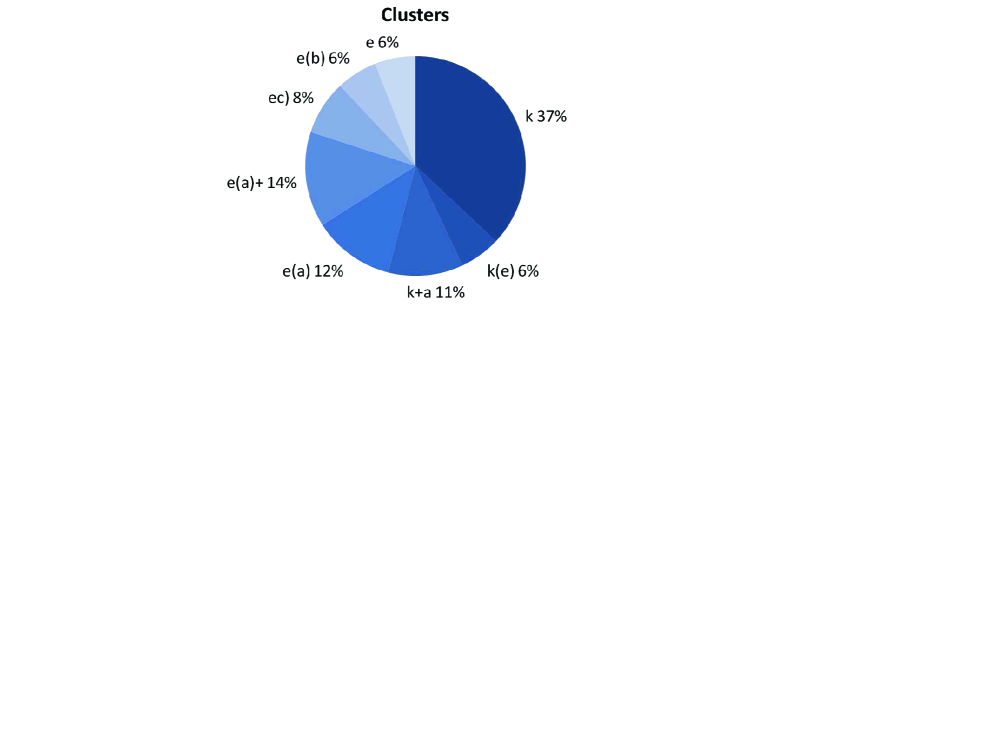
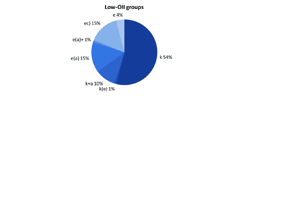
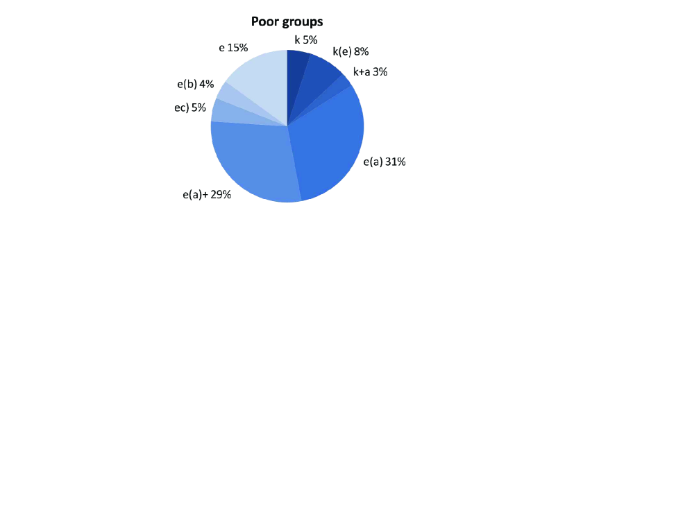
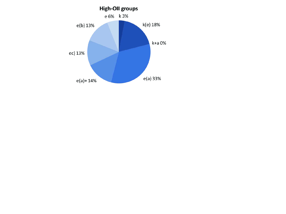
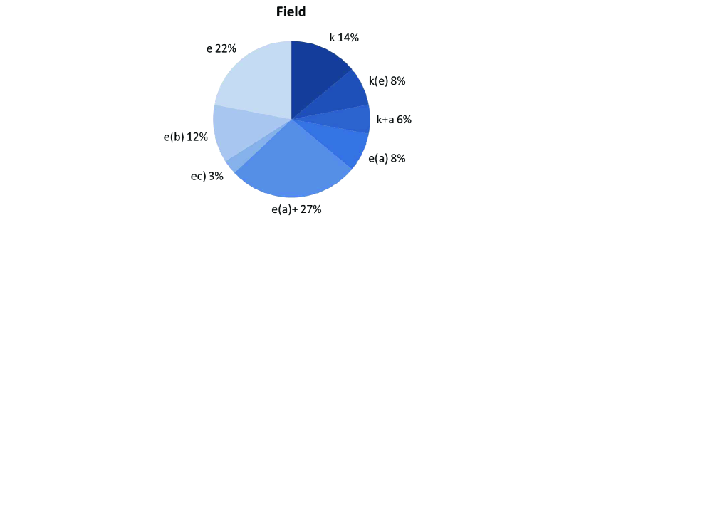
Figure 3.— Graphical representation of the spectral fractions in different environments computed within $R_{200}$ and corrected for spectroscopic incompleteness, as in Table 4.

         

Figure 4.— K+a/active fractions and e(a)/emission fractions in the different environments, as in Table 6.

         

Figure 5.— Fraction of k+a galaxies among the whole cluster population (left) and among the active population (right) versus cluster velocity dispersion. The k+a/active fraction shown in the right panel represents the “quenching efficiency” (see §5.1). Circles are EDisCS structures, outliers in the [OII]-$\sigma$ relation are indicated by empty circles. Stars are MORPHS clusters, MORPHS [OII]-outliers are crosses. The dashed and dotted horizontal lines indicate the poor group and field values, respectively.

         

Figure 6.— Same as Fig. 5, for EDisCS systems grouped in three velocity dispersion bins. The plot shows the total fraction of k+a galaxies among the whole cluster population (left) and among the active population (right) for all systems with $\sigma>750\,\rm km\,s^{-1}$, $400<\sigma<750\,\rm km\,s^{-1}$, and for high-OII (solid leftmost circle) and low-OII (empty circle) groups with $\sigma<400\,\rm km\,s^{-1}$. Only EDisCS structures have been included. The dashed and dotted horizontal lines indicate the poor group and field values, respectively.

         

Figure 7.— Fraction of e(a) galaxies among the whole cluster population (left) and among the active population (right) versus cluster velocity dispersion. Circles are EDisCS structures, outliers in the [OII]-$\sigma$ relation are indicated by empty circles. Stars are MORPHS clusters, MORPHS [OII]-outliers are crosses.

         

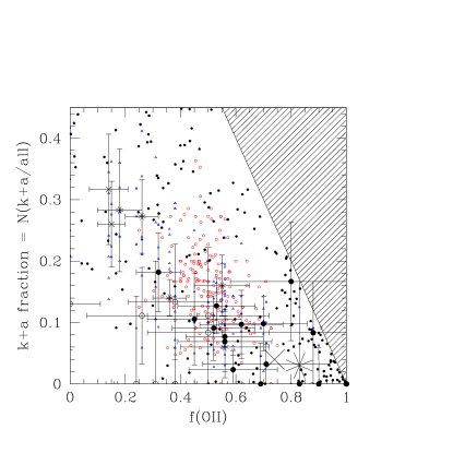
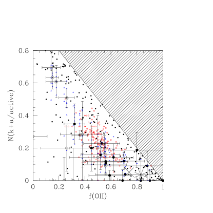
Figure 8.— Fraction of k+a galaxies among the whole cluster population (left) and among the active population (right) versus fraction of [OII] emitters. The large star and cross indicate the poor group and field values, respectively. Other symbols as in Fig.5. The shaded area is the “zone of avoidance” that cannot be populated, given the definition of the X and Y axes (see §5.2). Small black points represent the location of 200 simulated systems with a random f([OII]) and a random k+a fraction (first test in §5.2). Red empty circles are the results for a binomial $f_{OII}$ probability distribution centered around 0.5 and adopting a 30% probability that any one of the non-star-forming galaxies is a k+a (second test in §5.2). Blue empty triangles are the results adopting the observed distribution of $f_{OII}$ and assuming a 30% probability that any one of the non-star-forming galaxies is a k+a (third test in §5.2).

                 

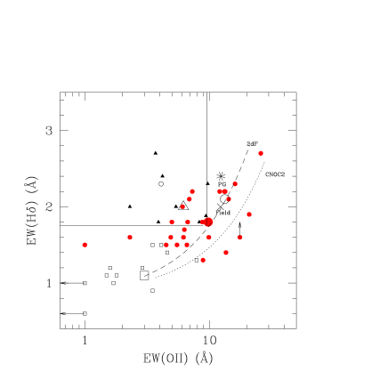
Figure 9.— Rest frame equivalent widths of [OII] and $H\delta$ from composite spectra for 3 datasets of clusters: Dressler & Shectman low redshift clusters as in D04 (empty squares); $z=0.4-0.5$ MORPHS clusters as in D04 (filled triangles) and EDisCS structures at $z=0.4-0.8$ (filled circles). The average of each dataset is indicated by large symbols: empty square for low-z clusters, empty triangle for MORPHS and filled circle for EDisCS. An additional rich cluster at $z\sim 0.8$ (MS1054-03 from D04) is indicated by the small empty circle. The values for EDisCS poor group, field and low-OII group composites are represented by the asterisk, the cross and the large empty circle, respectively. The dashed and dotted lines describe the locus of mixes of passive and continuously star-forming galaxies for low-z (2dF) and $z\sim 0.4$ (CNOC2) field galaxies, respectively, taken from D04. The vertical and horizontal lines are drawn to highlight the region occupied by MORPHS clusters and corresponding to a Balmer excess.

                 

Figure 10.— Morphologies of galaxies of different spectral types. Nonstellar but too compact to see structure = -6, E=-5, S0=-2, Sa=1, Sb=3, Sc=5, Sd=7, Sm=9 Irr=11.

         

Figure 11.— Mass (left), absolute V magnitude (center) and Mass-to-Light ratio (right) distributions of galaxies of different spectral types. The arrows indicate the median value for each type.

                 

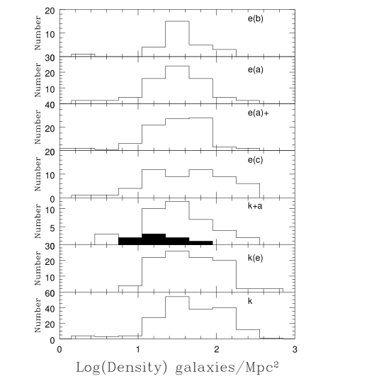
Figure 12.— Projected local density distributions of galaxies of each spectral type. The filled histogram in the k+a panel represent the youngest k+a’s (see text).

                 

Figure 13.— Left Fraction of k+a galaxies among active galaxies (k+a/act) as a function of local density for EDisCS cluster and group galaxies. Solid empty histogram and solid errorbars: all k+a’s. Shaded histogram and dotted errorbars: young k+a’s (see text). Dashed histogram and dashed errorbars: k+a fraction among all galaxies (k+a/all). Errorbars are computed from Poissonian statistics. Right Fraction of e(a) (solid histogram and errorbars), e(c) (dotted histogram and errorbars) and e(b) (dashed histogram and errorbars) galaxies among active galaxies as a function of local density for EDisCS cluster and group galaxies.

                 

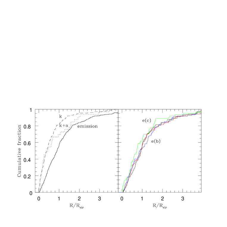
Figure 14.— Radial cumulative distribution of galaxies of different spectral types. Left. K, k+a and all emission line galaxies. Right. Emission line classes: e(a) (black), e(a)+ (red), e(c) (green) and e(b) (blue).

Figure 15.— Composite spectrum of our 6 highest S/N Balmer-strong spectra that cover the $MgII\,2796,2803$ lines. Left For this composite spectrum EW$(H\delta)=4$ Å  and EW(OII)=12 Å. Strong Balmer absorption lines are clearly visible. The arrow indicates the location of the $MgII$ doublet. Right A zoom on the spectral region around the $MgII$ lines. Vertical solid lines indicate the expected line location with no shift. The dotted lines show the shift corresponding to the average velocity found by Tremonti et al. 2007, (1140 $km\,s^{-1}$) at the average redshift of our spectra $z=0.7$.

Appendix A Massive outflows?

Recently, Tremonti et al. (2007) have reported the discovery of massive gas outflows in galaxies with strong Balmer lines in absorption in SDSS spectra at $z\sim 0.6$. Most of these spectra also display an [OII] line in emission, judging from Fig. 1 in Tremonti et al. (2007). Therefore, according to our classification scheme, they would belong to our e(a) class.

Evidence for galactic winds in these galaxies comes from the $MgII2796,2803$ lines that are blueshifted by as much as $\sim 2000km\,s^{-1}$ with respect to the stars. A large mass of outflowing gas can be an efficient method for expelling the galactic gas and terminate the star formation activity. The end of the star formation in this case would be related to a phenomenom intrinsic to the galaxy itself such as an AGN.

184 of our spectra reach sufficiently out in the blue to cover the $MgII2796,2803$ lines. Of these, 31 are cluster members, and of these 13 have spectral characteristics similar to those of Tremonti et al., i.e. have strong Balmer lines in absorption and relatively weak [OII] lines. The great majority of these galaxies belong to our e(a) spectral class, with the exception of 1 k+a. The resemblance of these spectra with those of the galaxies in Tremonti et al. sample can be appreciated comparing our Fig.15 with their Fig. 1.

Measuring the position and strength of the Mg II lines in the spectra of these 13 galaxies, we are able to identify the Mg II lines in most cases and we do not detect significant wavelength shifts in any case. Fig.15 shows the composite spectrum of our 6 best S/N cases, with the strong Balmer absorption lines (EW$(H\delta)$= 4 Å), the relatively weak [OII] (EW=12 Å) and the Mg II lines in place at approximately their rest frame wavelength (right panel in Fig.15).

Moreover, Tremonti et al. (2007) have shown that there is an observed correlation between the outflow velocity $v$ and the galaxy absolute B luminosity in both low-z and high-z samples. Given the moderate typical B luminosity of our small sample ($<M_{B}>=-20.4$), the lack of a blueshift in the Mg II line is consistent with the $v-M_{B}$ correlation.

Thus, we find that galaxies with strong Balmer absorption and weak to moderate emission in our sample do not display signs of galactic winds. Our result shows that this combination of optical spectral features does not need to be generally associated with AGN-powered outflows. The Tremonti et al. galaxies were targeted for SDSS spectroscopy as quasar candidates, though they were subsequently classified as galaxies. Selection criteria other than the strength of $\rm H\delta$ and [OII] must play a role for identifying galaxies with galactic winds.

References

- (1) Abraham, R.G., Smecker-Hane, T.A., Hutchings, J.B., Carlberg, R.G., Yee, H.K.C., Ellingson, E., Morris, S., Oke, J.B., Rigler, M., 1996, ApJ, 471, 694
- (2) Balogh, M.L., Morris, S.L., Yee, H.K.C., Carlberg, R.G., Ellingson, E., 1999, ApJ, 527, 54
- (3) Balogh, M.L., Miller, C., Nichol, R., Zabludoff, A., Goto, T., 2005, MNRAS, 360, 587
- (4) Barger, A. J., Aragón-Salamanca, A., Ellis, R. S., Couch, W. J., Smail, I., & Sharples, R. M. 1996, MNRAS, 279, 1
- (5) Bekki, K., Shioya, Y., Couch, W.J., 2001, ApJ, 547, L17
- (6) Bell, E.F., Zheng, X.Z., Papovich, C., Borch, A., Wolf, C., Meisenheimer, K., 2007, ApJ, 663, 834
- (7) Birnboim, Y., Dekel, A., Neistein, E., 2007, MNRAS, 380, 339
- (8) Biviano, A., Murante, G., Borgani, S., Diaferio, A., Dolag, K., Girardi, M., 2006, A&A, 456, 23
- (9) Blake, C. et al. 2004, MNRAS, 355, 713
- (10) Boselli, A., gavazzi, G., 2006, PASP, 118, 517
- (11) Butcher, A. & Oemler, A., 1984, ApJ, 285, 426
- (12) Caldwell, N., Rose, J.A., Sharples, R.M., Ellis, R.S., Bower, R.G., 1993, AJ, 106, 473
- (13) Clowe, D., et al., 2006, A&A, 451, 395
- (14) Couch, W. J., & Sharples, R. M. 1987, MNRAS, 229, 423
- (15) Crowl, H.H., Kenney, J.D.P., 2006, ApJ, 649, L75
- (16) Desai, V., et al., 2007, ApJ, 660, 1151
- (17) Doherty, M., Bunker, A.J., Ellis, R.S., McCarthy, P.J., 2005, MNRAS, 361, 525
- (18) Douglas, L.S., Bremer, M.N., Stanway, E., Lehnert, M., 2007, MNRAS, 376, 1393
- (19) Dressler, A. & Gunn, J., 1983, ApJ, 270, 7
- (20) Dressler, A. & Gunn, J., 1992 ApJS, 78, 1
- (21) Dressler, A., Smail, I., Poggianti, B. M., Butcher, H., Couch, W. J., et al. 1999, ApJS, 122, 51
- (22) Dressler, A., Oemler, A., Poggianti, B.M., Smail, I., et al., 2004, ApJ, 617, 867
- (23) Dressler, A., Rigby, J., Oemler, A., Fritz, J., Poggianti, B.M., Rieke, G., Bai, L., 2008, ApJ, submitted
- (24) Duc, P.-A., Poggianti, B.M., fadda, D., Elbaz, D., Flores, H., Chanial, P., Franceschini, A., Moorwood, A., Cesarsky, C., 2002, A&A, 382, 60
- (25) Fabricant, D.G., McClintock, J.E., Bautz, M.W., 1991, ApJ, 381, 33
- (26) Finn, R.A., Zaritsky, D., McCarthy, D.W., Poggianti, B.M., Rudnick, G., Halliday, C., Milvang-Jensen, B., Pello, R., Simard, L., 2005, ApJ, 630, 206
- (27) Fritz et al., 2007, A&A, 470, 137
- (28) Gonzalez, A.H., Zaritsky, D., Dalcanton, J.J., Nelson, A., 2001, ApJS, 137, 117
- (29) Goto, T. 2005, MNRAS, 357, 937
- (30) Goto, T. 2007, MNRAS, 381, 187
- (31) Gunn, J.E., Gott, J.R., 1972, ApJ, 176, 1
- (32) Halliday, C. et al., 2004, A&A, 427, 397
- (33) Henry, J.P., Lavery, R.J., 1987, ApJ, 323, 473
- (34) Hogg, D.W., Masjedi, M., berlind, A.A., Blanton, M.R., Quintero, A.D., Brinkmann, J., 2006, ApJ, 650, 763
- (35) Jeltema, T.E., Mulchaey, J.S., Lubin, L.M., Fassnacht, C.D., 2007, ApJ, 658, 865
- (36) Johnson, O. et al., 2006, MNRAS, 371, 1777
- (37) Kapferer, W., Kronberger, T., ferrari, C., Riser, T., Schindler, S., 2008, MNRAS, 389, 1405
- (38) Kaviraj, S., Kirkby, L.A., Silk, J., Sarzi, M., 2007, MNRAS, 382, 960
- (39) Kenney, J.D.P., van Gorkom, J.H., Vollmer, B., 2004, AJ, 127, 3361
- (40) Koopmann, R.A., Kenney, J.D.P., 2004, ApJ, 613, 866
- (41) Lane, K. P., Gray, M. E., Aragón-Salamanca, A., Wolf, C., & Meisenheimer, K. 2007, MNRAS, 378, 716
- (42) Le Borgne, D., et al., 2006, ApJ, 642, 48
- (43) Leonardi, A.J., Rose, J.A., 1996, AJ, 111, 182
- (44) Liu, C.T., Kennicutt, R., 1995, 450, 547
- (45) Ma, C.-J., Ebeling, H., Donovan, D., Barrett, E., 2008, ApJ, accepted (arXiv: 0805.2238)
- (46) Milvang-Jensen, B., et al., 2008, A&A, 482, 419
- (47) Moore, B., Katz, N., Lake, G., Dressler, A., Oemler, A., 1996, Nature, 379, 613
- (48) Moore, B., Lake, G., Quinn, T., Stadel, J., 1999, MNRAS, 304, 465
- (49) Moran, S.M., Ellis, R.S., Treu, T., Smail, I, Dressler, A., Coil, A.L., Smith, G.P., 2005, ApJ, 634, 977
- (50) Moran, S.M., Ellis, R.S., Treu, T., Smith, G.P., Rich, R.M., Smail, I, 2007, ApJ, 671, 1503
- (51) Mulchaey, J.S., Davis, D.S., Mushotzky, R.F., Burstein, D., 2003, ApJS, 145, 39
- (52) Newberry, M.V., Boroson, T.A., Kirshner, R.P., 1990, ApJ, 350, 585
- (53) Nolan, L.A., Raychaudhury, S., Kaban, A., 2007, MNRAS, 375, 381
- (54) Norton, S.A., Gabhardt, K., Zabludoff, A.I., Zaritsky, D., 2001, ApJ, 557, 150
- (55) Oemler, A., Dressler, A., Kelson, D.D., Rigby, J., Poggianti, B.M., Fritz, J., Morrison, G., Smail, I., 2008, ApJ, submitted
- (56) Osmond, J.P.F., Ponman, T.J., 2004, MNRAS, 350, 1511
- (57) Pelló R. et al., 2008, A&A submitted
- (58) Poggianti, B.M., Barbaro, G., 1996, A&A, 314, 379
- (59) Poggianti, B.M., Barbaro, G., 1997, A&A, 325, 1025
- (60) Poggianti, B.M., Wu, H., 2000, ApJ, 529, 157
- (61) Poggianti, B.M., Bressan, A., Franceschini, A., 2001, ApJ, 550, 195
- (62) Poggianti, B. M., Smail, I., Dressler, A., Couch, W. J., Barger, A. J., Butcher, H., et al. 1999, ApJ, 518, 576
- (63) Poggianti, B.M., 2004 in Clusters of Galaxies: Probes of Cosmological Structure and Galaxy Evolution, edited by J.S. Mulchaey, A. Dressler, and A. Oemler, p. 245.
- (64) Poggianti, B.M., Bridges, T.J., Komiyama, Y. et al., 2004, ApJ, 601, 197
- (65) Poggianti, B.M., et al., 2006, ApJ, 642, 188
- (66) Poggianti et al., 2008, ApJ, in press, arXiv: 0805.1145
- (67) Rawlings, S., Jarvis, M.J., 2004, MNRAS, 355, L9
- (68) Sanchez-Blazquez, P. et al., 2008, A&A in prep.
- (69) Shioya, Y, bekki, K., Couch, W.J., 2001, ApJ, 558, 42
- (70) Smail, I., Morrison, G., Gray, M.E., Owen, F.N., Ivison, R.J., kneib, J.-P., Ellis, R.S., 1999, ApJ, 525, 609
- (71) Swinbank, A.M., Edge, A.C., Smail, I., et al;., 2007, MNRAS, 379, 1343
- (72) Tonnesen, S., Bryan, G.L., van Gorkom, J.H., 2007, ApJ, 671, 1434
- (73) Tonnesen, S., Bryan, G.L., 2008, ApJ, 684, L9
- (74) Tran, K.-V. H., Franx, M., Illingworth, G., Kelson, D. D., van Dokkum, P., 2003, ApJ, 599, 865
- (75) Tran, K.-V., Franx, M., Illingworth, G.D., van Dokkum, P., Kelson, D.D., Magee, D., 2004, ApJ, 609, 683
- (76) Tran, K.-V. H., Franx, M., Illingworth, G.D., van Dokkum, P., Kelson, D.D., Blakeslee, J.P., Postman, M., 2007, ApJ, 661, 750
- (77) Tremonti, C.A., Moustakas, J., Diamond-Stanic, A.M., 2007 ApJL 663 L77
- (78) Treu, T., Ellis, R.S., Kneib, J.-P., Dressler, A., Smail, I., Czoske, O., Oemler, A., Natarajan, P., 2003, ApJ, 591, 53
- (79) van Dokkum, P.G., Ellis, R.S., 2003, ApJ, 592, L53
- (80) van Dokkum, P.G., Stanford, S.A., 2003, ApJ, 585, 78
- (81) Vollmer, B., Soida, M., Otmianowska-Mazur, K., Kenney, J.D.P., van Gorkom, J.H., Beck, R., 2006, A&A, 453, 883
- (82) Vollmer, B., 2008, in Mapping the galaxy and nearby galaxies, Astrophysics and Space Science Proceedings, p.253
- (83) Yamauchi, C., Yagi, M., Goto, T., 2008, MNRAS, in press arXiv: 0809.0890
- (84) Yan, R., Newman, J.A., Faber, S.M.,. Konidaris, N., Koo, D., Davis, M., 2006, ApJ, 648, 281
- (85) Yan, R., Newman, J.A., Faber, S.M., Coil, A.L., Cooper, M.C., Davis, M., Weiner, B.J., Gerke, B.F., Koo, D.C., 2008, MNRAS, submitted arXiv: 0805.0004
- (86) Yang, Y., Zabludoff, A., Zaritsky, D., lauer, T.R.., Mihos, C., 2004, ApJ, 607, 258
- (87) Yang, Y., Zabludoff, A., Zaritsky, D., Mihos, C., 2008, ApJ, submitted arXiv: 0801.1190
- (88) White et al., 2005, A&A, 444, 365
- (89) Wolf, C., Gray, M. E., & Meisenheimer, K. 2005, A&A, 443, 435
- (90) Wolf, C., et al., 2007, American Astronomical Society, AAS Meeting 211, 67.01
- (91) Zabludoff, A.I., Zaritsky, D., Lin, H., Tucker, D., Hashimoto, Y., Shectman, S.A., Oemler, A., Kirshner, R.P.., et al. 1996, ApJ, 466, 104
- (92) Zabludoff, A.I., Mulchaey, J.S., 1998, ApJ, 496, 39