Abstract

The dispersion of index-guiding microstructured polymer optical fibers is calculated for second-harmonic generation. The quadratic nonlinearity is assumed to come from poling of the polymer, which in this study is chosen to be the cyclic olefin copolymer Topas. We found a very large phase mismatch between the pump and the second-harmonic waves. Therefore the potential for cascaded quadratic second-harmonic generation is investigated in particular for soliton compression of fs pulses. We found that excitation of temporal solitons from cascaded quadratic nonlinearities requires an effective quadratic nonlinearity of 5 pm/V or more. This might be reduced if a polymer with a low Kerr nonlinear refractive index is used. We also found that the group-velocity mismatch could be minimized if the design parameters of the microstructured fiber are chosen so the relative hole size is large and the hole pitch is on the order of the pump wavelength. Almost all design-parameter combinations resulted in cascaded effects in the stationary regime, where efficient and clean soliton compression can be found. We therefore did not see any benefit from choosing a fiber design where the group-velocity mismatch was minimized. Instead numerical simulations showed excellent compression of $\lambda=800$ nm 120 fs pulses with nJ pulse energy to few-cycle duration using a standard endlessly single-mode design with a relative hole size of 0.4.

OCIS codes:  060.4005, 190.4370, 320.5520, 320.7110, 320.2250, 190.5530, 190.2620

1 Introduction

Microstructured optical fibers allows for an elaborate dispersion control. Usually they are exploited to gain control over the group-velocity dispersion (GVD) [1] (see [2] for a recent literature overview over the dispersion properties of microstructured optical fibers). Also the group-velocity mismatch (GVM) for three-wave mixing processes can be completely removed [3], which is important in order to realize second-harmonic generation (SHG) of ultra-short fs pulses. However, the prize for having a small GVM is that the phase mismatch becomes very large [3], and efficient SHG would therefore rely on quasi-phase matching (QPM) techniques.

The large phase-mismatch $\Delta\beta$ can instead be exploited for cascaded $\chi^{(2)}:\chi^{(2)}$ SHG processes [4]. The second harmonic (SH) is within a coherence length $2\pi/|\Delta\beta|$ generated and then back-converted to the fundamental wave (FW). This cascaded process generates a nonlinear phase shift $\Phi_{\rm NL}$ on the FW [5], which can become several units of $\pi$ by propagating in just a few cm’s of nonlinear material, and is conceptually equivalent to the nonlinear phase shift observed through self-phase modulation (SPM) with cubic nonlinearities [6].

The large nonlinear phase shift can be exploited to compress ultra-short fs pulses [7]. This is particularly advantageous when the compression occurs inside the nonlinear material due to the soliton effect [8, 9]; the cascaded SHG process can generate a negative $\Phi_{\rm NL}$ resulting in a negatively chirped FW, and if the material has normal GVD a temporal soliton is generated. By launching a higher-order soliton, the input pulse can be compressed by exploiting the initial pulse narrowing. This cascaded quadratic soliton compressor (CQSC) can in principle compress the FW pulse to single-cycle duration, and is ultimately limited by higher-order dispersion and competing Kerr nonlinear effects [10].

One requirement for efficient compression is that GVM effects are not too strong: they tend to distort the compressed pulses through a Raman-like effect [11, 9, 12, 10]. In fact, when GVM dominates over the cascaded effects from the phase mismatch the compression is nonstationary, resulting in inefficient compression and distorted pulses. Therefore the possibility offered by microstructured optical fibers to control GVM is very intriguing for the CQSC, because the compression can become stationary, which implies efficient compression and clean pulses. The fiber geometry can also help overcoming the problem of inhomogeneous compression in the transverse direction of the beam found in a bulk geometry [13].

We have done a preliminary investigation of the potential in using silica microstructured optical fibers for CQSC [14, 2], where the quadratic nonlinearity was assumed to come from thermal poling of the silica fiber [15]. We surprisingly found that zero GVM was not as such an advantage, since the compressed pulses became very distorted. Another main result was that a very large quadratic nonlinearity $d_{\rm eff}\sim 3-5$ pm/V was needed in order to generate suitably large $\Phi_{\rm NL}$ [2]. This is because the chosen fiber designs had very a large phase mismatch, and $\Phi_{\rm NL}\propto d_{\rm eff}^{2}/\Delta\beta$. Realistically, thermal poling of silica fibers can generate $d_{\rm eff}\sim 0.5$ pm/V [16]. Therefore we suggested to lower the phase mismatch using QPM techniques, and in this way a much lower $d_{\rm eff}\sim 1$ pm/V was sufficient [14]. However, periodic thermal poling of silica fibers have until now proved inefficient, and has resulted in a much lower $d_{\rm eff}\sim 0.01$ pm/V than expected [17]. We must therefore conclude that periodically poled silica (microstructured) fibers cannot generate large enough $\Phi_{\rm NL}$ to be interesting for CQSC.

A large $d_{\rm eff}$ would compensate for a large $\Delta\beta$. In this paper, we therefore turn our attention to microstructured polymer optical fibers (mPOFs). Poling of polymers can generate extremely large quadratic nonlinearities (ranging from 1 pm/V to 100’s of pm/V) [18], while poling still has to be shown in a fiber context. Alternatively, the low mPOF drawing temperature (few hundred degrees C) implies that nanomaterials with large quadratic nonlinear responses (such as nanotubes [19]) can be drawn into the fiber core. Also this solution promises a strong $d_{\rm eff}$. The potential for using mPOFs for quadratic nonlinear optics is therefore large.

Here we calculate the dispersion properties of an index-guiding mPOF with three rings of air-holes in the cladding. The polymer material is chosen to be the cyclic olefin copolymer Topas due to its broad transparency window [20]. We point out that a problem with using polymer as fiber material is that unlike silica the material Kerr nonlinearity is very large, and it generates an SPM-induced positive nonlinear phase shift which has to be overcome by the negative cascaded nonlinear phase shift. We will show that for the considered polymer Topas $d_{\rm eff}>5$ pm/V is needed to do so (compared to $d_{\rm eff}\sim 3-5$ pm/V in silica [14, 2]). Such a value could be achieved with polymers as fiber material. We also show that the fiber designs with a dramatically reduced GVM are multi-moded in the SH, and thus one risks to have cascaded nonlinear conversion to several SH modes. Quite surprisingly we find that the compression is always in the stationary regime, irrespective of the choice of fiber-design parameters. This is very positive since efficient and clean compression can be obtained. On the other hand, there is no longer any motivation for reducing GVM in order to enter the stationary regime. Thus, we conclude that there are very few benefits of reducing GVM through fiber design. This statement is underlined by performing numerical simulations of the propagation equations for an mPOF having $d_{\rm eff}=10$ pm/V: an endlessly single-moded mPOF design dominated mainly by material dispersion turns out to give clean and efficient compression of fs pulses, and obtaining compressed pulses with durations close to single-cycle duration is possible. So if the potentially large $d_{\rm eff}$ of polymer material can be exploited, then excellent pulse compression can be obtained in mPOFs.

2 Nonlocal theory

The scope of this theoretical part is to point out the important parameters when choosing the proper fiber design. The main hypothesis is that an mPOF can be used as a CQSC. The challenges with creating a quadratic nonlinearity in the fiber aside, there are other obstacles that must be faced. Understanding these issues can be greatly enhanced by realizing that in the cascading regime, the coupled FW and SH propagation equations reduce to a nonlinear Schrödinger equation (NLSE) for the FW [6]. The action of the cascaded SHG can be modeled as a Kerr-like nonlinearity with an equivalent nonlinear refractive index $n_{\rm SHG}^{I}\propto d_{\rm eff}^{2}/\Delta\beta$. Importantly, when $\Delta\beta=\beta_{2}-2\beta_{1}>0$ (which is usually the case) $n_{\rm SHG}^{I}$ is self-defocusing of nature: it generates a negative nonlinear phase shift $\Phi_{\rm NL}<0$. The material Kerr nonlinear refractive index $n_{\rm Kerr}^{I}$ is instead usually self-focusing, and therefore counteracts the effects of the cascaded nonlinearities. Achieving $n_{\rm SHG}^{I}>n_{\rm Kerr}^{I}$ is crucial to obtain a large negative nonlinear phase shift. An important point here is that because the cascaded SHG induces a self-defocusing Kerr-like nonlinearity, temporal solitons exists in presence of normal GVD. In contrast, the usual cubic temporal solitons observed for instance in telecom fibers require anomalous GVD due to the self-focusing Kerr nonlinearity of silica [21].

GVM is also playing a decisive role. As we recently showed, the pulse compression is clean and efficient in the stationary regime, where the phase mismatch dominates over GVM effects [12, 10]. These results were obtained by deriving a more general NLSE, where dispersion including GVM imposes a Raman-like nonlocal (delayed) temporal cubic nonlinearity. Contrary to earlier reports [7, 11] we showed that the regime where efficient compression takes place is independent on the input pulse duration.

In the remainder of this section we briefly show how the nonlocal NLSE for the FW is derived, and discuss the consequences for soliton pulse compression. The equation is derived in dimensionless form based on the SHG propagation equations derived in App. A.

The nonlocal theory was derived in Refs. [12, 10] (for a general review on nonlocal effects, see [22]). Essentially in the cascading limit (large phase mismatch), the SH becomes slaved to the FW. The normalized FW $U_{1}$ can then on dimensionless form be modeled by the following nonlocal nonlinear Schrödinger equation (NLSE) [12]

$$\left[i\frac{\partial}{\partial\xi}-\frac{{\rm sgn}(\beta^{(2)}_{1})}{2}\frac{\partial^{2}}{\partial\tau^{2}}\right]U_{1}+N_{\rm Kerr}^{2}U_{1}|U_{1}|^{2}$$ (1)

$$=N_{\rm SHG}^{2}U_{1}^{*}\int_{-\infty}^{\infty}{\rm d}sR_{\pm}(s)U_{1}^{2}(\xi,\tau-s).$$

where Kerr cross-phase modulation (XPM) effects have been neglected, and for simplicity self-steepening and higher-order dispersion are not considered. On the left-hand side an ordinary NLSE appears with an SPM-term from self-focusing material Kerr nonlinearities. On the right-hand side the effects of the cascaded SHG appear: it is also SPM-like in nature, but it turns out to be controlled by a temporal nonlocal response. The dimensionless temporal nonlocal response function $R_{\pm}(\tau)$ appears in two distinct ways: in the stationary regime it is given by $R_{+}$, and $|R_{+}|\propto e^{-|\tau|/\tau_{b}}$ is localized having a characteristic width $\tau_{b}$ of a few fs. This happens when the phase mismatch is dominating over GVM effects, or more precisely when $\Delta\beta>\Delta\beta_{\rm sr}$, with

$$\Delta\beta_{\rm sr}=\frac{d_{12}^{2}}{2\beta^{(2)}_{2}}=-\frac{\pi d_{12}^{2}}{{\mathcal{D}}_{2}\lambda_{2}^{2}}.$$ (2)

and ${\mathcal{D}}_{2}=-2\pi\beta^{(2)}_{2}/\lambda_{2}^{2}$ is the fiber GVD parameter. In the stationary regime clean and efficient compression can be obtained [9, 12, 23, 10]. Instead in the nonstationary regime ($\Delta\beta<\Delta\beta_{\rm sr}$) GVM effects dominate, and the compression becomes distorted and inefficient. In this case the nonlocal response function is given by $R_{-}$, and $|R_{-}|\propto\sin(|\tau|/\tau_{b})$ is oscillatory and never decays.

The fiber designs presented here all turn out to be in the stationary regime. In this case, and when the nonlocal response function can be assumed quasi-instantaneous, Eq. (1) can be written as [11, 9, 12]

$$\left[i\frac{\partial}{\partial\xi}-\frac{{\rm sgn}(\beta^{(2)}_{1})}{2}\frac{\partial^{2}}{\partial\tau^{2}}\right]U_{1}\\ -[{\rm sgn}(\Delta\beta)N_{\rm SHG}^{2}-N_{\rm Kerr}^{2}]U_{1}|U_{1}|^{2}\\ =-iN_{\rm SHG}^{2}s_{a}\tau_{R,\rm SHG}|U_{1}|^{2}\frac{\partial U_{1}}{\partial\tau}$$ (3)

The soliton order for the Kerr fiber nonlinearity is [24]

$$N_{\rm Kerr}^{2}=\frac{L_{\rm D,1}}{L_{\rm Kerr}}$$ (4)

where $L_{\rm D,1}=T_{\rm in}^{2}/|\beta^{(2)}_{1}|$ is the characteristic GVD length of the FW, and $L_{\rm Kerr}=(\gamma_{\rm Kerr}P_{\rm in})^{-1}$ is the characteristic Kerr nonlinear length. $P_{\rm in}=\varepsilon_{0}n_{{\rm eff},1}ca_{1}{\mathcal{E}}_{\rm in}^{2}/2$ is the input peak power, related to the peak input electric field ${\mathcal{E}}_{\rm in}$. The Kerr nonlinear coefficient is

$$\gamma_{\rm Kerr}=n_{\rm Kerr}^{I}\frac{\omega_{1}}{cA_{{\rm eff},1}}$$ (5)

where $A_{{\rm eff},1}$ is the effective Kerr FW mode overlap area

$$A_{{\rm eff},1}=\frac{(\int d\mathbf{x}|F_{1}(\mathbf{x})|^{2})^{2}}{\int_{P}d\mathbf{x}|F_{1}(\mathbf{x})|^{4}}$$ (6)

Note that $A_{{\rm eff},1}\equiv f_{11}^{-1}$ from Eq. (23), and that as explained in App. A the subscript ’P’ indicates that integration must be done only over the part of the fiber mode sitting in the polymer part of the mPOF. We also encounter the well-known Kerr nonlinear refractive index $n_{\rm Kerr}^{I}$: the refractive index change due to the Kerr self-focusing effect is defined as $\Delta n=n_{\rm Kerr}^{I}I$, where $I$ is the intensity of the beam. Although it is not known for the Topas polymer, we estimate (based on similar polymer types) that it is in the range $n_{\rm Kerr}^{I}\sim 10-15\cdot 10^{-20}~{}{\rm m^{2}/W}$, which is an order of magnitude larger than for fused silica.

In a similar way we have introduced a soliton order from the cascaded SHG process

$$N_{\rm SHG}^{2}=\frac{L_{\rm D,1}}{L_{\rm SHG}}$$ (7)

where $L_{\rm SHG}=(\gamma_{\rm SHG}P_{\rm in})^{-1}$. Here the nonlinear coefficient is defined as for the Kerr case

$$\gamma_{\rm SHG}=|n_{\rm SHG}^{I}|\frac{\omega_{1}}{cA_{\rm SHG}}$$ (8)

only it contains the SHG overlap area $A_{\rm SHG}$

$$A_{\rm SHG}=\frac{a_{1}^{2}a_{2}}{|\int_{P}d\mathbf{x}[F_{1}^{*}(\mathbf{x})]^{2}F_{2}(\mathbf{x})|^{2}}$$ (9)

where $a_{j}$ are the fiber mode areas (19). The “effective” nonlinear refractive index from the cascaded process [5]

$$n_{\rm SHG}^{I}=-\frac{4\pi d_{\rm eff}^{2}}{c\varepsilon_{0}\lambda n_{{\rm eff},1}^{2}n_{{\rm eff},2}\Delta\beta}$$ (10)

Note the negative sign in front of $n_{\rm SHG}^{I}$; since the cases we will discuss always have $\Delta\beta>0$ the cascaded nonlinearity is therefore self-defocusing. Thus, in order to generate a negative nonlinear phase shift we must have $\gamma_{\rm SHG}>\gamma_{\rm Kerr}$. We can express this through an effective soliton order

$$N_{\rm eff}^{2}=N_{\rm SHG}^{2}-N_{\rm Kerr}^{2}=P_{\rm in}L_{\rm D,1}\left(\gamma_{\rm SHG}-\gamma_{\rm Kerr}\right)$$ (11)

Using this in Eq. (3) we then get an NLSE with a self-defocusing SPM term:

$$\left[i\frac{\partial}{\partial\xi}-\frac{1}{2}\frac{\partial^{2}}{\partial\tau^{2}}\right]U_{1}-N_{\rm eff}^{2}U_{1}|U_{1}|^{2}\\ =-iN_{\rm SHG}^{2}s_{a}\tau_{R,\rm SHG}|U_{1}|^{2}\frac{\partial U_{1}}{\partial\tau}$$ (12)

Self-defocusing solitons with strength $N_{\rm eff}^{2}$ can then be excited if the FW GVD is normal, i.e. if $\beta^{(2)}_{1}>0$, which has been taken into account in Eq. (12).

So the LHS of Eq. (12) is now a self-defocusing NLSE supporting solitons if $N_{\rm eff}\geq 1$. The RHS contains the Raman-like perturbation due to GVM. It becomes important for large SHG soliton orders $N_{\rm SHG}$ [10] and when the compressed pulse duration is on the order of $T_{R,\rm SHG}=\tau_{R,\rm SHG}T_{\rm in}$, where the characteristic dimensionless time scale of the Raman-like perturbation is

$$\tau_{R,\rm SHG}\equiv\frac{2|d_{12}|}{\Delta\beta T_{\rm in}}$$ (13)

Typically $T_{R,\rm SHG}$ is on the order of 1-5 fs, but can become very large in the nonstationary regime [10]. Finally, $s_{a}={\rm sgn}(d_{12}\beta^{(2)}_{2})$: the Raman-like effect will depending on this sign give either a red-shifting ($s_{a}=+1$) or blue-shifting ($s_{a}=-1$) of the FW spectrum. In the cases we present here $s_{a}=-1$.

3 Numerical results

In this section the transverse fiber modes and their dispersion properties are calculated for various mPOF designs (varying the air-hole diameter $d$ and the hole pitch $\Lambda$). Then we show compression examples for selected fiber designs. These numerical simulations were done using the full coupled propagation equations (22), which include Kerr XPM effects, steepening terms, and are valid down to single-cycle resolution using the slowly-evolving wave approximation [25, 26, 23].

A The microstructured fiber

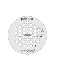
Fig. 1: The microstructured fiber design considered here.

We consider an index-guiding mPOF with a triangular air-hole pattern in the cladding, see Fig. 1. The mPOF design parameters are the pitch $\Lambda$ between the air holes and the relative air hole size $D=d/\Lambda$, where $d$ is the physical air-hole diameter. We assume that the core has a quadratic nonlinearity from thermal poling of the polymer after the fiber drawing, or from including nonlinear nanomaterial in the fiber preform.

We consider an mPOF made from the cyclic olefin copolymer Topas [20]. The advantage of using Topas compared to, e.g., poly-(methyl methacrylate) (PMMA), is that Topas has a larger transparency window: it is transparent from 300-1700 nm, interrupted by two absorption peaks around 1200 nm and 1450 nm [20], see App. C for more details.

B Fiber design, dispersion and compression

We will here search for fiber design parameters, where the requirement is an optimal dispersion profile for cascaded quadratic soliton compression. Details about the fiber mode calculations and the dispersion calculations are found in App. B.

Two types of designs are discussed: one is a realistic mPOF with a large air-hole pitch of around $\Lambda=7~{}{\rm\mu m}$ that can easily be drawn, while another takes $\Lambda$ small (comparable to the FW wavelength) as to significantly alter the dispersion parameters. Such an mPOF would probably need to be done by tapering an mPOF with a larger pitch. In the calculations the Sellmeier equation from App. C with $T=25^{\circ}$C was used.

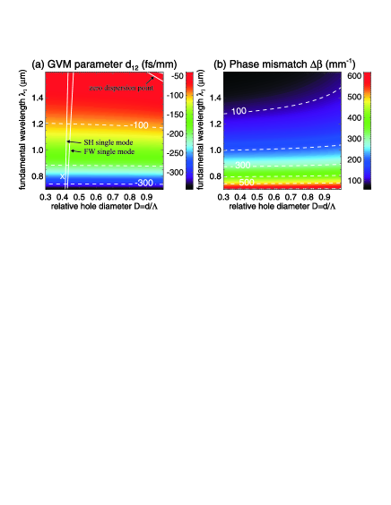
Fig. 2: The GVM parameter $d_{12}$ and phase mismatch $\Delta\beta$ for an mPOF with $\Lambda=7.0~{}{\rm\mu m}$. In (a) the lines for single-mode operation are indicated for the FW and the SH modes. The FW zero dispersion point is also indicated; below this line the FW GVD is normal. Finally the ’X’ indicates the chosen fiber design for single-mode operation at $\lambda_{1}=800$ nm.

It is fairly standard to draw mPOFs with a air-hole pith of $\Lambda>5~{}{\rm\mu m}$. With this as a starting point we show in Fig. 2 the GVM and phase mismatch for a Topas mPOF with $\Lambda=7.0~{}{\rm\mu m}$. We notice that the choice of $D$ does not affect the dispersion parameters much. This is because the size of the waveguide [the core diameter is $d_{\rm core}=\Lambda(2-D)$] is significantly larger than the wavelength of the guided light, and so material dispersion is dominating (see also Fig. 3). The microstructured cladding therefore alters the dispersion only very little, and we cannot get tailored GVM or GVD properties.

Since Topas has a primary transparency window between 290-1210 nm, we focus now on SHG with $\lambda_{1}=800$ nm. We would like the fiber to be single mode both at the FW and at the SH wavelength, because then phase matching can only occur between these modes and we do not have problems with the typical higher-order mode interaction usually observed in wave-guided SHG. The criterion for single-mode operation in the particular microstructured fiber, we investigate, is [27] $\lambda/\Lambda=2.8(D-0.406)^{0.89}$. This criterion gives the lines shown in Fig. 2(a) for the FW (where $\lambda=\lambda_{1}$) and the SH (where $\lambda=\lambda_{2}=\lambda_{1}/2$). We therefore choose a design with $D=0.4$, which is indicated with an ’X’; this design is actually endlessly single-moded [28].

Fig. 3: The dispersion for $\Lambda=7.0~{}{\rm\mu m}$ and $D=d/\Lambda=0.4$. (a) the phase mismatch $\Delta\beta=\beta_{2}-2\beta_{1}$ and (b) GVM $d_{12}=\beta_{1}^{(1)}-\beta_{2}^{(2)}$ vs. $\lambda_{1}$. (c) the GVD parameter ${\mathcal{D}}=-2\pi c\beta^{(2)}/\lambda^{2}$ vs. $\lambda$. The material dispersion is also shown. (d) shows the effective nonlinearity required to achieve $\gamma_{\rm SHG}>\gamma_{\rm Kerr}$ for $n_{\rm Kerr}^{I}=15\cdot 10^{-20}~{}{\rm m^{2}/W}$.

For the chosen design, we show in Fig. 3 the dispersion parameters as function of wavelength. In (a) the phase mismatch $\Delta\beta$ is shown. It is always above the boundary to the stationary regime as given by Eq. (2) $\Delta\beta_{\rm sr}=d_{12}^{2}/2\beta_{2}^{(2)}$. Thus, the chosen fiber design for all the shown wavelengths is in the stationary regime for soliton compression, which is very good news for the possibility of clean and efficient compression. This might seem surprising given the large GVM seem in Fig. 3(b), but it is a consequence of having a very large phase mismatch and the very large GVD at the SH wavelength, see Fig. 3(c). However, the large phase mismatch unfortunately also implies a small cascaded nonlinear parameter $\gamma_{\rm SHG}$. In order to achieve $\gamma_{\rm SHG}>\gamma_{\rm Kerr}$, as required for solitons to exist, the effective quadratic nonlinearity $d_{\rm eff}$ must be quite high, around 6 pm/V for $\lambda_{1}=800$ nm as shown in Fig. 3(d).

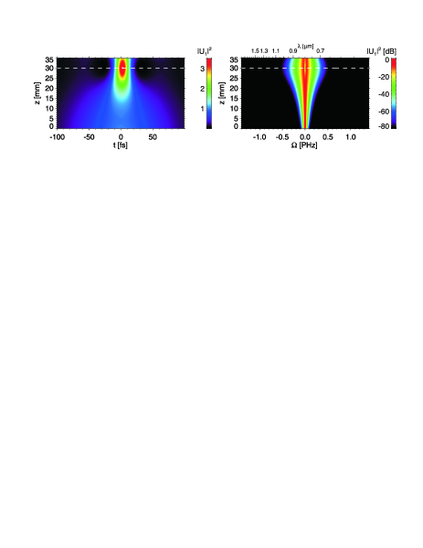
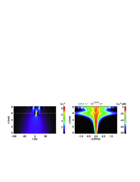
Fig. 4: Numerical simulation of soliton compression in an mPOF with the design parameters of Fig. 3 and $d_{\rm eff}=10$ pm/V. Top left plot shows the FW compressing to 15 fs FWHM after 30 mm of propagation (at the dashed line) starting from 120 fs. Top right shows the spectral broadening and development of SPM-induced sidebands of the FW. The pulse parameters were $N_{\rm eff}=3$, $P_{\rm in}=4.6$ kW, and the pulse energy was 0.6 nJ. The middle row shows a simulation for a higher soliton order ($N_{\rm eff}=9$, $P_{\rm in}=41.8$ kW, and a pulse energy of 5.7 nJ), which compresses to 4.4 fs after 6 mm of propagation. A cut at $z=6$ mm is shown in the bottom plot. Up to 10th order dispersion was included ($m_{d}=10$). $2^{13}$ temporal points and $>15$ $z$-steps per coherence length were used.

In Fig. 4 we show numerical simulations of soliton compression using the chosen design. For the Kerr nonlinear refractive index of the polymer Topas we use $n_{\rm Kerr}^{I}=15\cdot 10^{-20}~{}{\rm m^{2}/W}$, which is a large but realistic value. In order to outbalance this Kerr self-focusing nonlinearity the quadratic nonlinearity must be $d_{\rm eff}>6$ pm/V, see Fig. 3(d), and $d_{\rm eff}=10.0$ pm/V was chosen. The compression is shown for both a low and a high soliton order, and both are very clean for several reasons: firstly, the compression occurs in the stationary regime, and secondly the Raman-like perturbation is very small, $T_{R,\rm SHG}=1.3$ fs. Lastly, looking at the FW frequency spectra there are no dispersive waves. These tend to induce trailing oscillations on the compressed pulse [10], but we checked that for this fiber design they are not phase matched in the transparent region of Topas. We should also mention that we have neglected any cubic Raman effects of the material due to the lack of material knowledge in this respect, and if significant Raman effects are present as for silica fibers then this would have an impact on the results.

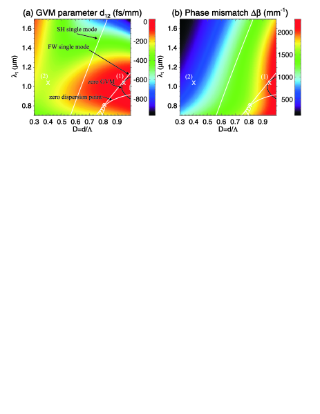
Fig. 5: As Fig. 2 but with $\Lambda=0.65~{}{\rm\mu m}$. A zero GVM curve is indicated with black as well as the FW zero dispersion point (ZDP). The two ’X’es indicates the chosen fiber designs at $\lambda_{1}=1040$ nm.

So a standard mPOF, where the fiber simply serves as a waveguide but otherwise has little influence on the dispersion, can give decent compression (provided $d_{\rm eff}$ is high enough). What benefits can we get with a reduced GVM? To get a detailed understanding of this, let us investigate a possible fiber design having very small GVM.

In order to significantly alter the dispersion, the mPOF must have a lower hole pitch. As an extreme example Fig. 5 shows the calculated fiber properties for $\Lambda=0.65~{}{\rm\mu m}$ : the GVM can be very small or even zero along the black curve. Unfortunately for $\lambda_{1}=800$ nm this low-GVM area is in an anomalous dispersion region, where cascaded solitons do not exist, so let us instead work at $\lambda_{1}=1040$ nm, which would be relevant for compressing the output of Yb:doped fiber lasers.

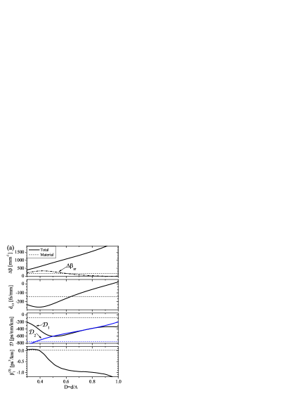
Fig. 6: (a) The dispersion as function of the relative hole size $D$ as calculated for $\lambda_{1}=1040$ nm and $\Lambda=0.65~{}{\rm\mu m}$. (b) The the effective nonlinearity required to achieve $\gamma_{\rm SHG}>\gamma_{\rm Kerr}$ assuming $n_{\rm Kerr}^{I}=15\cdot 10^{-20}~{}{\rm m^{2}/W}$.

The dispersion for $\lambda_{1}=1040$ nm of this mPOF with $\Lambda=0.65~{}{\rm\mu m}$ is shown in Fig. 6(a) as function of $D$. Clearly the dispersion changes dramatically as $D$ is changed. The GVM goes from a normal value ($d_{12}\sim-200$ fs/mm) for low $D$ to zero at high $D$. Nonetheless, we remain in the stationary regime even for low $D$-values since $\Delta\beta>\Delta\beta_{\rm sr}$ always. This is because both $\Delta\beta$ and the SH GVD ${\mathcal{D}}_{2}$ are large. Notice also that the FW third order dispersion $\beta_{1}^{(3)}$ changes dramatically: it is very large for high $D$ and close to zero for low $D$. Finally, Fig. 6(b) shows the critical $d_{\rm eff}$ required in order to overcome the material Kerr self-focusing effects. It is around 2-3 times higher than in Fig. 3, which is a consequence of a large $\Delta\beta$.

Zero GVM can therefore be achieved choosing $D=0.95$ [at the cross marked (1) in Fig. 5]. This choice leaves the SH multi-moded, and is therefore not suitable for compression: there would be different modes with different degrees of phase mismatch interacting with the FW, and gaining control over the compression would be difficult. If we want the SH to be single moded, we should choose a design below $D=0.6$ (see Fig. 5), and the design marked with ’X’ (2) in Fig. 5 has the advantage of being endlessly single moded. In this regime the GVM is not too different from material dispersion.

So the penalty of choosing a small-pitched fiber in order to reduce the GVM seems to be too high. The main motivation behind controlling GVM through the fiber microstructure was to be in the stationary regime. However, almost all mPOF designs we have investigated have been in the stationary regime thanks to the large phase mismatch. Another motivation was to reduce the characteristic time of the Raman-like response $T_{R,\rm SHG}=|d_{12}|/2\Delta\beta$ as to get cleaner compressed pulses, but $T_{R,\rm SHG}$ is low even when GVM is not reduced again thanks to the large phase mismatch. What is more, choosing a zero GVM design surprisingly has been shown not to benefit compression: In our previous study [14] we performed simulations with just the lowest SH transverse mode (neglecting the higher-order modes), and the fiber designs with zero GVM were giving quite distorted compressed pulses. This can be partially explained by the fact that higher-order dispersion is significant when the relative hole size is large; observe for instance how large the third-order dispersion is in Fig. 6 for $D$ close to unity: this value is several order of magnitude stronger than the material third-order dispersion.

Fig. 7: The dispersion calculated for $D=0.4$ nm and $\Lambda=1.0~{}{\rm\mu m}$. The lower plot shows the results of a numerical simulation, where a $\lambda_{1}=800$ nm $T_{\rm in}=120$ fs FWHM input pulse is compressed to 5.5 fs. The pulse cut is shown after $z=7.0$ mm of propagation. The fiber had $d_{\rm eff}=10$ pm/V as in Fig. 4. The input pulse had $N_{\rm eff}=9$, $P_{\rm in}=3.1$ kW, and pulse energy 0.42 nJ.

An advantage of small-pitched fibers is instead that nonlinear effects occur with a much smaller power. As an example, choosing $\Lambda=1.0~{}{\rm\mu m}$ and $D=0.4$ gives an endlessly single-mode mPOF, where GVM and GVD are similar to the material dispersion (see the calculated dispersion parameters in Fig. 7). This situation is therefore similar to the large-pitch case discussed previously (where $\Lambda=7.0~{}{\rm\mu m}$). However, due to the much smaller core diameter ($d=1.6~{}{\rm\mu m}$ compared to $d=11.2~{}{\rm\mu m}$ in Fig. 4) and mode areas ($a_{1}=0.43~{}~{}{\rm\mu m}^{2}$ compared to $a_{1}=21.2~{}~{}{\rm\mu m}^{2}$ in Fig. 4) a compression similar to the one shown in Fig. 4 can be done with 10 times lower pulse energy and power: one can compare the compressed pulse shown in Fig. 7 for $\Lambda=1.0~{}{\rm\mu m}$ with the one for $\Lambda=7.0~{}{\rm\mu m}$ shown in Fig. 4. Both have the same soliton order, and achieve essentially the same level of compression, but the pump power required is $P_{\rm in}=3.1$ kW when $\Lambda=1.0~{}{\rm\mu m}$ and $P_{\rm in}=41.8$ kW when $\Lambda=7.0~{}{\rm\mu m}$.

4 Conclusions

Our recent theory for cascaded quadratic soliton compression [12, 23, 10] has shed new light on the role of the dispersion in the compression of fs near-IR pulses with cascaded SHG. But what can be gained by having the control over the GVM that microstructured fibers offer [3]? An initial study on silica microstructured fibers illustrated that zero GVM is not a definite advantage [14] because it surprisingly gave a more distorted compressed pulse. Moreover a very large phase mismatch was observed [2], which required a very large effective quadratic nonlinear response by thermal poling of the fiber.

Therefore we here investigated index-guiding microstructured polymer optical fibers, because poling of polymers or the inclusion in the polymer matrix of nanomaterials potentially can meet the requirement of a large effective quadratic nonlinear response $d_{\rm eff}$. A definite answer to the required nonlinearity cannot be given since at present the investigated polymer type (Topas) has yet to have its material Kerr nonlinear refractive index $n_{\rm Kerr}^{I}$ measured. However, based on $n_{\rm Kerr}^{I}$-measurements of other similar polymer types like PMMA, we estimate that it is around 10 times that of silica. Consequently $d_{\rm eff}$ must exceed 5 pm/V and ideally be around 10 pm/V if efficient generation of large negative nonlinear phase shifts. This does pose a serious challenge for fabricating such an mPOF, but we believe it should be possible.

GVM is considered a major obstacle for obtaining high-quality [12] and short duration compressed pulses [10]. In order to substantially reduce GVM we found from dispersion calculations of the transverse fiber modes that the relative hole size had to be quite large and at the same time the hole pitch had to be close to the wavelength of the pump light; this is consistent with the results obtained in silica microstructured fibers [3]. The problem with choosing such a design is that the SH is no longer single moded, and partial phase matching can take place to any of the SH transverse modes, thereby giving rise to many cascaded effects. This is clearly undesirable. On the other hand, the main goal of reducing GVM was to enter the stationary regime, where efficient and clean compression may take place. Since the fiber designs turned out to be in the stationary regime almost irrespective the size of the hole pitch or relative hole size, then the motivation for reducing the GVM fades.

The main reason why the fiber designs are always in the stationary is the large phase mismatch. Thus, while the phase mismatch gives problems in demanding a large $d_{\rm eff}$, it has the benefit of leaving the cascaded interaction in the stationary regime, which is exactly characterized by the phase mismatch dominating over GVM effects [12, 10]. It is worth to remark that we here present a fiber design where compression can occur in the stationary regime at $\lambda_{1}=800$ nm; most bulk quadratic nonlinear materials are in the nonstationary regime at this wavelength [12].

The surprising conclusion is therefore that a fiber design, where the dispersion is not too different from the material dispersion, gave the best compression. Numerical simulations evidenced that few-cycle pulses at a wavelength of 800 nm can be generated from oscillator-level pulse energies (a few nJ). Such pulse compression was demonstrated with an endlessly single-mode mPOF with a relative hole size of $D=0.4$ both with a large pitch $\Lambda=7.0~{}{\rm\mu m}$ and a small pitch $\Lambda=1.0~{}{\rm\mu m}$. In both cases an effective nonlinearity of $d_{\rm eff}=10$ pm/V was used. The only advantage of the small-pitch design was that much lower pump powers and pulse energies are required, but on the other hand it is much more difficult to actually draw such a small-pitch mPOF.

A natural question is whether the polymer material can sustain the large intensities involved when dealing with fs pulses; typically kWs of power are focused to mode areas of a few$~{}{\rm\mu m}^{2}$ giving intensities ranging from $10-1000~{}{\rm GW/cm^{2}}$. However, because the fs pulses are so short in time, the energy fluences in the examples shown in this paper were $<10~{}{\rm mJ/cm^{2}}$, a value that unlike the intensity does not change much during compression. Such fluences should be below the threshold for writing, e.g., gratings in polymer materials [29], and we therefore expect that material damage can be avoided.

We can therefore state that if an mPOF can be drawn with large enough effective nonlinearities to outbalance the material Kerr nonlinearity, then only a few cm’s of fiber is needed in order to generate clean few-cycle pulses in the near-IR with very low pulse energies. This would be a remarkable add-on to any fs pulsed oscillator.

5 Acknowledgements

The work presented could not have been completed without fruitful discussion with J. Moses, F. W. Wise, J. Lægsgaard, and O. Bang. Financial support from The Danish Natural Science Research Council (FNU, grant no. 21-04-0506) is acknowledged.

Appendix A Generalized propagation equations

For SHG in a wave-guiding medium with both quadratic and cubic nonlinear material response, a general propagation equation for the electrical fields including self-steepening and cubic higher order nonlinear terms can readily be derived from Refs. [26, 23]. There bulk propagation is considered, but with some slight modifications that will become apparent in what follows the propagation equations for the electrical fields $\mathcal{E}_{j}(z,\tau)$ read

$$\hat{\mathcal{L}}_{1}\mathcal{E}_{1}+\kappa_{\rm SHG,1}\hat{S}_{1}\mathcal{E}_{1}^{*}\mathcal{E}_{2}e^{i\Delta\beta z}$$ (14a)

$$+\kappa_{\rm Kerr,1}\hat{S}_{1}\left[\hat{\mathcal{E}}_{1}\left(\mathcal{F}_{11}|\mathcal{E}_{1}|^{2}+2\mathcal{F}_{12}|\mathcal{E}_{2}|^{2}\right)\right]=0$$

$$\hat{\mathcal{L}}_{2}\mathcal{E}_{2}+\kappa_{\rm SHG,2}\hat{S}_{2}\mathcal{E}_{1}^{2}e^{-i\Delta\beta z}$$ (14b)

$$+\kappa_{\rm Kerr,2}\hat{S}_{2}\left[\mathcal{E}_{2}\left(\mathcal{F}_{22}|\mathcal{E}_{2}|^{2}+2\mathcal{F}_{12}|\mathcal{E}_{1}|^{2}\right)\right]=0$$

The fields are taken scalar $\mathbf{E}(\mathbf{x},z,t)=\frac{1}{2}\hat{x}\sum_{j=1}^{2}E_{j}(\mathbf{x},z,t)e^{-i\omega_{j}t}+{\rm c.c.}$, by assuming they are polarized along the same polarization direction $\hat{x}$. The transverse field is split from the longitudinal propagation field by looking for solutions on the form

$$E_{j}(\mathbf{x},z,t)=\mathcal{E}_{j}(z,t)F_{j}(\mathbf{x})e^{i\beta_{j}z}$$ (15)

where $\beta_{j}$ are the mode propagation wave numbers and $F_{j}$ the transverse mode profiles, and $\mathbf{x}=(x,y)$.

The linear propagation operators are

$$\hat{\mathcal{L}}_{1} \equiv i\frac{\partial}{\partial z}+i\frac{\alpha}{2}+\hat{\mathit{D}}_{1},$$ (16a)

$$\hat{\mathcal{L}}_{2} \equiv i\frac{\partial}{\partial z}+i\frac{\alpha}{2}-id_{12}\frac{\partial}{\partial\tau}+\hat{\mathit{D}}_{2,\rm eff}$$ (16b)

where $\hat{D}_{j}$ are dispersion operators up to order $m_{d}$

$$\hat{\mathit{D}}_{j} \equiv\sum_{m=2}^{m_{d}}i^{m}\frac{\beta_{j}^{(m)}}{m!}\frac{\partial^{m}}{\partial\tau^{m}}$$ (17a)

$$\hat{\mathit{D}}_{2,\rm eff} \equiv\hat{\mathit{D}}_{2}+\hat{S}_{2}^{-1}\frac{d_{12}^{2}}{2\beta_{2}}\frac{\partial^{2}}{\partial\tau^{2}}$$ (17b)

The unusual form of the SH dispersion (17b) is discussed below. The mode effective indices $n_{{\rm eff},j}$ are related to the propagation constants as $\beta_{j}=n_{{\rm eff},j}\omega_{j}/c$. The fields are in the frame of reference traveling with the FW group velocity $v_{g,1}$ by the transformation $\tau=t-z/v_{g,1}$, which gives the group-velocity mismatch term $d_{12}=1/v_{g,1}-1/v_{g,2}$, where $v_{g,j}=\beta^{(1)}_{j}$, and $\beta_{j}^{(m)}\equiv\partial^{m}\beta_{j}/\partial\omega^{m}|_{\omega=\omega_{j}}$. Linear losses are included through the loss-parameter $\alpha$. Finally, $\Delta\beta\equiv\beta_{2}-2\beta_{1}$ is the phase mismatch.

The quadratic nonlinear coefficients are

$$\kappa_{{\rm SHG},j} \equiv\frac{\omega_{1}}{2cn_{{\rm eff},j}}\frac{|\int d\mathbf{x}\chi^{(2)}(\mathbf{x})[F_{1}^{*}(\mathbf{x})]^{2}F_{2}(\mathbf{x})|}{a_{j}}$$ (18)

$$=\frac{\omega_{1}d_{\rm eff}}{cn_{{\rm eff},j}}\frac{|\int_{P}d\mathbf{x}[F_{1}^{*}(\mathbf{x})]^{2}F_{2}(\mathbf{x})|}{a_{j}}$$

where the mode overlap area is

$$a_{j}\equiv\int d\mathbf{x}|F_{j}(\mathbf{x})|^{2},$$ (19)

and $\chi^{(2)}$ is the quadratic nonlinear tensor value along the polarization direction of the interacting waves, and $d_{\rm eff}\equiv\chi^{(2)}/2$ in the reduced Kleinman notation. The dependence of $\chi^{(2)}$ on $\mathbf{x}$ implies that in an index-guiding mPOF the nonlinearity is only present in the polymer, as reminded by the subscript “P” in the integral of Eq. (18).

The cubic nonlinear coefficients are

$$\kappa_{{\rm Kerr},j} =\frac{3\omega_{j}{\rm Re}(\chi^{(3)})}{8cn_{{\rm eff},j}a_{j}}=\frac{\omega_{j}}{ca_{j}}n_{{\rm Kerr},j},$$ (20)

where $n_{{\rm Kerr},j}\equiv 3{\rm Re}(\chi^{(3)})/8n_{{\rm eff},j}$, and $\chi^{(3)}$ is the cubic nonlinear tensor in the polarization direction of the interacting waves. We neglect two-photon absorption so ${\rm Im}(\chi^{(3)})=0$. The mode overlap integrals are defined as

$$\mathcal{F}_{jk}\equiv\int_{P}d\mathbf{x}|F_{j}(\mathbf{x})|^{2}|F_{k}(\mathbf{x})|^{2}.$$ (21)

In order to describe ultra-short pulses adequately, the usual approach adopted in silica fibers is to divide the material Kerr response must be divided in an electronic response and a vibrational (Raman) response [30]. However, for the polymer materials used for optical fibers, the delayed nature of the Raman response is unknown. Therefore we decided to neglect the delayed vibrational Raman response. This can be also be justified by the fact that the propagation distances are very small, on the order of a few cm.

Finally, we have included steepening terms through a self-steepening operator $\hat{S}_{j}\equiv 1+\frac{i}{\omega_{j}}\frac{\partial}{\partial\tau}$.

The equations (14) are valid in the slowly evolving wave approximation (SEWA)[25], which is a general spatio-temporal model with space-time focusing terms important for describing fs spatio-temporal optical solitons. It was recently extended to SHG by Moses and Wise [26], and as a plane-wave model for SHG with competing cubic nonlinearities by Bache et al. [23]. The advantage of the SEWA model is that it does not pose any constriction on the pulse bandwidth, and therefore holds to the single-cycle regime. Instead, the more commonly used slowly varying envelope approximation (SVEA) only holds for $\Delta\omega/\omega<1/3$ (and that only when including steepening terms and the general Raman convolution response [30]). In absence of diffraction, the difference between the SHG SEWA model and the usual SVEA model is that the SH has an effective dispersion term (17b). In the SHG SEWA model we must remember that one assumption made when deriving Eqs. (14) was that the spectra of the fundamental and SH do not overlap (substantially). This assumption allows us to separate the fields in two waves. We chose $\Delta\omega/\omega_{j}=0.9$. This could give some overlap between the fundamental and SH spectra, but we always made sure that the spectral components in the overlapping regions were negligible.

We now rescale space and time (in our notation, a primed variable is always dimensionless) so $z^{\prime}\equiv z/L_{\rm D,1}$, $\tau^{\prime}=\tau/T_{\rm in}$, where $L_{\rm D,1}\equiv T_{\rm in}^{2}/|\beta^{(2)}_{1}|$ is the characteristic GVD length of the FW and $T_{\rm in}$ the input pulse duration. The fields are now normalized to the peak input electric field ${\mathcal{E}}_{\rm in}=\mathcal{E}(z=0,t=0)$. Since the SH has no input field, we choose to rescale it to the FW input field ${\mathcal{E}}_{\rm in}$, so $U_{1}=\mathcal{E}_{1}/{\mathcal{E}}_{\rm in}$ and $U_{2}=\mathcal{E}_{2}/\sqrt{\bar{n}}{\mathcal{E}}_{\rm in}$ , and the equations become

$$\hat{\mathcal{L}}_{1}^{\prime}U_{1} +\sqrt{|\Delta\beta^{\prime}|}N_{\rm SHG}\hat{S}_{1}^{\prime}U_{1}^{*}U_{2}e^{i\Delta\beta^{\prime}z^{\prime}}$$ (22a)

$$+N_{\rm Kerr}^{2}\hat{S}_{1}^{\prime}U_{1}\left[|U_{1}|^{2}+\frac{2\bar{n}f_{12}}{f_{11}}|U_{2}|^{2}\right]=0$$

$$\hat{\mathcal{L}}_{2}^{\prime}U_{2} +\sqrt{|\Delta\beta^{\prime}|}N_{\rm SHG}\hat{S}_{2}U_{1}^{2}e^{-i\Delta\beta^{\prime}z^{\prime}}$$ (22b)

$$+\frac{2\bar{n}^{2}f_{22}}{f_{11}}N_{\rm Kerr}^{2}\hat{S}_{2}^{\prime}U_{2}\left[|U_{2}|^{2}+\frac{2f_{12}}{\bar{n}f_{22}}|U_{1}|^{2}\right]=0$$

where the dimensionless SHG soliton number is defined in Eq. (7) (an extension of the bulk soliton number from Refs. [9, 23] to the wave-guiding case). The dimensionless phase mismatch is $\Delta\beta^{\prime}\equiv\Delta\beta L_{\rm D,1}$. The cubic soliton number $N_{\rm Kerr}$ is given by Eq. (4) and is well known from the nonlinear Schrödinger equation (NLSE) in fiber optics[24]. In Eq. (22) the usual overlap integrals appear

$$f_{jk}\equiv\frac{\mathcal{F}_{jk}}{a_{j}a_{k}}=\frac{\int_{P}d\mathbf{x}|F_{j}(\mathbf{x})|^{2}|F_{k}(\mathbf{x})|^{2}}{\int d\mathbf{x}|F_{j}(\mathbf{x})|^{2}\int d\mathbf{x}|F_{k}(\mathbf{x})|^{2}}$$ (23)

Finally and $\bar{n}\equiv n_{{\rm eff},1}/n_{{\rm eff},2}$ which is typically close to unity. The dimensionless propagation operators are

$$\hat{\mathcal{L}}_{1}^{\prime} \equiv i\frac{\partial}{\partial z^{\prime}}+i\frac{\alpha^{\prime}}{2}+\hat{\mathit{D}}^{\prime}_{1},$$ (24a)

$$\hat{\mathcal{L}}_{2}^{\prime} \equiv i\frac{\partial}{\partial z^{\prime}}+i\frac{\alpha^{\prime}}{2}-id_{12}^{\prime}\frac{\partial}{\partial\tau^{\prime}}+\hat{\mathit{D}}^{\prime}_{2,\rm eff}$$ (24b)

$$\hat{\mathit{D}}_{j}^{\prime} \equiv\sum_{m=2}^{m_{d}}i^{m}\delta_{j}^{(m)}\frac{\partial^{m}}{\partial\tau^{\prime m}}$$ (24c)

where we have introduced the dimensionless loss $\alpha^{\prime}=\alpha L_{\rm D,1}$ and the dimensionless dispersion coefficients

$$d_{12}^{\prime} \equiv d_{12}\frac{L_{\rm D,1}}{T_{\rm in}},\quad\delta_{j}^{(m)}\equiv L_{\rm D,1}\frac{1}{T_{\rm in}^{m}m!}\beta_{j}^{(m)}$$ (25)

Finally, the steepening operators working with dimensionless time are $\hat{S}_{1}^{\prime}\equiv\left(1+is^{\prime}\frac{\partial}{\partial\tau^{\prime}}\right)$ and $\hat{S}_{2}^{\prime}\equiv\left(1+i\frac{s^{\prime}}{2}\frac{\partial}{\partial\tau^{\prime}}\right)$, where $s^{\prime}\equiv(\omega_{1}T_{\rm in})^{-1}$. The SH effective dispersion (17b) in dimensionless form is

$$\hat{\mathit{D}}^{\prime}_{2,{\rm eff}} \equiv\hat{\mathit{D}}_{2}^{\prime}+\hat{S}_{2}^{\prime-1}\frac{\nu}{2}\frac{\partial^{2}}{\partial\tau^{\prime 2}}$$ (26)

where the dimensionless factor $\nu\equiv\frac{cL_{\rm D,1}}{\omega_{2}n_{{\rm eff},2}L_{\rm GVM}^{2}}$. By using $\hat{S}_{2}^{\prime-1}=\sum_{m=0}^{\infty}\left(\frac{-is^{\prime}}{2}\right)^{m}\frac{\partial^{m}}{\partial\tau^{\prime m}}$ we get[23]

$$\hat{\mathit{D}}^{\prime}_{2,{\rm eff}}=\sum_{m=2}^{m_{d}}i^{m}\left[\delta_{2}^{(m)}+\frac{\nu}{2}\left(\frac{s^{\prime}}{2}\right)^{m-2}\right]\frac{\partial^{m}}{\partial\tau^{\prime m}}$$ (27)

The dimensionless propagation equations (22) are the starting point of the analysis. The difference between the bulk equations we presented in Ref. [23] is that the soliton numbers and the coefficients for the SPM and XPM terms are modified to include the mode overlap areas, and that we are dealing with power and mode propagation constants instead of intensity and wave numbers. However, the dimensionless form is general, so the scaling laws and the critical transition points to compression found in Ref. [23] will still hold.

Appendix B Calculation of the transverse fiber modes and dispersion

The propagation equations describe the dynamics of the field envelope in the $z$ propagation direction, and were found by describing the field as in Eq. (15). The transverse modes $F_{j}(\mathbf{x})$ will from this analysis have to obey a Helmholtz-type of equation, whose solution will give the transverse eigenmodes $F_{j}(\mathbf{x})$ and corresponding eigenfrequencies $\omega_{j}$ allowed by the fiber.

We calculated the fiber modes with the MIT Photonic-Bands (MPB) package [31]. Each unit cell contained $n_{\rm C}^{2}=48^{2}$ grid points, and the super cell contained $n_{\rm SC}^{2}=7^{2}$ unit cells. For a given $\beta_{j}^{\rm MPB}=\beta_{j}\Lambda/2\pi$, the fundamental mode frequency $\omega_{1}^{\rm MPB}=\omega_{1}\Lambda/c$ and group velocity were first calculated, followed by iterations of the SH until $|\omega_{2}^{\rm MPB}-2\omega_{1}^{\rm MPB}|<10^{-4}$. Material dispersion, parameterized by a Sellmeier equation (see App. C), was then included using a perturbative technique [32], whose advantage is that many different $\Lambda$ values can be calculated perturbatively from the MPB data (where $\Lambda$ is unity). From these modified data we may then calculate the dispersion properties of the fiber including the effect of material dispersion. We should mention that after the perturbative technique is applied we get a modified set of eigenfrequencies $\tilde{\omega}_{j}^{\rm MPB}$, and therefore the requirement $|\tilde{\omega}_{2}^{\rm MPB}-2\tilde{\omega}_{1}^{\rm MPB}|<10^{-4}$ no longer holds. However, the $(\beta_{j}^{\rm MPB},\tilde{\omega}_{j}^{\rm MPB})$ data sets were afterwards converted to dimensional form, and then fitted to a regular grid. This ensures that the calculation of the SH dispersion was actually done at the proper frequency $\omega_{2}=2\omega_{1}$. The higher-order dispersion used in the numerics was calculated with a robust polynomial fitting routine, that gave proper convergent results compared to the original $\beta_{j}$-values when fitting up to 10 polynomial orders.

T [∘C]	A [$\mu{\rm m}^{2}$]	B
15	1.08199$\cdot 10^{-2}$	1.31211
25	1.09177$\cdot 10^{-2}$	1.30835
50	1.08080$\cdot 10^{-2}$	1.30139
75	1.09199$\cdot 10^{-2}$	1.29348

Table 1: Sellmeier equation (28) fitting parameters for refractive index data points in Topas grade 5013 measured in [20] at various temperatures and with wavelengths between 435.8 nm and 1014 nm.

Appendix C Topas Sellmeier equation and losses

We here make an accurate fit with a Sellmeier equation to the refractive index data from [20] made in the visible and near-IR. Using Mathematica we fit to the following single-resonance Sellmeier equation

$$n^{2}(\lambda)=1+B/(1-A/\lambda^{2})$$ (28)

where $\lambda$ is the wavelength measured in $\mu$m. The measurements were made from 15-75 ^∘C and with wavelengths between 435.8 nm and 1014 nm [20]. The fitting parameters presented here are more accurate than the ones reported in [20] (could be because in [20] a 3-parameter fit was used, while we use a 2-parameter fit).

Fig. 8: The loss-parameter $\alpha$ used in the numerics: both linear losses (estimated to 0.5 dB/cm [20]) and the absorption peaks of Topas, see [20], are modeled.

The linear losses were included in the numerical simulations, but had only little influence since the fiber lengths considered here were on the order of a few cm’s. The absorption peaks of Topas around $\lambda=1.2~{}{\rm\mu m}$ and $\lambda=1.4~{}{\rm\mu m}$ were modeled using a loss method: top-hat transmission profiles with a maximum transmission of unity were fitted to the three main spectral windows $\lambda\in[0.29,1.21]~{}{\rm\mu m}$, $\lambda\in[1.25,1.35]~{}{\rm\mu m}$ and $\lambda\in[1.4,1.7]~{}{\rm\mu m}$ as measured in [20] in a $L=3.2$ mm sample. The linear losses were then calculated as $\alpha=-{\rm ln}(T)/L+\alpha_{0}$, where $T$ is the top-hat transmission profile, and $\alpha_{0}$ are the base linear losses (estimated to 0.5 dB/cm [20], i.e. $\alpha_{0}=0.115~{}{\rm cm^{-1}}$). The loss profile of the simulations is shown in Fig. 8.

References

- [1] T. Birks, D. Mogilevtsev, J. Knight, and P. St. J. Russell, “Dispersion compensation using single-material fibers,” Photonics Technology Letters, IEEE 11, 674–676 (1999).
- [2] J. Lægsgaard, P. J. Roberts, and M. Bache, “Tailoring the dispersion properties of photonic crystal fibers,” Opt. Quant. Electron. 39, 995–1008 (2007).
- [3] M. Bache, H. Nielsen, J. Lægsgaard, and O. Bang, “Tuning quadratic nonlinear photonic crystal fibers for zero group-velocity mismatch,” Opt. Lett. 31, 1612–1614 (2006).
- [4] G. I. Stegeman, D. J. Hagan, and L. Torner, “ cascading phenomena and their applications to all-optical signal processing, mode-locking, pulse compression and solitons,” Opt. Quant. Electron. 28, 1691–1740 (1996).
- [5] R. DeSalvo, D. Hagan, M. Sheik-Bahae, G. Stegeman, E. W. Van Stryland, and H. Vanherzeele, “Self-focusing and self-defocusing by cascaded second-order effects in KTP,” Opt. Lett. 17, 28–30 (1992).
- [6] C. R. Menyuk, R. Schiek, and L. Torner, “Solitary waves due to cascading,” J. Opt. Soc. Am. B 11, 2434–2443 (1994).
- [7] X. Liu, L. Qian, and F. W. Wise, “High-energy pulse compression by use of negative phase shifts produced by the cascaded nonlinearity,” Opt. Lett. 24, 1777–1779 (1999).
- [8] S. Ashihara, J. Nishina, T. Shimura, and K. Kuroda, “Soliton compression of femtosecond pulses in quadratic media,” J. Opt. Soc. Am. B 19, 2505–2510 (2002).
- [9] J. Moses and F. W. Wise, “Soliton compression in quadratic media: high-energy few-cycle pulses with a frequency-doubling crystal,” Opt. Lett. 31, 1881–1883 (2006).
- [10] M. Bache, O. Bang, W. Krolikowski, J. Moses, and F. W. Wise, “Limits to compression with cascaded quadratic soliton compressors,” Opt. Express 16, 3273–3287 (2008).
- [11] F. Ö. Ilday, K. Beckwitt, Y.-F. Chen, H. Lim, and F. W. Wise, “Controllable Raman-like nonlinearities from nonstationary, cascaded quadratic processes,” J. Opt. Soc. Am. B 21, 376–383 (2004).
- [12] M. Bache, O. Bang, J. Moses, and F. W. Wise, “Nonlocal explanation of stationary and nonstationary regimes in cascaded soliton pulse compression,” Opt. Lett. 32, 2490–2492 (2007).
- [13] J. Moses, E. Alhammali, J. M. Eichenholz, and F. W. Wise, “Efficient high-energy femtosecond pulse compression in quadratic media with flattop beams,” Opt. Lett. 32, 2469–2471 (2007).
- [14] M. Bache, J. Lægsgaard, O. Bang, J. Moses, and F. W. Wise, “Soliton compression to ultra-short pulses using cascaded quadratic nonlinearities in silica photonic crystal fibers,” Proc. SPIE 6588, 65880P (2007).
- [15] D. Faccio, A. Busacca, W. Belardi, V. Pruneri, P. Kazansky, T. Monro, D. Richardson, B. Grappe, M. Cooper, and C. Pannell, “Demonstration of thermal poling in holey fibres,” Electron. Lett. 37, 107–108 (2001).
- [16] P. G. Kazansky, private communication.
- [17] P. G. Kazansky and V. Pruneri, “Electric-field poling of quasi-phase-matched optical fibers,” J. Opt. Soc. Am. B 14, 3170–3179 (1997).
- [18] C. Chang, C. Chen, C. C. Chou, W. J. Kuo, and J. J. Jeng, “Polymers for electro-optical modulation,” Journal of Macromolecular Science: Polymer Reviews 45, 125–170 (2005).
- [19] G. Y. Guo and J. C. Lin, “Second-harmonic generation and linear electro-optical coefficients of BN nanotubes,” Phys. Rev. B 72, 075416 (2005).
- [20] G. Khanarian and H. Celanese, “Optical properties of cyclic olefin copolymers,” Opt. Eng. 40, 1024–1029 (2001).
- [21] L. F. Mollenauer, R. H. Stolen, and J. P. Gordon, “Experimental observation of picosecond pulse narrowing and solitons in optical fibers,” Phys. Rev. Lett. 45, 1095–1098 (1980).
- [22] W. Krolikowski, O. Bang, N. Nikolov, D. Neshev, J. Wyller, J. Rasmussen, and D. Edmundson, “Modulational instability, solitons and beam propagation in spatially nonlocal nonlinear media,” J. Opt. B: Quantum Semiclass. Opt. 6, s288 (2004).
- [23] M. Bache, J. Moses, and F. W. Wise, “Scaling laws for soliton pulse compression by cascaded quadratic nonlinearities,” J. Opt. Soc. Am. B 24, 2752–2762 (2007).
- [24] G. P. Agrawal, Nonlinear fiber optics, 3 ed. (Academic Press, London, 2001).
- [25] T. Brabec and F. Krausz, “Nonlinear Optical Pulse Propagation in the Single-Cycle Regime,” Phys. Rev. Lett. 78, 3282–3285 (1997).
- [26] J. Moses and F. W. Wise, “Controllable Self-Steepening of Ultrashort Pulses in Quadratic Nonlinear Media,” Phys. Rev. Lett. 97, 073903 (2006), see also arXiv:physics/0604170.
- [27] B. T. Kuhlmey, R. C. McPhedran, and C. M. de Sterke, “Modal cutoff in microstructured optical fibers,” Opt. Lett. 27, 1684–1686 (2002).
- [28] T. A. Birks, J. C. Knight, and P. S. Russell, “Endlessly single-mode photonic crystal fiber,” Opt. Lett. 22, 961–963 (1997).
- [29] A. Baum, P. J. Scully, W. Perrie, D. Jones, R. Issac, and D. A. Jaroszynski, “Pulse-duration dependency of femtosecond laser refractive index modification in poly(methyl methacrylate),” Opt. Lett. 33, 651–653 (2008).
- [30] K. J. Blow and D. Wood, “Theoretical description of transient stimulated Raman scattering in optical fibers,” IEEE J. Quantum Electron. 25, 2665–2673 (1989).
- [31] S. Johnson and J. Joannopoulos, “Block-iterative frequency-domain methods for Maxwell’s equations in a planewave basis,” Opt. Express 8, 173–190 (2001).
- [32] J. Lægsgaard, A. Bjarklev, and S. Libori, “Chromatic dispersion in photonic crystal fibers: fast and accurate scheme for calculation,” J. Opt. Soc. Am. B 20, 443–448 (2003).