On Time Reversal Mirrors

Abstract.

The concept of time reversal (TR) of scalar wave is reexamined from basic principles.

Five different time reversal mirrors (TRM) are introduced and their relations are analyzed. For the boundary behavior, it is shown that for paraxial wave only the monopole TR scheme satisfies the exact boundary condition while for the spherical wave only the MD-mode TR scheme satisfies the exact boundary condition.

The asymptotic analysis of the near-field focusing property is presented for two dimensions and three dimensions. It is shown that to have a subwavelength focal spot the TRM should consist of dipole transducers. The transverse resolution of the dipole TRM is linearly proportional to the distance between the point source and TRM. The mixed mode TRM has the similar (linear) behavior in three dimensions but in two dimensions the transverse resolution behaves as the square-root of the distance between the point source and TRM. The monopole TRM is ineffective to focus below wavelength.

Contrary to the matched field processing and the phase processor, both of which resemble TR, TR in a weak- or non-scattering medium is usually biased in the longitudinal direction, especially when TR is carried out on a single plane with a finite aperture. This is true for all five TR schemes. On the other hand, the TR focal spot has been shown repeatedly in the literature, both theoretically and experimentally, to be centered at the source point when the medium is multiply scattering. A reconciliation of the two seemingly conflicting results is found in the random fluctuations in the intensity of the Green function for a multiply scattering medium and the notion of scattering-enlarged effective aperture.

1. Introduction

Time reversal (TR) is the process of recording the signal, time-reversing and re-propagating the signal. When the signal is from a localized source the time reversed field is expected to focus on the source. Time reversal of acoustic waves has led to applications in ultrasound and underwater acoustics including brain therapy, lithotripsy, nondestructive testing and telecommunications [17]. An even greater potential holds for the time reversal of electromagnetic waves which is closely related to optical phase conjugation [28].

Recently, time reversal experiments with optical and micro waves demonstrate phase conjugation of optical near field and the robustness of turbidity suppression by optical phase conjugation [5, 6, 11, 21, 27].

Motivated by these exciting experiments, we reconsider time reversal from basic principle, discuss various TR schemes and their mutual relations, and make general observations about the focusing properties of near-field and far-field time reversal.

First, we review the principle of perfect time reversal in a closed cavity based on the Green second identity and discuss the focusing properties of the perfect TR kernel (the Porter-Bojarski kernel). We review the well known fact that in the free space the TR focal spot of a field with source is always diffraction-limited even when all the evanescent components are recorded by time reversal mirror (Section 2 and 4). The perfect time reversal is “perfect” only for the source-free fields. On the contrary, any medium inhomogeneities, no matter how weak, always give rise to a nonvanishing evanescent component in the time reversed field.

Next we derive four other time reversal schemes (monopole, dipole and two mixed modes) from the Porter-Bojarski kernel and analyze their behaviors with one planar TRM. We derive their mutual relationships for the paraxial wave. For the boundary behavior, we show that for paraxial wave only the monopole TR scheme satisfies the exact boundary condition while for the spherical wave only the MD-mode TR scheme satisfies the exact boundary condition.

A main interest here is the near-field focusing property of various TRMs. We show that to achieve a subwavelength focusing the near-field time reversal mirror should involve dipole fields in the sense that the TRM records not just the field but the normal gradient of the field and/or back-propagate the dipole field in proportion to the phase-conjugate recorded data. The dipole TRM records and re-transmits the dipole field while the mixed mode TRM involves only one of the processes. The monopole TRM records and transmits only the monopole field. The transverse resolution of the dipole TRM is linearly proportional to the distance between the point source and TRM. The mixed mode TRM has the similar (linear) behavior in three dimensions but in two dimensions the transverse resolution behaves as the square-root of the distance between the point source and TRM. The monopole TRM is ineffective to focus below wavelength (Section 3).

We also point out that TR focal spot with a finite aperture is generally closer to the TRM than the source point in the free space or a weakly scattering medium such as consisting of phase scatterers (Section 5). In other words, in the absence of multiple scattering in the medium, TR as focusing or imaging method is biased. In comparison, the conventional matched field processor and the phase processor always produce a centered focal spot (Section 5). Lastly in Section 6, we explain how the random effect in multiple scattering can restore the centeredness of TR focal spot on the source point as well as the stability condition for the robustness of turbidity suppression by phase conjugation [27].

2. Perfect time reversal

Consider a real-valed signal in the temporal Fourier representation

$$U(\mathbf{r},t)=\int u(\mathbf{r},\omega)e^{-i\omega t}d\omega.$$

The real-valuedness of $U$ implies that $u(\mathbf{r},-\omega)=u^{*}(\mathbf{r},\omega)$. Therefore, time reversal is equivalent to phase conjugation of every frequency component $u(\mathbf{r},\omega)\to u^{*}(\mathbf{r},\omega),\quad\forall\omega,\mathbf{r}.$ Ideally, TR turns a divergent wave into a convergent wave, thus focusing wave energy.

A practical way of phase conjugation within some control domain is to operate TR from the boundary of the control domain as we consider next.

Figure 1. Three representative domains: (i) a bounded domain (left), (ii) an infinite slab (middle) and (iii) a half space. The dark areas represent medium inhomogeneities (scatterers).

Consider a monochromatic scalar wave $u$ propagating in a medium characterized by the refractive index $n$ which in general varies in space. Such a $u$ satisfies the Helmholtz equation

(1) $$\Delta u+k^{2}n^{2}u=f$$

subject to suitable boundary conditions where $f$ is the source of compact, localized support. We assume that the medium is dissipationless, i.e. $n^{2}$ is real-valued.

In time reversal, the source $f$ emits a wave field $u$ which is then recorded at the boundary $\partial D$ of the (topologically open) domain $D$. The typical domain can be one of the following three kinds: bounded with a closed boundary, infinite slab with two planar boundaries, or half space with one planar boundary (Figure 1).

Consider a bounded domain $D$ first. Let both $u$ and $\partial u/\partial n$ be recorded at $\partial D$, phase-conjugated and back-propagated into the domain $D$ and let $v(\mathbf{r})$ be the resulting wave field. Let $G(\mathbf{x},\mathbf{y})$ be the Green function of (1). The time reversal principle originally proposed in [8] is described by

(2) $$v(\mathbf{r})\equiv\int_{\partial D}u^{*}(\mathbf{r}^{\prime}){\partial G(\mathbf{r},\mathbf{r}^{\prime})\over\partial n}d\sigma(\mathbf{r}^{\prime})-\int_{\partial D}{\partial u^{*}(\mathbf{r}^{\prime})\over\partial n}G(\mathbf{r},\mathbf{r}^{\prime})d\sigma(\mathbf{r}^{\prime}).$$

Clearly, $v(\mathbf{r})$ is a source-free solution of the Helmholtz equation in $D$.

Whenever Sommerfeld’s radiation condition

(3) $${\partial\over\partial r}G(\mathbf{r},\mathbf{r}^{\prime})\approx ikG(\mathbf{r},\mathbf{r}^{\prime}),$$

for all $\mathbf{r}^{\prime}$ sufficiently far away from $\mathbf{r}$, (2) can be easily extended to the second type of domains (infinite slabs) through a limiting procedure. Under this condition there is no difference between type (i) (bounded) and type (ii) (infinite slab) domains.

Let $A$ be the time reversal mirror (TRM) considered as a part of $\partial D$. At each point on the boundary $\partial D\backslash A$ we impose either the sound soft boundary condition ($G=0$) or the sound hard boundary condition ($\partial G/\partial n=0$). The boundary condition on TRM $A$ is flexible except that the presence of TRM does not affect the near-field behavior of the Green function, see (26)-(27). We call either type (i) or (ii) domain of Figure 1 closed cavity.

By the second Green’s identity we have

(4) $$\int_{\partial D}u^{*}(\mathbf{r}^{\prime}){\partial G(\mathbf{r},\mathbf{r}^{\prime})\over\partial n}d\sigma(\mathbf{r}^{\prime})-\int_{\partial D}{\partial u^{*}(\mathbf{r}^{\prime})\over\partial n}G(\mathbf{r},\mathbf{r}^{\prime})d\sigma(\mathbf{r}^{\prime})$$

$$= \int_{D}u^{*}(\mathbf{r}^{\prime})(\Delta+k^{2}n^{2}(\mathbf{r}^{\prime}))G(\mathbf{r},\mathbf{r}^{\prime})d\mathbf{r}^{\prime}-\int_{D}(\Delta+k^{2}n^{2}(\mathbf{r}^{\prime}))u^{*}(\mathbf{r}^{\prime})G(\mathbf{r},\mathbf{r}^{\prime})d\mathbf{r}^{\prime}.$$

The time reversal operation described by (2) is perfect for the field inside $D$ when the field is source-free inside $D$ (i.e. $u$ satisfies (1) with $f|_{D}=0$ and the second integral on the right hand side of (4) drops out)

(5) $$v(\mathbf{r})=u^{*}(\mathbf{r}),\quad\mathbf{r}\in D$$

while $v(\mathbf{r})=0,\forall\mathbf{r}\notin\bar{D}$ by (4). Hence (2) has been proposed as the basis for time reversal in a closed cavity [8, 11].

On the other hand, if $D$ contains sources as in typical applications, then the time reversal described by (2) is diffraction-limited. Indeed,

$$v(\mathbf{r}) = u^{*}(\mathbf{r})-\int_{D}f^{*}(\mathbf{r}^{\prime})G(\mathbf{r},\mathbf{r}^{\prime})d\mathbf{r}^{\prime}$$

$$= \int_{D}\left[G^{*}(\mathbf{r},\mathbf{r}^{\prime})-G(\mathbf{r},\mathbf{r}^{\prime})\right]f^{*}(\mathbf{r}^{\prime})d\mathbf{r}^{\prime}$$

$$= \int_{D}K_{\rm PB}(\mathbf{r},\mathbf{r}^{\prime})f^{*}(\mathbf{r}^{\prime})d\mathbf{r}^{\prime},\quad\mathbf{r}\in D$$

with the Porter-Bojarski kernel

(7) $$K_{\rm PB}(\mathbf{r},\mathbf{r}^{\prime})=-2\Im[G(\mathbf{r},\mathbf{r}^{\prime})]$$

where $\Im$ denotes the imaginary part, c.f. [8]. With a real-valued $n^{2}$, $K_{\rm PB}(\mathbf{r},\mathbf{r}^{\prime})$ is an example of a source-free radiation field in $\mathbf{r}$ for each $\mathbf{r}^{\prime}$. In the free space, (7) is always diffraction-limited (see Section 4).

The reason that $K_{\rm PB}\neq G^{*}$ is because the time symmetry is broken when the field is phase conjugated but not the source. A time-reversed source is a sink. Suppose now the point source becomes a point sink after emitting the initial wave and suppose the sink can absorb the time-reversed, incoming wave and prevent the re-emission of the outgoing wave with efficiency $\rho>0$, [10]. Then (2) becomes

(8) $$v(\mathbf{r}) = G^{*}(\mathbf{r},\mathbf{r}^{\prime})-(1-\rho)G(\mathbf{r},\mathbf{r}_{0}),\quad\mathbf{r}\in D,$$

which, denoted by $K_{\rm S}$, is the TR kernel with a point sink of efficiency $\rho$. When $\rho=1$ then $K_{\rm S}=G^{*}$. As we shall see in Section 4, the TR focusing property for $K_{\rm S}$ is infinitely enhanced over that for (7).

3. Monopole and dipole TRMs

In this section we derive approximate TR schemes from (2) using Sommerfeld’s radiation condition (3).

For a closed cavity, using the sound soft/hard condition on $\partial D\backslash A$, we write

$$\int_{\partial D}u^{*}(\mathbf{r}^{\prime}){\partial G(\mathbf{r},\mathbf{r}^{\prime})\over\partial n}d\sigma(\mathbf{r}^{\prime})-\int_{\partial D}{\partial u^{*}(\mathbf{r}^{\prime})\over\partial n}G(\mathbf{r},\mathbf{r}^{\prime})d\sigma(\mathbf{r}^{\prime})$$

$$= \int_{D}\left[\int_{A}G^{*}(\mathbf{r}^{\prime},\mathbf{r}^{\prime\prime}){\partial G(\mathbf{r},\mathbf{r}^{\prime})\over\partial n}d\sigma(\mathbf{r}^{\prime})-\int_{A}{\partial G^{*}(\mathbf{r}^{\prime},\mathbf{r}^{\prime\prime})\over\partial n}G(\mathbf{r},\mathbf{r}^{\prime})d\sigma(\mathbf{r}^{\prime})\right]f^{*}(\mathbf{r}^{\prime\prime})d\mathbf{r}^{\prime\prime}$$

which yields the alternative expression for the Porter-Bojarski kernel for a closed cavity

(9) $$K_{\rm PB}(\mathbf{r},\mathbf{r}^{\prime\prime}) = \int_{A}G^{*}(\mathbf{r}^{\prime},\mathbf{r}^{\prime\prime}){\partial G(\mathbf{r},\mathbf{r}^{\prime})\over\partial n}d\sigma(\mathbf{r}^{\prime})-\int_{A}{\partial G^{*}(\mathbf{r}^{\prime},\mathbf{r}^{\prime\prime})\over\partial n}G(\mathbf{r},\mathbf{r}^{\prime})d\sigma(\mathbf{r}^{\prime})$$

Now we pretend $|\mathbf{r}^{\prime}-\mathbf{r}^{\prime\prime}|,|\mathbf{r}-\mathbf{r}^{\prime}|\gg 1$ and use condition (3) to motivate two other TR schemes. We consider all three types of domains depicted in Figure 1.

Replacing $\partial G/\partial r$ with $ikG$ or $ikG$ with $\partial G/\partial r$ in (9) leads to, respectively, the monopole TR kernel

(10) $$K_{\rm M}(\mathbf{r},\mathbf{r}^{\prime\prime}) = -2ik\int_{A}G^{*}(\mathbf{r}^{\prime},\mathbf{r}^{\prime\prime})G(\mathbf{r},\mathbf{r}^{\prime})d\sigma(\mathbf{r}^{\prime})$$

and the dipole TR kernel

(11) $$K_{\rm D}(\mathbf{r},\mathbf{r}^{\prime\prime}) = -{2i\over k}\int_{A}{\partial\over\partial n}G^{*}(\mathbf{r}^{\prime},\mathbf{r}^{\prime\prime}){\partial\over\partial n}G(\mathbf{r},\mathbf{r}^{\prime})d\sigma(\mathbf{r}^{\prime}).$$

In addition, we introduce mixed mode TR kernels

(12) $$K_{\rm MD}(\mathbf{r},\mathbf{r}^{\prime\prime}) = \int_{A}G^{*}(\mathbf{r}^{\prime},\mathbf{r}^{\prime\prime}){\partial G(\mathbf{r},\mathbf{r}^{\prime})\over\partial n}d\sigma(\mathbf{r}^{\prime})$$

(13) $$K_{\rm DM}(\mathbf{r},\mathbf{r}^{\prime\prime}) = -\int_{A}{\partial G^{*}(\mathbf{r}^{\prime},\mathbf{r}^{\prime\prime})\over\partial n}G(\mathbf{r},\mathbf{r}^{\prime})d\sigma(\mathbf{r}^{\prime})$$

which are parts of (9).

Analogously we define the various TR schemes for a source-free field $u$:

(14) $$v_{\rm M}(\mathbf{r}) = -2ik\int_{A}u^{*}(\mathbf{r}^{\prime})G(\mathbf{r},\mathbf{r}^{\prime})d\sigma(\mathbf{r}^{\prime})$$

(15) $$v_{\rm D}(\mathbf{r}) = -{2i\over k}\int_{A}{\partial\over\partial n}u^{*}(\mathbf{r}^{\prime}){\partial\over\partial n}G(\mathbf{r},\mathbf{r}^{\prime})d\sigma(\mathbf{r}^{\prime})$$

(16) $$v_{\rm MD}(\mathbf{r}) = \int_{A}u^{*}(\mathbf{r}^{\prime}){\partial G(\mathbf{r},\mathbf{r}^{\prime})\over\partial n}d\sigma(\mathbf{r}^{\prime})$$

(17) $$v_{\rm DM}(\mathbf{r}) = -\int_{A}{\partial u^{*}(\mathbf{r}^{\prime})\over\partial n}G(\mathbf{r},\mathbf{r}^{\prime})d\sigma(\mathbf{r}^{\prime})$$

(18) $$v_{\rm PB}(\mathbf{r}) = v_{\rm MD}(\mathbf{r})+v_{\rm DM}(\mathbf{r})$$

The various TR schemes can be readily implemented for the acoustic wave. For the dipole TRM, the transducers record the normal pressure gradient and emit the normal dipole field in proportion to the phase-conjugate recorded data. For the mixed mode TRM, the transducers record the pressure (resp. pressure gradient) and emit the normal dipole (resp. monopole) field in proportion to the phase-conjugate recorded data (see, for example, [12] for a similar proposal).

The time reversal schemes described by (9)-(13) and (14)-(18) are main objects of subsequent analysis. Note that the expressions (9)-(13), (14)-(18) are source-free fields in the domain $D$ regardless whether the initial wave is source-free or not.

3.1. Paraxial wave

In the case of paraxial wave, (9), (10), (12) and (13) are explicitly connected with one another as follows.

Consider the half space $D=\{z>0\}$ with a planar TRM on the transverse plane $z=0$. Let $G(z,\mathbf{x},z^{\prime},\mathbf{x}^{\prime})$ be the paraxial Green function where $z,z^{\prime}$ are the longitudinal coordinate and $\mathbf{x},\mathbf{x}^{\prime}$ are the transverse coordinates (see Appendix A). Let $\mathbf{r}_{0}=(z_{0},\mathbf{x}_{0})$ be the location of the source. Assume that the TRM is away from the medium inhomogeneities i.e. $n(0,\mathbf{x})=1$. Then it can be shown that

$$K_{\rm MD}(z,\mathbf{x},z_{0},\mathbf{x}_{0}) = {1\over 2}K_{\rm M}(z,\mathbf{x},z_{0},\mathbf{x}_{0})+{i\over 2k}\int\nabla^{\prime}_{\rm T}G^{*}(z_{0},\mathbf{x}_{0},0,\mathbf{x}^{\prime})\cdot\nabla^{\prime}_{\rm T}G(z,\mathbf{x},0,\mathbf{x}^{\prime})d\mathbf{x}^{\prime}$$

$$= K_{\rm DM}(z,\mathbf{x},z_{0},\mathbf{x}_{0})$$

where $\nabla^{\prime}_{\rm T}$ denotes the transverse gradient w.r.t. $\mathbf{x}^{\prime}$ (Appendix A). Therefore,

(20) $$K_{\rm MD}(\mathbf{r},\mathbf{r}_{0}) = K_{\rm DM}(\mathbf{r},\mathbf{r}_{0})={1\over 2}K_{\rm PB}(\mathbf{r},\mathbf{r}_{0}).$$

Likewise, we have

$$v_{\rm MD}(z,\mathbf{x}) = {1\over 2}v_{\rm M}(z,\mathbf{x})+{i\over 2k}\int\nabla_{\rm T}u^{*}(0,\mathbf{x}^{\prime})\cdot\nabla_{\rm T}G(z,\mathbf{x},0,\mathbf{x}^{\prime})d\mathbf{x}^{\prime}$$

$$= v_{\rm DM}(z,\mathbf{x})={1\over 2}v_{\rm PB}(z,\mathbf{x}).$$

3.2. Boundary value

Though not fundamental to many time reversal applications, it is sometimes desirable for the TR schemes to satisfy the boundary condition

(21) $$K_{\rm X}(\mathbf{r},\mathbf{r}_{0})=G^{*}(\mathbf{r},\mathbf{r}_{0}),\quad v_{\rm X}(\mathbf{r})=u^{*}(\mathbf{r}),\quad\mathbf{r}\in A$$

where $\quad{\rm X}={\rm M,D,MD,DM,PB}$. We have already seen that in a closed cavity $v_{\rm PB}$ satisfies the boundary condition but $K_{\rm PB}$ does not.

In Appendix B we show that, surprisingly, for the paraxial wave, only the monopole TR scheme satisfies the boundary condition (21) and for the spherical wave in the free space, only the mixed mode TR scheme $v_{\rm MD},K_{\rm MD}$, multiplied by $2$, satisfy (21).

4. Near-Field focusing

In this section, we analyze the near-field focusing property of various TR schemes. We show that $K_{\rm D},K_{\rm MD},K_{\rm DM}$ give rise to a subwavelength focal spot of size proportional to the distance from the source to TRM while $K_{\rm M}$ and $K_{\rm PB}$ can hardly achieve subwavelength focusing. In the free space, the focal spot size for the paraxial wave is always comparable to the Fresnel length $\sqrt{\lambda z_{0}}$ which is not applicable for $z_{0}\ll\lambda$.

Consider the Porter-Bojarski kernel for the free space Green function in three dimensions,

(22) $$K_{\rm PB} = {\sin{(k|\mathbf{r}-\mathbf{r}^{\prime}|)}\over 2\pi|\mathbf{r}-\mathbf{r}^{\prime}|}$$

and compare it with the real part of $K_{\rm S}$ defined by (8)

(23) $$\Re[K_{\rm S}] = \rho{\cos{(k|\mathbf{r}-\mathbf{r}^{\prime}|)}\over 4\pi|\mathbf{r}-\mathbf{r}^{\prime}|},\quad\rho>0$$

which dominates over the imaginary part for $\rho\approx 1$ and $|\mathbf{r}-\mathbf{r}^{\prime}|\leq\lambda/4$.

Resolution of an imaging system generally refers to either the focal spot size or the minimum resolvable distance between two points or lines (two-point or -line resolution). And these two ideas are related: the focal spot size is a crude estimate of the minimum resolvable distance.

With all the insights into superresolution techniques, it is now well accepted that in the absence of noise and with perfect knowledge of the imaging system there is no limitation to the two-point resolution. Fundamentally, this is because an image with infinite signal-to-noise ratio can convey an arbitrary amount of information [3].

Since we do not account for the noise explicitly we will focus on the idea of focal spot size as a measure of focusing and image sharpness. According to Rayleigh’s criterion which essentially defines the spot size as the distance of the first zeros to the maximum point, (22) has a spot size of $\lambda/2$ and (23) has a spot size of $\lambda/4$. But in reality the focal spot is in some sense “in the eye of the viewer” and one readily recognizes the vastly sharper graph of (23) than that of (22).

This contrast is better described by the standard (Houston) criterion used in astronomy which is to adopt the “full width at half maximum” (FWHM) [18]. The FWHM of (22) is about $\lambda/2$ while the FWHM of (23) is zero since the maximum of (23) is infinity (therefore infinitely sharp). Indeed, the singularity is the signature of a point source.

The subwavelength, superresolution of (23) can be understood from Weyl’s angular spectrum of plane waves. For the imaging direction $z$, the free space Green function in three dimensions has the angular spectrum representation

(24) $${e^{ikr}\over r}={ik\over 2\pi}\int{ds_{1}ds_{2}\over s_{3}}\exp{\left[ik(s_{1}(x-x_{0})+s_{2}(y-y_{0})+s_{3}|z-z_{0}|)\right]}$$

where

$$r = \sqrt{(x-x_{0})^{2}+(y-y_{0})^{2}+(z-z_{0})^{2}}$$

$$s_{3} = \sqrt{1-s_{1}^{2}-s_{2}^{2}},\quad s_{1}^{2}+s_{2}^{2}\leq 1$$

$$s_{3} = i\sqrt{s_{1}^{2}+s_{2}^{2}-1},\quad s_{1}^{2}+s_{2}^{2}>1$$

[9].

The integrand in (24) with $s_{1}^{2}+s_{2}^{2}\leq 1$ corresponds to the propagating (homogeneous) wave and that with $s_{1}^{2}+s_{2}^{2}>1$ corresponds to the evanescent (inhomogeneous) wave. Let $W_{\rm H}$ and $W_{\rm E}$ denote the homogeneous and the evanescent fields, respectively. Since $k\sqrt{s_{1}^{2}+s_{2}^{2}}$ is the transverse wavenumber, $W_{\rm H}$ contains the diffraction-limited information about the point source while $W_{\rm E}$ contains the sub-wavelength information about the point source.

The first important observation is that $W_{\rm E}$ is always real-valued. Consequently, the TR kernel $K_{\rm PB}$ in the case of $G=G_{0}$ contains no evanescent component. Secondly, $W_{\rm H}$ is bounded and in the $\delta$-neighborhood of the source point the estimate holds: $|\Re[W_{\rm H}]|=O(\delta)$. In other words, in the immediate vicinity of the source point $\Re[G_{0}]$ essentially coincides with $W_{\rm E}$. This means that $\Re[G_{0}]$ contains all the subwavelength information about the point source.

Therefore, (2) is always diffraction-limited no matter how narrow the support of $f$ is and how close the source is to the TRM. This means that in the absence of scattering even when the evanescent waves are recorded, phase-conjugated and back-propagated, the resulting field is still smeared below the scale of wavelength. In general, if $|\Re[G]|\gg|\Im[G]|$ in the near field as is the case for the free space, the latter does not contribute to the leading order effect of the near field TR and hence that TR, which affects only the phase, has a secondary effect on the subwavelength resolution of the near field TR.

Since we are concerned here with the asymptotic behavior of near field TR as the point source approaches the TRM, we relax the definition of FWHM. Instead of “full width at half maximum” in the literal sense we also refer to the (asymptotic) resolution as the asymptotic size of a focal spot as the maximum width at the same (or the minimum width at a slower) asymptotic behavior of the point-spread function. For example, in this metric, the focal spot size for (22) is $\lambda/2$ while the truncated version of (23):

(25) $$\min\left\{{1\over\delta},\rho{\cos{(k|\mathbf{r}-\mathbf{r}^{\prime}|)}\over 4\pi|\mathbf{r}-\mathbf{r}^{\prime}|}\right\},\quad\delta\ll 1$$

has an asymptotic spot size $O(\delta)$.

Next we shall analyze the near-field focusing property of the various TR schemes. We assume the near field asymptotic

(26) $$|G(\mathbf{r},\mathbf{r}^{\prime})| \sim {1\over|\mathbf{r}-\mathbf{r}^{\prime}|},\quad|\mathbf{r}-\mathbf{r}^{\prime}|\leq\lambda.$$

For $|\mathbf{r}-\mathbf{r}^{\prime}|\ll\lambda$ (26) is the generally correct asymptotic as the near field singularity is determined solely by the Laplacian in the Helmholtz equation [19]. In addition to (26) we further assume

(27) $$\nabla G(\mathbf{r},\mathbf{r}^{\prime}) \sim {\mathbf{r}-\mathbf{r}^{\prime}\over|\mathbf{r}-\mathbf{r}^{\prime}|^{3}},\quad|\mathbf{r}-\mathbf{r}^{\prime}|\leq\lambda.$$

4.1. Transverse resolution of monopole TR

Consider the case of a point monopole source located at $\mathbf{r}_{0}$ in close proximity of $A$. Let $\mathbf{r}^{\prime}_{0}$ be the closest point on $A$ to $\mathbf{r}_{0}$ and $|\mathbf{r}_{0}-\mathbf{r}_{0}^{\prime}|=\delta\ll 1$. Using (26) we have the estimate

$$K_{\rm M}(\mathbf{r}_{0},\mathbf{r}_{0})=O(-k\log{\delta})$$

since the singularity in the integrand of (10) is

(28) $${k\over|\mathbf{r}^{\prime}-\mathbf{r}_{0}||\mathbf{r}-\mathbf{r}^{\prime}|},\quad|\mathbf{r}-\mathbf{r}_{0}|\ll\lambda,\quad|\mathbf{r}^{\prime}-\mathbf{r}^{\prime}_{0}|\ll\lambda.$$

More explicitly, the integral (10) can be simplified by replacing the surface integral over $A$ by the tangent plane at $\mathbf{r}_{0}^{\prime}$. Without loss of generality, we may assume the tangent plane to be the $x-y$ plane and $\mathbf{r}_{0}=(0,0,\delta)$. The leading order transverse profile of $K_{\rm M}$ around $\mathbf{r}_{0}$ in $x$ is given by

(29) $$k\int{(x^{\prime 2}+y^{\prime 2}+\delta^{2})^{-1/2}}{((x-x^{\prime})^{2}+y^{\prime 2}+\delta^{2})^{-1/2}}dx^{\prime}dy^{\prime},\quad\delta\ll 1$$

where the integration is restricted to a bounded area, say the circular disk of radius $\lambda$, around the origin to avoid logarithmic divergence at large $x^{\prime},y^{\prime}$.

Let $x=\delta^{\alpha},0\leq\alpha<1$. Then (29) has the same asymptotic as

(30) $$k\int{(x^{\prime 2}+y^{\prime 2})^{-1/2}}{((\delta^{\alpha}-x^{\prime})^{2}+y^{\prime 2})^{-1/2}}dx^{\prime}dy^{\prime},\quad\delta\ll 1$$

where the integration is over the punctured disk with holes of radius $\delta$ centered at $(0,0)$ and $(\delta^{\alpha},0)$ since the two holes have a vanishing contribution to (29). The change of variables from $x^{\prime},y^{\prime}$ to $x^{\prime\prime}=x^{\prime}/\delta^{\alpha},y^{\prime\prime}=y^{\prime}/\delta^{\alpha}$ renders (30) into

(31) $$k\int{(x^{\prime\prime 2}+y^{\prime\prime 2})^{-1/2}}{((1-x^{\prime\prime})^{2}+y^{\prime\prime 2})^{-1/2}}dx^{\prime\prime}dy^{\prime\prime}$$

integrated over the punctured disk of radius $\lambda\delta^{-\alpha}$ with shrinking holes of radius $\delta^{1-\alpha}$ centered at $(0,0)$ and $(1,0)$. Hence

(32) $$K_{\rm M}(\mathbf{r},\mathbf{r}_{0})\sim\left\{\begin{matrix}-k\alpha\log\delta,&\alpha\in(0,1)\\ k,&\alpha=0\end{matrix}\right.,\quad\delta\ll 1$$

where the logarithmic divergence for $\alpha>0$ is due to the integration (31) on the scale of $\delta^{-\alpha}$.

When $\delta$ is so small that $\log{\delta}$ is the dominant behavior of $K_{\rm M}$ near the source point, (32) says that at $x=\delta^{1/2}$, $K_{\rm M}$ is roughly at half the maximum and therefore the transverse resolution is proportional to $\delta^{1/2}$. However, this scaling behavior requires extremely small $\delta$ to manifest itself. Outside this regime, the focal spot size would decrease slowly as $\delta$ decreases (see the comments on Figure 2).

4.2. Transverse resolution of dipole TR

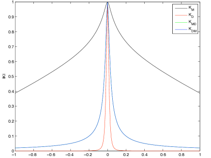
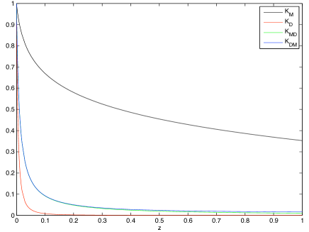
Figure 2. (Left) 3d transverse profiles with FWHM $=1.37(K_{\rm M}),0.03(K_{\rm D}),0.07(K_{\rm MD},K_{\rm DM})$; (Right) 3d longitudinal profiles with FWHM $=0.3565(K_{\rm M}),0.00421(K_{\rm D}),0.00947(K_{\rm DM},K_{\rm MD}).$ Note that the transverse profiles of the $K_{\rm MD}$ and $K_{\rm DM}$ coincide.

For $\mathbf{r}^{\prime}=\mathbf{r}_{0}^{\prime}$ and $\mathbf{r}=\mathbf{r}_{0}$, $\mathbf{r}-\mathbf{r}^{\prime}$ is orthogonal to $A$ and thus $|\nabla G|\sim|\partial G/\partial n|$. Therefore the leading order transverse profile for $K_{\rm D}(\mathbf{r},\mathbf{r}_{0})$ is given approximately by

(33) $${1\over k}\int{\delta\over(x^{\prime 2}+y^{\prime 2}+\delta^{2})^{3/2}}\times{\delta\over((x-x^{\prime})^{2}+y^{\prime 2}+\delta^{2})^{3/2}}dx^{\prime}dy^{\prime}.$$

The integrand in (33) has a different singularity than that in (29). Indeed, for $x=\delta^{\alpha}$, the dominant contribution to (33) comes from the disks of radius $\delta$ around $(0,0)$ and $(\delta^{\alpha},0)$ which is easily estimated to be

$$K_{\rm D}(\mathbf{r},\mathbf{r}_{0})\sim\delta^{1-3\alpha},\quad\alpha\in[0,1].$$

By contrast, $K_{\rm D}(\mathbf{r}_{0},\mathbf{r}_{0})\sim\delta^{-2}$. Hence the focal spot size in this case is smaller than $\delta^{\alpha},\forall\alpha\in[0,1)$ asymptotically. We conclude that the focal spot size for the dipole TR is essentially $O(\delta)$ and that the dipole TR can in principle break the diffraction limit to achieve an arbitrarily fine resolution by bring the TRM sufficiently close to the source.

4.3. Transverse resolution of mixed mode TR

By the same analysis as before, the integrals (12) and (13) can be approximated by, respectively,

(34) $$\int{1\over(x^{\prime 2}+y^{\prime 2}+\delta^{2})^{1/2}}\times{\delta\over((x-x^{\prime})^{2}+y^{\prime 2}+\delta^{2})^{3/2}}dx^{\prime}dy^{\prime}$$

(35) $$-\int{\delta\over(x^{\prime 2}+y^{\prime 2}+\delta^{2})^{3/2}}\times{1\over((x-x^{\prime})^{2}+y^{\prime 2}+\delta^{2})^{1/2}}dx^{\prime}dy^{\prime}.$$

Set $x=\delta^{\alpha},0\leq\alpha<1$. In the case of (34), the dominant contribution ($\sim\delta^{-\alpha}$) comes from integration around $(\delta^{\alpha},0)$ for $\alpha<1$ while, in the case of (35), the dominant contribution ($\sim\delta^{-\alpha}$) comes from integration around $(0,0)$. In both cases $K_{\rm MD}(\mathbf{r}_{0},\mathbf{r}_{0})\sim K_{\rm DM}(\mathbf{r}_{0},\mathbf{r}_{0})\sim\delta^{-1}$. Hence the focal spot size is smaller than $\delta^{\alpha},\forall\alpha\in[0,1)$ asymptotically.

We conclude that the focal spot size for the mixed mode TR is essentially $O(\delta)$ and that the mixed mode TR can achieve an arbitrarily fine resolution as the TRM approaches the point source. Moreover, the fact that the maximum values of the point-spread functions are inversely proportional to the focal spot size is consistent with the cut-off version of (23) in the following sense. Truncate the Green function (26) at the level $\delta^{-1}$ as in (25). Then the asymptotic spot size of the resulting function is $O(\delta)$. In other words, the mixed mode TR of near field recovers qualitatively the asymptotic behavior of the Green function near the source point.

When the superresolution terms from $K_{\rm DM}$ and $K_{\rm MD}$ combine in $K_{\rm PB}$, they cancel each other resulting in diffraction-limited focal spot.

In Figure 2 the normalized transverse and longitudinal profiles are shown and their resolutions calculated for various TR schemes. The profiles are normalized to be unity at the source location. In the simulation, we use $\lambda=2\pi$, $A=2\lambda$ and $\mathbf{r}_{0}=(0.01,0,0)$. Before normalization, the $K_{\rm M}$ curve has the maximum less than $0.5$ and hence is far from the square-root asymptotic regime discussed in the paragraph following (32).

4.4. Two-dimensional case

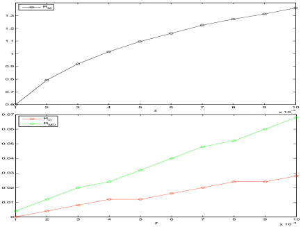
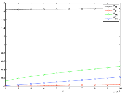
Figure 3. The transverse resolution of various TR schemes in three (left) and two (right) dimensions. The linear behavior of $R^{2}_{\rm MD}$ in the right plot demonstrates the square-root behavior of $R_{\rm MD}$ in two dimensions.

It is instructive to compare the scaling behavior of resolution in two and three dimensions. In two dimensions, (33) becomes

(36) $${1\over k}\int{\delta\over x^{\prime 2}+\delta^{2}}\times{\delta\over(x-x^{\prime})^{2}+\delta^{2}}dx^{\prime}.$$

The same calculation shows that

$$K_{\rm D}(\mathbf{r},\mathbf{r}_{0})\sim\delta^{1-2\alpha},\quad\alpha\in[0,1]$$

and $K_{\rm D}(\mathbf{r}_{0},\mathbf{r}_{0})\sim\delta^{-1}$. The $K_{\rm D}$-resolution asymptotic is given by $\delta^{\alpha},\alpha=1$.

For the mixed mode, (34) and (35) become

(38) $${1\over k}\int\log{(x^{\prime 2}+\delta^{2})^{-1/2}}\times{\delta\over(x-x^{\prime})^{2}+\delta^{2}}dx^{\prime}$$

$$-{1\over k}\int{\delta\over x^{\prime 2}+\delta^{2}}\times\log{((x-x^{\prime})^{2}+\delta^{2})^{-1/2}}dx^{\prime}$$

yielding

$$K_{\rm MD}(\mathbf{r},\mathbf{r}_{0}),K_{\rm DM}(\mathbf{r},\mathbf{r}_{0})\sim\alpha\left(-\log{\delta}\right)^{2},\quad\alpha\in[0,1]$$

and $K_{\rm MD}(\mathbf{r}_{0},\mathbf{r}_{0}),K_{\rm DM}(\mathbf{r}_{0},\mathbf{r}_{0})\sim\left(-\log{\delta}\right)^{2}$. Hence, the asymptotic resolution for the mixed mode TR is given by $\delta^{\alpha},\alpha=1/2$. Empirically, the square-root regime for the mixed mode TR in two dimensions sets in much earlier than the monopole TR in three dimensions. Here lies the main difference between the two and three dimensional cases. Namely, in two dimensions the transverse resolution for the mixed mode TR is proportional to the square-root of the distance between the source and TRM.

For the monopole TR in two dimensions, $K_{\rm M}$ is uniformly bounded w.r.t. $\delta$ and the resolution can not be deduced from the asymptotic analysis. It is likely though that the monopole TR resolution is qualitatively independent of $\delta$. This is amply confirmed by our numerical simulations (Figure 3).

In Figure 3 the transverse resolutions, denoted by $R_{\rm X},{\rm X=M,D,MD,DM}$, for the respective TR schemes as a function of the distance between the source and TRM are plotted for the range $[0.001,0.01]$. The dipole resolution $R_{\rm D}$ exhibits the linear behavior in two and three dimensions and the mixed mode resolution $R_{\rm MD},R_{\rm DM}$ exhibits the linear behavior in three dimensions and square-root behavior in two dimensions. Both the dipole and mixed mode resolutions are order of magnitude better than the monopole resolution.

In Figure 4 the normalized transverse and longitudinal profiles in two dimensions are shown and FWHM calculated for various TR schemes with the same physical parameters as in Figure 2. The unnormalized transverse profile for the mixed mode TR has the maximum about 6. The dipole resolution is much better than the mixed mode resolution which in turn is much better than the monopole resolution in both the transverse and longitudinal directions.

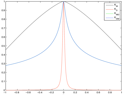
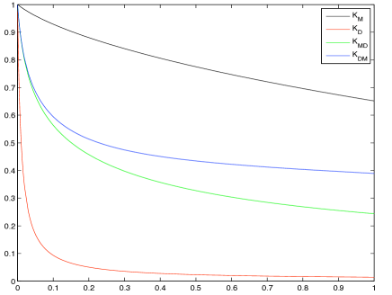
Figure 4. (Left) 2d transverse profiles with FWHM$=1.87(K_{\rm M}),0.05(K_{\rm D}),0.47(K_{\rm DM},K_{\rm MD})$; (Right) 2d longitudinal profiles: FWHM$=1(K_{\rm M}),0.009(K_{\rm D}),0.148(K_{\rm MD}),0.22(K_{\rm DM}).$ Note that the transverse profiles for the $K_{\rm MD}$ and $K_{\rm DM}$ coincide.

In summary, in the case of a monopole source the dipole TR produces the best resolution in both transverse and longitudinal directions, roughly in proportion to the distance between the source and TRM. The mixed mode TR can deliver nearly the same performance in three dimensions and roughly the square-root resolution in the transverse direction in two dimensions. Between the two mixed mode TR schemes, $K_{\rm MD}$ is still better than $K_{\rm DM}$ in the longitudinal direction. A simple explanation for the superior resolution of TRM involving the dipole field is that a dipole source has a stronger singularity than a monopole source (cf. (27) versus (26))

5. Approximate TR is biased

We have already seen that the perfect TR described by (7) with $G=G_{0}$ is diffraction-limited and contains no evanescent component of the initial outgoing field (see the remark following (24)).

For the half space (domain (iii) of Figure 1), the result is similar: Suppose the initial wave field is perfectly phase-conjugated on the TRM (i.e. the boundary condition (21) is satisfied exactly by, say, the scheme $K_{\rm MD}$). Then in the interior of the half space the homogenous components of the initial wave are perfectly phase-conjugated but the evanescent components are exponentially damped by the factor

$$e^{-2kz\sqrt{s_{1}^{2}+s_{2}^{2}-1}},\quad s_{1}^{2}+s_{2}^{2}>1$$

depending on the distance $z$ from the TRM to the field point $(z,\mathbf{x})$ (Appendix C).

On the other hand, for the paraxial wave (45), perfect phase conjugation on one plane implies perfect phase conjugation in the half space due to the fact that the paraxial wave field is uniquely determined by the direction of propagation and the initial condition on one plane (Appendix C). As a consequence, $v_{\rm M}$ and $K_{\rm M}$ are perfect TR schemes in their respective contexts. In particular, $K_{\rm M}$ can focus perfectly back on the location of the point source in the paraxial approximation.

The perfect focusing of time reversed paraxial wave is, of course, unphysical because the evanescent waves are not accounted for. The other aspect that is more impractical than unphysical with the perfect conjugation of the homogeneous component of the spherical wave, is that an infinite aperture ($A=\mathbb{R}^{2}$) is required for such a result.

In this section, we show that when $D$ is a half space and $A$ is bounded, the maximum point of the TR focal spot does not correspond to the exact source location $\mathbf{r}_{0}$ in general. In contrast, when $A=\mathbb{R}^{2}$ in the paraxial regime, since $K_{\rm M}$ is a perfect TR scheme for the paraxial wave, the focal spot is always centered.

This bias effect tends to be much more pronounced in the longitudinal direction. As the aperture of TRM increases, the transverse offset (bias) decreases while the longitudinal offset may persist if there is insufficient scattering in the medium, cf. Section 6. This is why we consider only the transverse resolution in the previous section.

Let us recast the problem in more general terms. Let $\phi(\mathbf{r},\mathbf{r}^{\prime})$ be the phase of $G(\mathbf{r},\mathbf{r}^{\prime})$ and define

(39) $$P_{\rm M}(\mathbf{r}) = \left|\int_{A}G^{*}(\mathbf{r}^{\prime},\mathbf{r}_{0})e^{i\phi(\mathbf{r},\mathbf{r}^{\prime})}W(\mathbf{r},\mathbf{r}^{\prime})d\sigma(\mathbf{r}^{\prime})\right|^{2}$$

where $W(\mathbf{r},\mathbf{r}^{\prime})$ is a non-negative function. The monopole TR kernel $K_{\rm M}$ corresponds to $W(\mathbf{r},\mathbf{r}^{\prime})=|G(\mathbf{r},\mathbf{r}^{\prime})|$.

Direct calculation of $\nabla P_{\rm M}(\mathbf{r}_{0})$ yields

$$\nabla P_{\rm M}(\mathbf{r}_{0})$$

$$= \int_{A\times A}|G^{*}(\mathbf{r}^{\prime},\mathbf{r}_{0})||G(\mathbf{r}^{\prime\prime},\mathbf{r}_{0})|W(\mathbf{r}_{0},\mathbf{r}^{\prime})W(\mathbf{r}_{0},\mathbf{r}^{\prime\prime})(i\nabla\phi(\mathbf{r}_{0},\mathbf{r}^{\prime})-i\nabla\phi(\mathbf{r}_{0},\mathbf{r}^{\prime\prime}))d\sigma(\mathbf{r}^{\prime})d\sigma(\mathbf{r}^{\prime\prime})$$

$$+\int_{A\times A}|G^{*}(\mathbf{r}^{\prime},\mathbf{r}_{0})||G(\mathbf{r}^{\prime\prime},\mathbf{r}_{0})|\nabla\left(W(\mathbf{r},\mathbf{r}^{\prime})W(\mathbf{r},\mathbf{r}^{\prime\prime})\right)_{\mathbf{r}=\mathbf{r}_{0}}d\sigma(\mathbf{r}^{\prime})d\sigma(\mathbf{r}^{\prime\prime}).$$

The first term vanishes due to anti-symmetry with respect to $\mathbf{r}^{\prime},\mathbf{r}^{\prime\prime}$.

Consider the case of a planar TRM on the plane $z=0$ with the paraxial wave propagating in the $z$-direction (Appendix A). Suppose the medium inhomogeneities act like a phase object affecting only the phase of the free propagator. Namely, $G(z,\mathbf{x},z^{\prime},\mathbf{x}^{\prime})$ takes the form

(40) $$G(z,\mathbf{x},z^{\prime},\mathbf{x}^{\prime})=-{1\over 4\pi(z-z^{\prime})}e^{ik(z-z^{\prime})}e^{i{k|\mathbf{x}-\mathbf{x}^{\prime}|^{2}\over 2(z-z^{\prime})}}e^{i\theta(z,\mathbf{x},z^{\prime},\mathbf{x}^{\prime})},\quad\mathbf{x},\mathbf{x}^{\prime}\in\mathbb{R}^{2}.$$

Note that for (40) the expression (39) is divergent and thus invalid at $\mathbf{r}=\mathbf{r}_{0}$ if $A=\mathbb{R}^{2}$.

For a finite aperture, $W(\mathbf{r},\mathbf{r}^{\prime})=(4\pi|z-z^{\prime}|)^{-1}$ and thus $\nabla\left(W(\mathbf{r},\mathbf{r}^{\prime})W(\mathbf{r},\mathbf{r}^{\prime\prime})\right)_{\mathbf{r}=\mathbf{r}_{0}}$ points in the negative $z$ direction and consequently $\mathbf{r}_{0}$ tends to be farther away from $A$ than the maximum point of $P_{\rm M}$. In other words, the focal spot of the monopole TR tends to be closer to $A$ than the source location. Even in the case of a closed cavity the offset (bias) is reduced but not completely eliminated except for special cases.

Now let us change the perspective and think of TR as a means of imaging a point source in a perfectly known medium. In this context a few widely used $W(\mathbf{r},\mathbf{r}^{\prime})$’s are:

$$W(\mathbf{r},\mathbf{r}^{\prime}) = |G(\mathbf{r},\mathbf{r}^{\prime})|^{-1}\quad\mbox{(the inverse filter)},$$

$$W(\mathbf{r},\mathbf{r}^{\prime}) = W(\mathbf{r}^{\prime})/\sqrt{\int_{A}|W(\mathbf{r}^{\prime\prime})|^{2}d\sigma(\mathbf{r}^{\prime\prime})},\,\,\forall W\in L^{2}(A,d\sigma)\quad\mbox{(the phase processor)},$$

$$W(\mathbf{r},\mathbf{r}^{\prime}) = |G(\mathbf{r},\mathbf{r}^{\prime})|/\sqrt{\int_{A}|G(\mathbf{r},\mathbf{r}^{\prime\prime})|^{2}d\sigma(\mathbf{r}^{\prime\prime})}\quad\mbox{ (the conventional matched field processor)}.$$

For the inverse filter, $\nabla(W(\mathbf{r},\mathbf{r}^{\prime})W(\mathbf{r},\mathbf{r}^{\prime\prime}))_{\mathbf{r}=\mathbf{r}_{0}}$ and thus $\nabla P_{\rm M}(\mathbf{r}_{0})$ tend to point away from the TR mirror $A$ and hence the source location tends to be closer to $A$ than the maximum point of $P_{\rm M}$. Again, when $A=\partial D$ or in the far field regime this offset can be reduced.

Direct substitution shows that $\nabla P_{\rm M}(\mathbf{r}_{0})=0$ for the two latter choices of $W$. Moreover, $\mathbf{r}_{0}$ is the maximum point of $P_{\rm M}$ for both choices of $W$. In the case of the $W$-weighted phase processor, we clearly have

$$P_{\rm M}(\mathbf{r})\leq\int_{A}|G^{*}(\mathbf{r}^{\prime},\mathbf{r}_{0})|W(\mathbf{r}^{\prime})d\sigma(\mathbf{r}^{\prime})=P_{\rm M}(\mathbf{r}_{0}).$$

In the case of the conventional matched field processing, it is well known [2, 25] that

(41) $$V(\mathbf{r}_{0},\mathbf{r}^{\prime})=G(\mathbf{r}_{0},\mathbf{r}^{\prime})/\sqrt{\int_{A}|G(\mathbf{r}_{0},\mathbf{r}^{\prime})|^{2}d\sigma(\mathbf{r}^{\prime})}$$

is the solution to the optimization problem: Maximize the quantity

$$\left|\int_{A}G^{*}(\mathbf{r}^{\prime},\mathbf{r}_{0})V(\mathbf{r}^{\prime})d\sigma(\mathbf{r}^{\prime})\right|^{2}$$

over $V$ subject to the constraint

(42) $$\int|V|^{2}(\mathbf{r}^{\prime})d\sigma(\mathbf{r}^{\prime})=1.$$

Therefore

$$P_{\rm M}(\mathbf{r})=\int_{A}G^{*}(\mathbf{r}^{\prime},\mathbf{r}_{0})V(\mathbf{r},\mathbf{r}^{\prime})d\sigma(\mathbf{r}^{\prime})$$

is maximized at $\mathbf{r}=\mathbf{r}_{0}$ with the conventional matched field processing.

In summary, as an imaging method both TR and the inverse filter are generally biased; the former tends to underestimate the range of the source while the latter tends to overestimate it. The conventional matched field processor is unbiased and produces the optimal signal-to-noise ratio. The phase processor, which uses only the phase of the Green function, is a simple alternative to the conventional matched field processor.

Moreover, in the regime described by (40), $|G(\mathbf{r},\mathbf{r}^{\prime})|$ is a function of the distance between the source point and the TRM. In such a case the conventional matched field processor coincides with the phase processor with $W(\mathbf{r}^{\prime})=\mathbb{I}_{A}/|A|^{1/2}$ independent of $\mathbf{r}^{\prime}$.

Similar conclusions can be drawn for the pure dipole case with

(43) $$P_{\rm D}(\mathbf{r}) = \left|\int_{A}{\partial G^{*}(\mathbf{r}^{\prime},\mathbf{r}_{0})\over\partial n}e^{i\psi(\mathbf{r},\mathbf{r}^{\prime})}W(\mathbf{r},\mathbf{r}^{\prime})d\sigma(\mathbf{r}^{\prime})\right|^{2}$$

where $\psi(\mathbf{r},\mathbf{r}^{\prime})$ is the phase of $\partial G(\mathbf{r},\mathbf{r}^{\prime})/\partial n$. $P_{\rm D}$ can be analyzed as above with $G$ replaced by its normal derivative.

For $K_{\rm MD},K_{\rm DM}$, consider the paraxial regime for which (3.1) is valid. Each term on the right hand side of (3.1) can be analyzed as before. The result is that the mixed mode TR’s are biased, especially in the longitudinal direction, just like the monopole and dipole TR’s.

6. Randomness eliminates bias

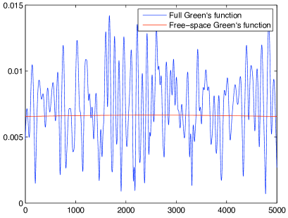
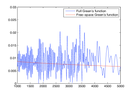
Figure 5. The transverse (left), at $x=5000$, and longitudinal (right), at $y=2500$, profiles of the intensity of the $2-d$ Green function at wavelength $70$ with 1000 particles randomly distributed in $[2000,4000]\times[0,5000]$ and source (not shown) at $(-5000,2500)$ whose $n^{2}-1$ is $70$. (Reproduced from [16])

In this section, we explain how randomness can make the TR focal spot centered at the location of the source point.

Consider typical profiles of the Green function in a multiple scattering medium as depicted in Figure 5. A main feature of the intensity profiles is the rapid fluctuations in the transverse and longitudinal directions. These fluctuations upon differentiation and averaging (integration over $A\times A$) as in the expression

(44) $${\nabla P_{\rm M}(\mathbf{r}_{0})}={1\over 2}\int_{A\times A}\nabla\left|G(\mathbf{r},\mathbf{r}^{\prime})G(\mathbf{r},\mathbf{r}^{\prime\prime})\right|^{2}_{\mathbf{r}=\mathbf{r}_{0}}d\sigma(\mathbf{r}^{\prime})d\sigma(\mathbf{r}^{\prime\prime})$$

essentially cancel one another.

More precisely, the degrees of scattering and randomness can be measured by the spatial spread of the propagation channel. If the spatial spread increases to infinity, then the TRM acquires an effective aperture that is proportional to the spatial spread [4, 15]. Then, as per discussion at the beginning of Section 5, the accuracy of approximate TR’s improve and the focal spot becomes more centered and sharper.

Moreover, counterintuitively, the TR image can avoid statistical fluctuations if the medium is sufficiently random. Let us recall some analytical results from the literature.

Consider TR in a random medium occupying a half space with TRM on the planar boundary. When the random channel is the Rayleigh fading regime (i.e. obeying zero-mean Gaussian statistics) with a divergent spatial spread the monopole TR (10) with TRM’s aperture much larger than the coherence length $\ell_{c}$ will focus on the source point with a spot size $\sim\ell_{c}$ [13, 14]. The conventional coherence theory suggests that the coherence length is of the order of wavelength [23]. However, spatial correlations of much smaller extent has been recently measured in the near field of random media [1]. This effect in conjunction with the preceding theory may be the key to understanding the subwavelength focusing observed in the time reversal experiment reported in [21].

The result of stability and focusing is a special case of what was originally established for the setting of multiple frequencies and multiple source points [13, 14]. With straightforward modification of the arguments in [13, 14] the same result can be extended to any TR of the types (10)-(13) in the paraxial regime, the only difference being in the asymptotic shape of the focal spot. Experiments show consistently similar results on stability and focusing properties [17, 21, 27].

In conclusion, random fluctuations in the intensity of Green’s function is a necessary condition for the desired focusing property of time reversal with a finite aperture.

7. Conclusion

We have reexamined various time reversal schemes that can be employed from the boundary of a domain; they involve monopole and/or dipole fields.

We have explored their relationships in the paraxial regime. For the boundary behavior, we show that for paraxial wave only the monopole TR scheme satisfies the exact boundary condition while for the spherical wave only the MD-mode TR scheme satisfies the exact boundary condition. We have also shown that for the paraxial wave the standard monopole TRM produces the perfect result in the entire domain but for the near field the monopole TRM can hardly achieve subwavelength focusing. On the other hand, the dipole TRM is approximate in the paraxial regime but is capable of producing a focal spot size linearly proportional to the distance from TRM to the source location, thus focusing on a subwavelength scale when the TRM is sufficiently close to the source point. The mixed mode TRM has the similar (linear) behavior in three dimensions but the square-root asymptotic in two dimensions. The monopole TRM is, if possible at all, ineffective to focus below wavelength.

We have seen how two mixed mode effects combine in the so called perfect TR scheme for a closed cavity and cancel their respective subwavelength focusing property. The perfect TRM is “perfect” only for a source-free initial field.

We have examined an often neglected effect of biased focusing associated with TRM of a finite aperture in a weak- or non-scattering medium. This effect pertains to all five TR schemes discussed in the paper. In a multiply scattering medium, the bias is greatly reduced and the focal spot becomes centered at the source location. The removal of bias by random scattering is attributed to the enlarged effective aperture and the random fluctuations in the intensity of the Green function.

Appendix A Mixed mode TR for paraxial wave

Let $z\in\mathbb{R}$ be the longitudinal coordinate and $\mathbf{x}\in\mathbb{R}^{2}$ the transverse coordinates. Let $G^{\pm}_{\rm P}(z,\mathbf{x},z^{\prime},\mathbf{x}^{\prime})$ be the Green functions for the paraxial wave equation

(45) $$\pm i\frac{\partial}{\partial z}\Psi+\frac{1}{2k}\Delta_{\rm T}\Psi+{k\over 2}(n^{2}(z,\mathbf{x})-1)\Psi=0$$

where $\Delta_{\rm T}$ is the transverse Laplacian. The plus sign represents positive $z$ propagating wave and minus sign negative $z$ propagating wave.

The full Green function $G(z,\mathbf{x},z^{\prime},\mathbf{x}^{\prime})$ in the paraxial regime can be expressed as

(46) $$G(z,\mathbf{x},z^{\prime},\mathbf{x}^{\prime}) = {ie^{ik(z-z^{\prime})}\over 2k}G^{-}_{\rm P}(z,\mathbf{x},z^{\prime},\mathbf{x}^{\prime}),\quad z>z^{\prime}$$

(47) $$G(z,\mathbf{x},z^{\prime},\mathbf{x}^{\prime}) = {ie^{ik(z^{\prime}-z)}\over 2k}G^{-}_{\rm P}(z,\mathbf{x},z^{\prime},\mathbf{x}^{\prime}),\quad z<z^{\prime}$$

Let $D=\{z>0\}$, the plane $z=0$ be occupied by the TRM and $\mathbf{r}_{0}=(z_{0},\mathbf{x}_{0})$ be the location of the source. Assume that the TRM is away from the medium inhomogeneities i.e. $n(0,\mathbf{x})=1$. Then $K_{\rm MD}$ can be written as

$$K_{\rm MD}(\mathbf{r},\mathbf{r}_{0}) = -{ie^{ik(z-z_{0})}\over 4k}\int G_{\rm P}^{-*}(0,\mathbf{x}^{\prime},z_{0},\mathbf{x}_{0})G^{-}_{\rm P}(0,\mathbf{x}^{\prime},z,\mathbf{x})d\mathbf{x}^{\prime}$$

$$+{e^{ik(z-z_{0})}\over 4k^{2}}\int G_{\rm P}^{-*}(0,\mathbf{x}^{\prime},z_{0},\mathbf{x}_{0}){\partial\over\partial z^{\prime}}G^{-}_{\rm P}(z^{\prime},\mathbf{x}^{\prime},z,\mathbf{x})|_{z^{\prime}=0}d\mathbf{x}^{\prime}.$$

By the assumption $n(0,\mathbf{x})=1$ and (45), we have

$$K_{\rm MD}(\mathbf{r},\mathbf{r}_{0}) = -{ie^{ik(z-z_{0})}\over 4k}\int G_{\rm P}^{-*}(0,\mathbf{x}^{\prime},z_{0},\mathbf{x}_{0})G^{-}_{\rm P}(0,\mathbf{x}^{\prime},z,\mathbf{x})d\mathbf{x}^{\prime}$$

$$+{ie^{ik(z-z_{0})}\over 8k^{3}}\int G_{\rm P}^{-*}(0,\mathbf{x}^{\prime},z_{0},\mathbf{x}_{0})\Delta^{\prime}_{\rm T}G^{-}_{\rm P}(0,\mathbf{x}^{\prime},z,\mathbf{x})d\mathbf{x}^{\prime}$$

$$= -ik\int G^{*}(0,\mathbf{x}^{\prime},z_{0},\mathbf{x}_{0})G(0,\mathbf{x}^{\prime},z,\mathbf{x})d\mathbf{x}^{\prime}$$

$$+{i\over 2k}\int\nabla^{\prime}_{\rm T}G^{*}(0,\mathbf{x}^{\prime},z_{0},\mathbf{x}_{0})\cdot\nabla^{\prime}_{\rm T}G(0,\mathbf{x}^{\prime},z,\mathbf{x})d\mathbf{x}^{\prime}$$

after integration by parts. The result for $K_{\rm DM}$ can be likewise derived.

Appendix B Boundary values

B.1. Paraxial wave

Let us first focus on the boundary values of (14)-(17). Let $u(z,\mathbf{x})$ be a paraxial wave propagating in the negative $z$ direction which can be written as

$$e^{-ikz}\Psi(z,\mathbf{x})$$

where $\Psi$ is the solution of eq. (45) with the minus sign.

In the paraxial regime with $n(0,\mathbf{x})=1$, we have from (46) and (45) that

$$v_{\rm M}(0,\mathbf{x}) = \int u^{*}(0,\mathbf{x}^{\prime})G^{+}_{\rm P}(0,\mathbf{x},0,\mathbf{x}^{\prime})d\mathbf{x}^{\prime}$$

$$v_{\rm D}(0,\mathbf{x}) = -{i\over k}\int\Delta_{\rm T}u^{*}(0,\mathbf{x}^{\prime})G^{+}_{\rm P}(0,\mathbf{x},0,\mathbf{x}^{\prime})d\mathbf{x}^{\prime}-{i\over 2k^{3}}\int\Delta_{\rm T}^{2}u^{*}(0,\mathbf{x}^{\prime})G^{+}_{\rm P}(0,\mathbf{x},0,\mathbf{x}^{\prime})d\mathbf{x}^{\prime}$$

$$v_{\rm MD}(0,\mathbf{x}) = {1\over 2}\int u^{*}(0,\mathbf{x}^{\prime})G^{+}_{\rm P}(0,\mathbf{x},0,\mathbf{x}^{\prime})d\mathbf{x}^{\prime}+{1\over 4k^{2}}\int\Delta_{\rm T}u^{*}(0,\mathbf{x}^{\prime})G^{+}_{\rm P}(0,\mathbf{x},0,\mathbf{x}^{\prime})d\mathbf{x}^{\prime}$$

$$v_{\rm DM}(0,\mathbf{x}) = {1\over 2}\int u^{*}(0,\mathbf{x}^{\prime})G^{+}_{\rm P}(0,\mathbf{x},0,\mathbf{x}^{\prime})d\mathbf{x}^{\prime}+{1\over 4k^{2}}\int\Delta_{\rm T}u^{*}(0,\mathbf{x}^{\prime})G^{+}_{\rm P}(0,\mathbf{x},0,\mathbf{x}^{\prime})d\mathbf{x}^{\prime}$$

where $u$ is a paraxial wave propagating in the negative $z$ direction. Setting $G^{\pm}_{\rm P}(0,\mathbf{x},0,\mathbf{x}^{\prime})=\delta(\mathbf{x}-\mathbf{x}^{\prime})$, we obtain the following boundary conditions

$$v_{\rm M}(0,\mathbf{x}) = u^{*}(0,\mathbf{x})$$

$$v_{\rm D}(0,\mathbf{x}) = -{i\over k}\Delta_{\rm T}u^{*}(0,\mathbf{x}^{\prime})-{i\over 2k^{3}}\Delta_{\rm T}^{2}u^{*}(0,\mathbf{x}^{\prime})$$

$$v_{\rm MD}(0,\mathbf{x}) = {1\over 2}u^{*}(0,\mathbf{x})+{1\over 4k^{2}}\Delta_{\rm T}u^{*}(0,\mathbf{x})$$

$$v_{\rm DM}(0,\mathbf{x}) = {1\over 2}u^{*}(0,\mathbf{x})+{1\over 4k^{2}}\Delta_{\rm T}u^{*}(0,\mathbf{x})$$

$$v_{\rm PB}(0,\mathbf{x}) = u^{*}(0,\mathbf{x})+{1\over 2k^{2}}\Delta_{\rm T}u^{*}(0,\mathbf{x}).$$

The kernel $K_{\rm X},{\rm X}={\rm M,D,MD,DM,PB}$ satisfy the similar boundary properties. In other words, only the monopole TR gives the correct boundary values in the case of paraxial wave propagating in the half space.

B.2. Spherical wave

Consider the half space $D=\{z>0\}$ with $A=\{z=0\}$. Assume $G=G_{0}$, the free space Green function.

Differentiating the Weyl representation for $G_{0}$ with respect to $z^{\prime}$, we find that

(50) $${\partial\over\partial z^{\prime}}G_{0}(z,\mathbf{x},z^{\prime},\mathbf{x}^{\prime})\left.\right|_{z=z^{\prime}=0}={1\over 2}\delta(\mathbf{x}-\mathbf{x}^{\prime}).$$

From (50) it is immediately clear that

$$v_{\rm MD}(0,\mathbf{x})={1\over 2}u^{*}(0,\mathbf{x}),\quad K_{\rm MD}(0,\mathbf{x})={1\over 2}G^{*}(0,\mathbf{x},z_{0},\mathbf{x}_{0}).$$

However, neither $v_{\rm DM}$ nor $K_{\rm DM}$ satisfies the boundary condition as we show now.

In the neighborhood of $A$, the wave field $u$ in $D$ can be represented in terms of the plane wave spectrum:

(51) $$u(x,y,z) = \int{ds_{1}ds_{2}}e^{ik(s_{1}x+s_{2}y)}e^{iks_{3}z}A(s_{1},s_{2})+\int{ds_{1}ds_{2}}e^{ik(s_{1}x+s_{2}y)}e^{-iks_{3}z}B(s_{1},s_{2})$$

where $s_{3}$ is given in (24). Consider for simplicity one-way wave with, say, $B\equiv 0$. Then the phase-conjugated field has the form

$$u^{*}(x,y,z) = \int_{s_{1}^{2}+s_{2}^{2}\leq 1}{ds_{1}ds_{2}}e^{ik(s_{1}x+s_{2}y)}e^{-iks_{3}z}A^{*}(-s_{1},-s_{2})$$

$$+\int_{s_{1}^{2}+s_{2}^{2}>1}{ds_{1}ds_{2}}e^{ik(s_{1}x+s_{2}y)}e^{iks_{3}z}A^{*}(-s_{1},-s_{2})$$

and thus

$${\partial\over\partial z}u^{*}(x,y,0) = ik\int{ds_{1}ds_{2}}e^{ik(s_{1}x+s_{2}y)}s_{3}A^{*}(-s_{1},-s_{2})\left[-I_{\{s_{1}^{2}+s_{2}^{2}\leq 1\}}+I_{\{s_{1}^{2}+s_{2}^{2}>1\}}\right].$$

where $I_{S}$ is the indicator function of the set $S$. By Plancherel’s identity we obtain

$$v_{\rm DM}(0,\mathbf{x}) = 2\pi\int{ds_{1}ds_{2}}e^{ik(s_{1}x+s_{2}y)}A^{*}(-s_{1},-s_{2})\left[-I_{\{s_{1}^{2}+s_{2}^{2}\leq 1\}}+I_{\{s_{1}^{2}+s_{2}^{2}>1\}}\right]$$

$$\neq 2\pi u^{*}(0,\mathbf{x}).$$

Namely, no constant multiple of $v_{\rm DM}$ satisfies the boundary condition.

Likewise, one can show that none of the other TR schemes than $v_{\rm MD},K_{\rm MD}$ satisfies the boundary condition, with some adjustable constant factor.

Appendix C One-plane TRM in a half space

Consider the half space $D=\{z>0\}$ with $A=\{z=0\}$ and point source located at $(z_{0},\mathbf{x}_{0}),z_{0}>0$, Figure 6. We assume that the medium inhomogeneities $n^{2}-1$ is away from the TRM so that the gap $D^{-}$ is a non-empty infinite slab. Figure 6.

First we observe that for the paraxial wave, perfect phase conjugation on $z=0$ implies perfect phase conjugation throughout the domain $D$. This can be shown as follows.

Let $u(z,\mathbf{x})=e^{-ikz}\Psi^{-}(z,\mathbf{x})$ be the initial wave propagating in the negative $z$ direction where $\Psi^{-}$ satisfies (45) with the minus sign. If $u(0,\mathbf{x})$ is perfectly conjugated by, say, either the scheme described by $v_{\rm M}$ or $v_{\rm PB}$, then the resulting field, denoted by $v(z,\mathbf{x})$, is given by

$$v(z,\mathbf{x})=e^{ikz}\Psi^{+}(z,\mathbf{x})$$

where $\Psi^{+}$ satisfies (45) with the plus sign and the initial condition

$$\Psi^{+}(0,\mathbf{x})=\Psi^{-*}(0,\mathbf{x}).$$

Now since $\Psi^{-*}(z,\mathbf{x})$ satisfies (45) with the plus sign and the initial condition $\Psi^{+}(0,\mathbf{x})$, we have from the uniqueness theorem for the initial value problem of (45) that

$$\Psi^{+}(z,\mathbf{x})=\Psi^{-*}(z,\mathbf{x})$$

and consequently

$$v(z,\mathbf{x})=u^{*}(z,\mathbf{x}),\quad z>0.$$

The same argument and conclusion apply to the paraxial wave with a point source.

The case with the spherical wave is similar but more subtle since the evanescent wave is involved. It can be shown that the Green function in $D^{-}\cap\{z<z_{0}\}$ can be expressed as superposition of plane waves propagating in the negative $z$ direction

(52) $$G(\mathbf{r},\mathbf{r}_{0})=\int{ds_{1}ds_{2}}e^{ik(s_{1}x+s_{2}y)}e^{-iks_{3}z}B(s_{1},s_{2}),\quad\mathbf{r}\in D^{-}\cap\{z<z_{0}\}$$

in analogy to (51).

Figure 6. The dark area represents the scattering domain $S$. The asterisk, $*$, represents the source point $\mathbf{r}_{0}$ which may be anywhere in $D$.

Let $W$ be a source-free field propagating across $z=0$ into $D$ and be represented as

(53) $$W(\mathbf{r})=\int{ds_{1}ds_{2}}e^{ik(s_{1}x+s_{2}y)}e^{iks_{3}z}A(s_{1},s_{2}),\quad\mathbf{r}\in D^{-}.$$

Note the sign in the exponent associated with $z$ here is different from that in (52) since they propagate in the opposite directions. Suppose $W$ is the phase conjugate field of $G$ at $z=0$, i.e. $W^{*}(x,y,0)=G(x,y,0,\mathbf{r}_{0}),\forall x,y.$ For $z=0$, equating (53) with (52) conjugated we obtain the condition

(54) $$A(s_{1},s_{2}) = B^{*}(-s_{1},-s_{2}).$$

This result is first observed in [22].

Let $W_{H}$ and $W_{E}$ be, respectively, the homogeneous and the evanescent components of $W$, corresponding to, respectively, the integration (53) restricted to $s_{1}^{2}+s_{2}^{2}\leq 1$ and $s_{1}^{2}+s_{2}^{2}>1$. The homogeneous and the evanescent components $G_{H},G_{I}$ of (52) are defined analogously. Then (54) lead to, respectively,

(55) $$W_{H}^{*}(\mathbf{r}) = G_{H}(\mathbf{r}),\quad\mathbf{r}\in D^{-}$$

(56) $$W_{I}^{*}(\mathbf{r}) = \int{ds_{1}ds_{2}}e^{ik(s_{1}x+s_{2}y)}e^{-kz\sqrt{s_{1}^{2}+s_{2}^{2}-1}}B(s_{1},s_{2}),\quad\mathbf{r}\in D^{-}.$$

In other words, the homogenous components of the initial wave is perfectly phase-conjugated but the evanescent components are exponentially damped by the factor

$$e^{-2kz\sqrt{s_{1}^{2}+s_{2}^{2}-1}}$$

depending on the distance from the TRM to the field point.

Acknowledgement. I thank my student Arcade Tseng for preparing Figures 2, 3 and 4.

References

• [1] A. Apostol and A. Dogariu, “Spatial correlations in the near field of random media,”, Phys. Rev. Lett. 91 (2003) 093901.
• [2] A.B. Baggeroer, W.A. Kuperman and P.N. Mikhalevsky, IEEE J. Oceanic Eng.18 (1993), 401-424.
• [3] M. Bertero and P. Boccacci, Introduction to Inverse Problems in Imaging, CRC Press, 1998.
• [4] P. Blomgren, G. Papanicolaou and H. Zhao, J. Acoust. Soc. Am. 111(2002), 230.
• [5] S.I. Bozhevolnyi, “Near-field optics of nanostructured surfaces,” in Optics of Nanostructured Materials edited by V.A. Markel and T.F. George, Wiley, New York, 2001.
• [6] S.I. Bozhevolnyi, O. Keller and I.I. Smolyaninov, Opt. Lett. 19 (1994), 1601-1603.
• [7] M. Born and E. Wolf, Principles of Optics, 7-th edition, Cambridge University Press, 1999.
• [8] D. Cassereau and M. Fink, IEEE Trans. Ultrason. Ferroeletr. Freq. Control 39 (1992) 579.
• [9] P.C. Clemmow, The Plane Wave Spectrum Representation of Electromagnetic Fields, Pergamon Press, Oxford, 1966.
• [10] J. de Rosny and M. Fink, Phys. Rev. Lett. 89 (2002) 124301.
• [11] J. de Rosny and M. Fink, Phys. Rev. A76 (2007) 065801.
• [12] J. de Rosny, A. Tourin, G. Lerosey, and M. Fink, J. Acoust. Soc. Am. 123 (2008) 3184.
• [13] A. Fannjiang, Phys. Lett. A 353/5 (2006), pp 389-397
• [14] A. Fannjiang, Nonlinearity 19 (2006) 2425-2439.
• [15] A. Fannjiang and K. Solna, Phys. Lett. A 352 (2005), pp. 22-29.
• [16] A. Fannjiang, K. Solna and P. Yan, SIAM J. Imag. Sci. 2 (2009) 344-366.
• [17] M. Fink, Sci. Amer. November 1999, 91-97.
• [18] W.V. Houston, Astrophy. J. 64, 81(1926)
• [19] F. John, Plane Waves and Spherical Means Applied to Partial Differential Equations, Dover Publications, 2004.
• [20] W. A. Kuperman and D. R. Jackson “Ocean Acoustics, Matched-Field Processing and Phase Conjugation” in Imaging of Complex Media with Acoustic and Seismic Waves, pp. 43-97, Springer Berlin/Heidelberg, 2002.
• [21] G. Lerosey, J. de Rosny, A. Tourin and M. Fink, Science 315 (2007) 1120-1122.
• [22] M. Nieto-Vesperinas and E. Wolf, J. Opt. Soc. Am. A 2 (1985) 1429-1434.
• [23] P. Sheng, Introduction to Wave Scattering, Localization, and Mesoscopic Phenomena, Academic Press, San Diego, 1995.
• [24] J.W. Strohbehn, Laser Beam Propagation in the Atmosphere, Springer-Verlag, Berlin, 1978.
• [25] A. Tolstoy, Matched Field Processing in Underwater Acoustics, World Scientific, Singapore, 1993.
• [26] M.C.W. van Rossum and Th. M. Nieuwenhuizen, Rev. Mod. Phys. 71, 313-371 (1999).
• [27] Z. Yaqoob, D. Psaltis, M.S. Feld and C. Yang, Nature Photonics 2 (2008), 110-115.
• [28] B. Ya. Zel’Dovich, N. F. Pilipetsky and V. V. Shkunov, Principles of Phase Conjugation, Springer, 1985.