Spectral Connectivity Analysis

Abstract

Spectral kernel methods are techniques for transforming data into a coordinate system that efficiently reveals the geometric structure— in particular, the “connectivity”—of the data. These methods depend on certain tuning parameters. We analyze the dependence of the method on these tuning parameters. We focus on one particular technique—diffusion maps—but our analysis can be used for other methods as well. We identify the population quantities implicitly being estimated, we explain how these methods relate to classical kernel smoothing and we define an appropriate risk function for analyzing the estimators. We also show that, in some cases, fast rates of convergence are possible even in high dimensions.

Key Words: graph Laplacian, kernels, manifold learning, spectral clustering, smoothing, diffusion maps

Address for correspondence:

Larry Wasserman, Department of Statistics, Carnegie Mellon University, 5000 Forbes Avenue, Pittsburgh, PA 15213, USA. E-mail: larry@stat.cmu.edu

Research supported by NSF grant DMS-0707059 and ONR grant N00014-08-1-0673.

1 Introduction

There has been growing interest in spectral kernel methods such as spectral clustering (von Luxburg, 2007), Laplacian maps (Belkin and Niyogi, 2003), Hessian maps (Donoho and Grimes, 2003), and locally linear embeddings (Roweis and Saul, 2000). The main idea behind these methods is that the geometry of a data set can be analyzed using certain operators and their corresponding eigenfunctions. These eigenfunctions describe the main variability of the data and often provide an efficient parameterization of the data.

Figure 1 shows an example. The left plot is a synthetic dataset consisting of a ring, a blob, and some uniform noise. The right plot shows the data in a new parameterization computed using the methods described in this paper. In this representation the data take the form of a cone. The data can be much simpler to deal with in the new parameterization. For example, a linear plane will easily separate the two clusters in this parameterization. In high-dimensional cases the reparameterization leads to dimension reduction as well. Figure 2 shows an application to astronomy data. Each point in the low-dimensional embedding to the right represents a galaxy spectrum (a function that measures photon flux at more than 3000 different wavelengths). The results indicate that by analyzing only a few dominant eigenfunctions of this highly complex data set, one can capture the variability in redshift (a quantity related to the distance of a galaxy from the observer) very well.

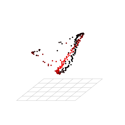
Figure 1: Synthetic data in original and diffusion coordinates

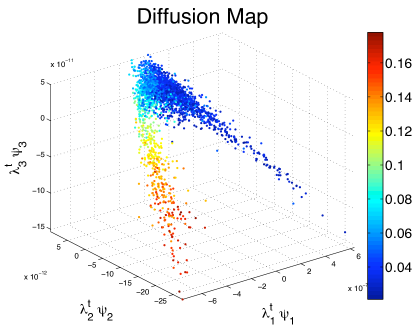
Figure 2: Left: Flux versus wavelength for a typical Sloan Digital Sky Survey (SDSS) galaxy spectrum. Right: Embedding of a sample of 2,793 SDSS galaxy spectra using the first 3 diffusion map coordinates. The color codes for redshift. The reparameterization shows a clear correspondence with variations in redshift, even though redshift was not taken into account in the construction. (Reproduced from Richards et al. (2009))

More generally, the central goal of spectral kernel methods can be described as follows:

Find a transformation $Z=\Psi(X)$ such that the structure of the distribution $P_{Z}$ is simpler than the structure of the distribution $P_{X}$ while preserving key geometric properties of $P_{X}$.

“Simpler” can mean lower dimensional but can be intepreted much more broadly as we shall see.

These new methods of data reparameterization are more flexible than traditional methods such as principal component analysis, clustering and kernel smoothing. Applications of these methods include: manifold learning, (Bickel and Levina, 2004), fast internet web searches (Page et al., 1998), semi-supervised learning for regression and classification (Szummer and Jaakkola, 2001; Lafferty and Wasserman, 2007), inference of arbitrarily shaped clusters, etc. The added flexibility however comes at a price: there are tuning parameters, such as a kernel bandwidth $\varepsilon$, and the dimension $q$ of the embedding that need to be chosen and these parameters often interact in a complicated way. The first step in understanding these tuning parameters is to identify the population quantity these methods are actually estimating, then define an appropriate loss function.

We restrict our discussion to Laplacian-based methods, though the analysis generalizes to other spectral kernel methods. Several authors, including Coifman and Lafon (2006), Belkin and Niyogi (2005), Hein et al. (2005) and Singer (2006), and Giné and Koltchinskii (2006) have studied the convergence of the empirical graph Laplacian to the Laplace-Beltrami operator of a smooth manifold as the sample size $n\rightarrow\infty$ and the kernel bandwidth $\varepsilon\rightarrow 0$. In all these studies, the data are assumed to lie exactly on a Riemannian submanifold in the ambient space $\mathbb{R}^{p}$. Although the theoretical framework is appealing, there are several concerns with this approach: (i) distributions are rarely supported exactly on a manifold, (ii) even in cases where the manifold assumption is approximately reasonable, the bias-variance calculations do not actually take into account stochastic variations about a perfect manifold, (iii) the calculations give no information on how the parameters in the model (such as for example the number of eigenvectors in the embedding) depend on the sample size $n$ and the dimension $p$ when noise is present.

We drop the manifold assumption and instead consider data that are drawn from some general underlying distribution. Recently, other work has taken a similar approach. For example, von Luxburg et al. (2008) study the consistency of spectral clustering. For a fixed kernel bandwidth $\varepsilon$ and in the limit of the sample size $n\rightarrow\infty$, the authors show that the eigenvectors of the graph Laplacian converge to the eigenvectors of certain limit operators. In this paper, we allow $\varepsilon$ to go to 0.

The goals of the paper are to:

1. identify the population quantities being implicitly estimated in Laplacian-based spectral methods,

2. explain how these methods relate to classical kernel smoothing methods,

3. find the appropriate risk and propose an approach to choosing the tuning parameters.

We show that spectral methods are closely related to classical kernel smoothing. This link provides insight into the problem of parameter estimation in Laplacian eigenmaps and spectral clustering. The real power in spectral methods is that they find structure in the data. In particular, they perform connectivity learning, with data reduction and manifold learning being special cases.

Laplacian-based kernel methods essentially use the same smoothing operators as in traditional nonparametric statistics but the end goal is not smoothing. These new kernel methods exploit the fact that the eigenvalues and eigenvectors of local smoothing operators provide information on the underlying geometry of the data.

In this paper, we describe a version of Laplacian-based spectral methods, called diffusion maps. These techniques capture multiscale structure in data by propagating local neighborhood information through a Markov process. Spectral geometry and higher-order connectivity are two new concepts in data analysis. In this paper, we show how these ideas can be incorporated into a traditional statistical framework, and how this connection extends classical techniques to a whole range of new applications. We refer to the resulting method as Spectral Connectivity Analysis (SCA).

2 Review of Spectral Dimension Reduction Methods

The goal of dimensionality reduction is to find a function $\Psi$ that maps our data $X$ from a space $\mathcal{X}$ to a new space $\mathcal{Z}$ where their description is considered to be simpler. Some of the methods naturally lead to an eigen-problem. Below we give some examples.

2.1 Principal Component Analysis and Multidimensional Scaling

Principal component mapping is a simple and popular method for data reduction. In principal component analysis (PCA), one attempts to fit a globally linear model to the data. If $S$ is a set, define

$$R(S)=\mathbb{E}\|X-\pi_{S}X\|^{2}$$ (1)

where $\pi_{S}X$ is the projection of $X$ onto $S$. Finding ${\rm argmin}_{S\in{\cal C}}R(S)$, where ${\cal C}$ is the set of all $q$-dimensional planes, gives a solution that corresponds to the first $q$ eigenvectors of the covariance matrix of $X$.

In principal coordinate analysis, the projections $\pi_{S}x=(z_{1},\ldots,z_{q})$ on these eigenvectors are used as coordinates of the data. This method of reparameterization is also known as classical or metric multidimensional scaling (MDS). The goal here is to find a lower-dimensional embedding of the data that best preserves pairwise Euclidean distances. Assume that $X$ and $Y$ are covariates in $\mathbb{R}^{p}$. One way to measure the discrepancy between the original configuration and its embedding is to compute

$$R(\Psi)=\mathbb{E}\left(d(X,Y)^{2}-\|\Psi(X)-\Psi(Y)\|^{2}\right)=\int\left(d(x,y)^{2}-\|\Psi(x)-\Psi(y)\|^{2}\right)dP(x)dP(y)\ ,$$

where $d(x,y)^{2}=\|x-y\|^{2}$. One can show that amongst all linear projections $\Psi=\pi_{S}$ onto $q$-dimensional subspaces of $\mathbb{R}^{p}$, this quantity is minimized when the data are projected onto their first $q$ principal components (Mardia et al., 1980). Thus, there is a close connection between principal component analysis, which returns the span of a hyperplane, and classical MDS or “principal coordinate analysis”, which returns the new parameterization $\Psi(x)=(z_{1},\ldots,z_{q})$.

The duality between PCA and MDS is also directly apparent in empirical computations: Let $\mathbb{X}$ be an $n\times p$ data matrix, where the rows are observations $x_{i}\in\mathbb{R}^{p}$ centered so that $\frac{1}{n}\sum_{i=1}^{n}x_{i}=0$. The solution to PCA is then given by the principal eigenvectors $\{v_{\ell}\}$ of the $p\times p$ sample covariance matrix $\mathbb{S}=\frac{1}{n}\mathbb{X}^{T}\mathbb{X}$. The solution to the MDS problem, on the other hand, is given by the rescaled eigenvectors of the $n\times n$ Gram or (the positive semi-definite) inner product matrix $\mathbb{K}=\mathbb{X}\mathbb{X}^{T}$, where element $\mathbb{K}(i,j)=\langle x_{i},x_{j}\rangle$. If $\{\lambda_{\ell},u_{\ell}\}$ are the principal eigenvalues and eigenvectors of $\mathbb{K}$, then $\Psi(x_{i})=(\lambda_{1}^{1/2}u_{1}(i),\lambda_{2}^{1/2}u_{2}(i),\ldots)$.

2.2 Non-Linear Methods

For complex data, a linear model may not be adequate. There are a large number of non-linear data reduction methods; some of these are direct generalizations of the PCA projection method. For example, local PCA (Kambhatla and Leen, 1997) partitions the data space into different regions and fits a hyperplane to the data in each partition. In principal curves (Hastie and Stuetzle, 1989), the goal is to minimize a risk of the same form as in Equation 1, but with $S$ representing some class of smooth curves or surfaces.

Among non-linear extensions of PCA and MDS, we also have kernel PCA (Schölkopf et al., 1998) which applies PCA to data $\Phi(X)$ in a higher (possibly infinite) dimensional “feature space”. The kernel PCA method never explicitly computes the map $\Phi$, but instead expresses all calculations in terms of inner products $k(x,y)=\langle\Phi(x),\Phi(y)\rangle$ where the “kernel” $k$ is a symmetric and positive semi-definite function. Common choices include the Gaussian kernel $k(x,y)=\exp\left(-\frac{\|x-y\|^{2}}{4\varepsilon}\right)$ and the polynomial kernel $k(x,y)=\langle x,y\rangle^{r}$, where $r=1$ corresponds to the linear case in Sec. 2.1. As shown in Bengio et al. (2004), the low-dimensional embeddings $\Psi(x)$ used by eigenmap and spectral clustering methods are equivalent to the projections (of $\Phi(x)$ on the principal axes in feature space) computed by the kernel PCA method.

In this paper, we study diffusion maps, a particular spectral embedding technique. Because of the close connection between MDS, kernel PCA and eigenmap techniques, our analysis can be used for other methods a well. Below we start by providing some background on spectral dimension reduction methods from a more traditional graph-theoretic perspective. In the next section we begin our main analysis.

2.2.1 Laplacian eigenmaps and other locality-preserving spectral methods

Most spectral methods take a data-analytic rather than a probabilistic approach to dimension reduction. The usual strategy is to construct an adjacency graph on a given data set and then find the optimal clustering or parameterization of the data that minimizes some empirical locality-preserving objective function on the graph.

For a data set with $n$ observations, we define a graph $G=(V,E)$, where the vertex set $V=\{1,\ldots,n\}$ denotes the observations, and the edge set $E$ represents connections between pairs of observations. Typically, the graph is also associated with a weight matrix $\mathbb{K}$ that reflects the “edge masses” or strengths of the edge connections. A common choice for data in Euclidean space is to start with a Gaussian kernel: Define $\mathbb{K}(u,v)=\exp\left(-\frac{\|x_{u}-x_{v}\|^{2}}{4\varepsilon}\right)$ for all data pairs $(x_{u},x_{v})$ with $(u,v)\in E$, and only include cases where the weights $\mathbb{K}(u,v)$ are above some threshold $\delta$ in the definition of the edge set $E$ .

Consider now a one-dimensional map $f:V\rightarrow\mathbb{R}$ that assigns a real value to each vertex; we will later generalize to the multidimensional case. Many spectral embedding techniques are locality-preserving; e.g. locally linear embedding, Laplacian eigenmaps, Hessian eigenmaps, local tangent space alignment, etc. These methods are special cases of kernel PCA, and all aim at minimizing distortions of the form

$$Q(f)=\sum_{v\in V}Q_{v}(f)$$ (2)

under the constraints that $Q_{M}(f)=1$. Typically, $Q_{v}(f)$ is a symmetric positive semi-definite quadratic form that measures local variations of $f$ around vertex $v$, and $Q_{M}(f)$ is a quadratic form that acts as a normalization for $f$. For Laplacian eigenmaps, for example, the neighborhood structure of $G$ is described in terms of the graph Laplacian matrix

$$\mathbb{L}=\mathbb{M}-\mathbb{K},$$

where $\mathbb{M}=\rm{diag}(\rho_{1},\ldots,\rho_{n})$ is a diagonal matrix with $\rho_{u}=\sum_{v}\mathbb{K}(u,v)$ for the “node mass” or degree of vertex $u$. The goal is to find the map $f$ that minimizes the weighted local distortion

$$Q(f)=f^{T}\mathbb{L}f=\sum_{(u,v)\in E}\mathbb{K}(u,v)\left(f(u)-f(v)\right)^{2}\ \geq\ 0,$$ (3)

under the constraints that

$$Q_{M}(f)=f^{t}\mathbb{M}f=\sum_{v\in V}m_{v}f(v)^{2}=1$$

and (to avoid the trivial solution of a constant function) $f^{T}\mathbb{M}1=0$. Minimizing the distortion in (3) forces $f(u)$ and $f(v)$ to be close if $\mathbb{K}(u,v)$ is large. From standard linear algebra it follows that the optimal embedding is given by the eigenvector of the generalized eigenvalue problem

$$\mathbb{L}f=\mu\mathbb{M}f$$ (4)

with the smallest non-zero eigenvalue.

We can easily extend the discussion to higher dimensions. Let $f_{1},\ldots,f_{q}$ be the $q$ first non-trivial eigenvectors of (4), normalized so that $f_{i}^{T}Mf_{j}=\delta_{ij}$, where $\delta_{ij}$ is Kronecker’s delta function. The map $f:V\rightarrow\mathbb{R}^{q}$, where

$$f=(f_{1},\ldots,f_{q})\ ,$$ (5)

is the Laplacian eigenmap (Belkin and Niyogi, 2003) of $G$ in $q$ dimensions. It is optimal in the sense that it provides the $q$-dimensional embedding that minimizes

$$\sum_{(u,v)\in E}\mathbb{K}(u,v)\|f(u)-f(v)\|^{2}=\sum_{i=1}^{q}f_{i}^{T}\mathbb{L}f_{i}$$ (6)

in the subspace orthogonal to $\mathbb{M}1$, under the constraints that $f_{i}^{T}\mathbb{M}f_{j}=\delta_{ij}$ for $i,j=1,\ldots,q$.

If the data points $x_{u}$ lie on a Riemannian manifold $\mathcal{M}$, and $f:\mathcal{M}\rightarrow\mathbb{R}$ is a twice differentiable function, then the expression in Eq. 3 is the discrete analogue on graphs of $\int_{\mathcal{M}}\|\nabla_{\mathcal{M}}f\|^{2}=-\int_{\mathcal{M}}(\triangle_{\mathcal{M}}f)f$, where $\nabla_{\mathcal{M}}$ and $\triangle_{\mathcal{M}}$, respectively, are the gradient and Laplace-Beltrami operators on the manifold. The solution of $\arg\min_{\|f\|=1}\int_{\mathcal{M}}\|\nabla_{\mathcal{M}}f\|^{2}$ is given by the eigenvectors of the Laplace-Beltrami operator $\triangle_{\mathcal{M}}$. To give a theoretical justification for Laplacian-based spectral methods, several authors have derived results for the convergence of the graph Laplacian of a point cloud to the Laplace-Beltrami operator under the manifold assumption; see Belkin and Niyogi (2005); Coifman and Lafon (2006); Singer (2006); Giné and Koltchinskii (2006).

2.2.2 Laplacian-based methods with an explicit metric

Diffusion mapping is an MDS technique that belongs to the family of Laplacian-based spectral methods. The original scheme was introduced in the thesis work by Lafon (2004) and in Coifman et al. (2005a, b). See also independent work by Fouss et al. (2005) for a similar technique called Euclidean commute time (ECT) maps. In this paper, we will describe a slightly modified version of diffusion maps that appeared in (Coifman and Lafon, 2006; Lafon and Lee, 2006) .

The starting point of the diffusion framework is to introduce a distance metric that reflects the higher-order connectivity of the data. This is effectively done by defining a diffusion process or random walk on the data.

As before, we here describe a graph approach where the nodes of the graph represent the observations in the data set. Assuming non-negative weights $\mathbb{K}$ and a degree matrix $\mathbb{M}$, we define a row-stochastic matrix $\mathbb{A}=\mathbb{M}^{-1}\mathbb{K}$. We then imagine a random walk on the graph $G=(V,E)$ where $\mathbb{A}$ is the transition matrix, and element $\mathbb{A}(u,v)$ corresponds to the probability of reaching node $v$ from $u$ in one step. Now if $\mathbb{A}^{m}$ is the $m^{\rm th}$ matrix power of $\mathbb{A}$, then element $\mathbb{A}^{m}(u,v)$ can be interpreted as the probability of transition from $u$ to $v$ in $m$ steps. By increasing $m$, we are running the Markov chain forward in time, thereby describing larger scale structures in the data set. Under certain conditions on $\mathbb{K}$, the Markov chain has a unique stationary distribution $s(v)=\rho(v)/{\sum_{u\in V}\rho(u)}$.

We define the diffusion distance between nodes $u$ and $v$ as a weighted $L^{2}$ distance between the two distributions $\mathbb{A}^{m}(u,\cdot)$ and $\mathbb{A}^{m}(v,\cdot)$,

$$D_{m}(u,v)^{2}=\sum_{k\in V}\frac{\left(\mathbb{A}^{m}(u,k)-\mathbb{A}^{m}(v,k)\right)^{2}}{s(k)}.$$

This quantity captures the higher-order connectivity of the data at a scale $m$ and is very robust to noise since it integrates multiple-step, multiple-path connections between points. The distance $D_{m}(u,v)^{2}$ is small when $A^{m}(u,v)$ is large, or when there are many paths between nodes $u$ and $v$ in the graph.

As in multidimensional scaling, the ultimate goal is to find an embedding of the data where Euclidean distances reflect similarities between points. In classical MDS, one attempts to preserve the original Euclidean distances $d^{2}(u,v)=\|x_{u}-x_{v}\|^{2}$ between points. In diffusion maps, the goal is to approximate diffusion distances $D_{m}^{2}(u,v)$. One can show (see appendix) that the optimal embedding in $q$ dimensions is given by a “diffusion map” $\Psi_{m}$, where the coordinates of the data are the (rescaled) right eigenvectors of the Markov matrix $\mathbb{A}$. In fact, assuming the kernel matrix $\mathbb{K}$ is positive semi-definite, we have that

$$v\in V\ \mapsto\ \Psi_{m}(v)=(\lambda_{1}^{m}\psi_{1}(v),\lambda_{2}^{m}\psi_{2}(v),\ldots,\lambda_{q}^{m}\psi_{q}(v))\in\mathbb{R}^{q}\ ,$$

where $\{\psi_{\ell}\}_{\ell\geq 0}$ are the principal eigenvectors of $\mathbb{A}$ and the eigenvalues $\lambda_{0}=1\geq\lambda_{1}\geq\ldots 0$. This solution is, up to a rescaling, the same as the solution of Laplacian eigenmaps and spectral clustering, since

$$\ \ \mathbb{L}\psi=\mu\mathbb{M}\psi\ \ \Leftrightarrow\ \ \mathbb{A}\psi=\lambda\psi\ .$$

for $\lambda=1-\mu$ and $\mathbb{L}=\mathbb{M}-\mathbb{K}$. The diffusion framework provides a link between Laplacian-based spectral methods, MDS and kernel PCA, and can also be generalized to multiscale geometries (Coifman et al., 2005b; Coifman and Maggioni, 2006).

Remark 1

The link to MDS and kernel PCA is even more explicit in the original version of diffusion maps (Coifman et al., 2005a), which is based on the symmetric (positive semi-definite) kernel matrix $\widetilde{\mathbb{A}}^{m}=\mathbb{M}^{1/2}\mathbb{A}^{m}\mathbb{M}^{-1/2}=\mathbb{I}-\mathbb{M}^{-1/2}\mathbb{L}\mathbb{M}^{-1/2}$, and the metric $D_{m}^{2}(u,v)=\widetilde{\mathbb{A}}^{m}(u,u)+\widetilde{\mathbb{A}}^{m}(v,v)-2\widetilde{\mathbb{A}}^{m}(u,v)$ induced by this kernel. In classical MDS and linear PCA, the analogue is a positive semi-definite kernel matrix $\mathbb{K}$, where $\mathbb{K}(u,v)=\langle x_{u},x_{v}\rangle$, and Euclidean distances $d^{2}(u,v)=\|x_{u}-x_{v}\|^{2}=\mathbb{K}(u,u)+\mathbb{K}(v,v)-2\mathbb{K}(u,v)$. In both cases, the data are parameterized by the rescaled principal eigenvectors $(\lambda_{1}^{1/2}\phi_{1},\lambda_{2}^{1/2}\phi_{2},\ldots)$ of the kernel matrix associated with the metric.

3 Diffusion Maps

The diffusion map creates a distribution-sensitive reparameterization. We will study the method under the assumption that the data are drawn from an underlying distribution. We begin by introducing a Markov chain that plays an important role in the definition of the diffusion map.

3.1 A Discrete-Time Markov Chain

Definitions. Suppose that the data $X_{1},\ldots,X_{n}$ are drawn from some underlying distribution $P$ with compact support ${\cal X}\subset\mathbb{R}^{d}$. We assume $P$ has a density $p$ with respect to Lebesgue measure $\mu$. Let

$$k_{\varepsilon}(x,y)=\frac{1}{(4\pi\varepsilon)^{d/2}}\exp\left(-\frac{\|x-y\|^{2}}{4\varepsilon}\right)$$ (7)

denote the Gaussian kernel with bandwidth $h=\sqrt{2\varepsilon}$. We write the bandwidth in terms of $\varepsilon$ instead of $h$ because $\varepsilon$ is more natural for our purposes. Consider the Markov chain with transition kernel $\Omega_{\varepsilon}(x,\cdot)$ defined by

$$\Omega_{\varepsilon}(x,A)=\mathbb{P}(x\to A)=\frac{\int_{A}k_{\varepsilon}(x,y)dP(y)}{\int k_{\varepsilon}(x,y)dP(y)}=\frac{\int_{A}k_{\varepsilon}(x,y)dP(y)}{p_{\varepsilon}(x)}$$ (8)

where $p_{\varepsilon}(x)=\int k_{\varepsilon}(x,y)dP(y)$.

Starting at $x$, this chain moves to points $y$ close to $x$, giving preference to points with high density $p(y)$. In a sense, this chain measures the connectivity of the sample space relative to $p$. The stationary distribution $S_{\varepsilon}$ is given by

$$S_{\varepsilon}(A)=\frac{\int_{A}p_{\varepsilon}(x)dP(x)}{\int p_{\varepsilon}(x)dP(x)}$$

and

$$S_{\varepsilon}(A)\to\frac{\int_{A}p(x)dP(x)}{\int p(x)dP(x)}\ \ \ {\rm as}\ \varepsilon\to 0.$$

Define the densities

$$\omega_{\varepsilon}(x,y) = \frac{d\Omega_{\varepsilon}}{d\mu}(x,y)=\frac{k_{\varepsilon}(x,y)p(y)}{p_{\epsilon}(x)}$$

$$a_{\varepsilon}(x,y) = \frac{d\Omega_{\varepsilon}}{dP}(x,y)=\frac{k_{\varepsilon}(x,y)}{p_{\epsilon}(x)}.$$

The diffusion operator $A_{\varepsilon}$—which maps a function $f$ to a new function $A_{\varepsilon}f$— is defined by

$$A_{\varepsilon}f(x)=\int a_{\varepsilon}(x,y)f(y)dP(y)=\frac{\int k_{\varepsilon}(x,y)f(y)dP(y)}{\int k_{\varepsilon}(x,y)dP(y)}.$$ (9)

We normalize the eigenfunctions $\{\psi_{\varepsilon,0},\psi_{\varepsilon,1},\ldots\}$ of $A_{\varepsilon}$ by

$$\int\psi_{\varepsilon,\ell}^{2}(x)s_{\varepsilon}(x)dP(x)=1,$$

where

$$s_{\varepsilon}(x)=\frac{p_{\varepsilon}(x)}{\int p_{\varepsilon}(y)dP(y)}$$

is the density of the stationary distribution with respect to $P$. The first eigenfunction of the operator $A_{\varepsilon}$ is $\psi_{\varepsilon,0}(x)=1$ with eigenvalue $\lambda_{\varepsilon,0}=1$. In general, the eigenfunctions have the following interpretation: $\psi_{\varepsilon,j}$ is the smoothest function relative to $p$, subject to being orthogonal to $\psi_{\varepsilon,i}$, $i<j$. The eigenfunctions form an efficient basis for expressing smoothness, relative to $p$. If a distribution has a few well defined clusters then the first few eigenfunctions tend to behave like indicator functions (or combinations of indicator functions) for those clusters. The rest of the eigenfunctions provide smooth basis functions within each cluster. These smooth functions are Fourier-like. Indeed, the uniform distribution on the circle yields the usual Fourier basis. Figure 3 shows a density which is a mixture of two Gaussians. Also shown are the eigenvalues and the first 4 eigenfunctions which illustrate these features.

Figure 3: A mixture of two Gaussians. Density, eigenvalues, and first four eigenfunctions.

Denote the $m$-step transition measure by $\Omega_{\varepsilon,m}(x,\cdot)$. Let $A_{\varepsilon,m}$ be the corresponding diffusion operator which can be written as

$$A_{\varepsilon,m}f(x)=\int a_{\varepsilon,m}(x,y)f(y)dP(y)$$

where $a_{\varepsilon,m}(x,y)=d\Omega_{\varepsilon,m}/dP$.

Define the empirical operator $\widehat{A}_{\varepsilon}$ by

$$\widehat{A}_{\varepsilon}f(x)=\frac{\sum_{i=1}^{n}k_{\varepsilon}(x,X_{i})f(X_{i})}{\sum_{i=1}^{n}k_{\varepsilon}(x,X_{i})}=\int\widehat{a}_{\varepsilon}(x,y)f(y)d\widehat{P}_{n}(y)$$ (10)

where $\widehat{P}_{n}$ denotes the empirical distribution, $\widehat{a}_{\varepsilon}(x,y)={k_{\varepsilon}(x,y)}/{\widehat{p}_{\varepsilon}(x)}$ and

$$\widehat{p}_{\varepsilon}(x)=\int k_{\varepsilon}(x,y)d\widehat{P}_{n}(y)=\frac{1}{n}\sum_{i=1}^{n}k_{\varepsilon}(x,X_{i})$$ (11)

is the kernel density estimator. Let $\widehat{A}_{\varepsilon,m}$ be the corresponding $m$-step operator. Let $\widehat{\psi}_{\varepsilon,\ell}$ denote the eigenvectors of the matrix $\mathbb{A}_{\varepsilon}$ where $\mathbb{A}_{\varepsilon}(j,k)=k_{\varepsilon}(X_{j},X_{k})/\widehat{p}_{\varepsilon}(X_{j})$. These eigenvectors are estimates of $\psi_{\ell}$ at the observed values $X_{1},\ldots,X_{n}$. The function $\psi_{\ell}(x)$ can be estimated at values of $x$ not corresponding to one of the $X_{i}$’s by kernel smoothing as follows. The eigenfunction-eigenvalue equation $\lambda_{\varepsilon,\ell}\psi_{\varepsilon,\ell}=A_{\varepsilon}\psi_{\varepsilon,\ell}$ can be rearranged as

$$\psi_{\varepsilon,\ell}(x)=\frac{A_{\varepsilon}\psi_{\varepsilon,\ell}}{\lambda_{\varepsilon,\ell}}=\frac{\int k_{\varepsilon}(x,y)\psi_{\varepsilon,\ell}(y)dP(y)}{\lambda_{\varepsilon,\ell}\int k_{\varepsilon}(x,y)dP(y)}$$ (12)

suggesting the estimate

$$\widehat{\psi}_{\varepsilon,\ell}(x)=\frac{\sum_{i}k_{\varepsilon}(x,X_{i})\widehat{\psi}_{\varepsilon,\ell}(X_{i})}{\widehat{\lambda}_{\varepsilon,\ell}\sum_{i}k_{\varepsilon}(x,X_{i})}$$ (13)

which is known in the applied mathematics literature as the Nyström approximation.

Interpretation. The diffusion operators are averaging operators. Equation (9) arises in nonparametric regression. If we are given regression data $Y_{i}=f(X_{i})+\epsilon_{i}$, $i=1,\ldots,n$, then the kernel regression estimator of $f$ is

$$\widehat{f}(x)=\frac{\frac{1}{n}\sum_{i=1}^{n}Y_{i}k_{\varepsilon}(x,X_{i})}{\frac{1}{n}\sum_{i=1}^{n}k_{\varepsilon}(x,X_{i})}.$$ (14)

Replacing the sample averages in (14) with their population averages yields (9). One may then wonder: in what way spectral smoothing is different from traditional nonparametric smoothing? There are at least three differences:

1. Estimating $A_{\varepsilon}$ is an unsupervised problem, that is, there are no responses $Y_{i}$. (But see Section 7 for applications to supervised problems.)

2. In spectral methods, smoothing is not the end goal. The main objective is finding structure in the data. The eigenvalues and eigenvectors of $\widehat{A}_{\varepsilon}$ provide information on the intrinsic geometry of the data and can be used to parameterize the data.

3. In spectral smoothing, we are interested in $\widehat{A}_{\varepsilon,m}$ for $m\geq 1$. The value $m=1$ leads to a local analysis of the nearest-neighbor structure — this part is equivalent to classical smoothing. Powers $m>1$, however, takes higher-order structure into account.

The concept of connectivity is new in nonparametric statistics and is perhaps best explained in terms of stochastic processes. Introduce the forward Markov operator

$$M_{\varepsilon}g(x)=\int_{\mathcal{X}}a_{\varepsilon}(y,x)g(y)dP(y)$$ (15)

and its $m$-step version $M_{\varepsilon,m}$. The first eigenfunction of $M_{\varepsilon}$ is $\varphi_{\varepsilon,0}(x)=s_{\varepsilon}(x)$, the density of the stationary distribution. In general,

$$\varphi_{\varepsilon,\ell}=s_{\varepsilon}(x)\psi_{\varepsilon,\ell}(x).$$

The averaging operator $A$ and the Markov operator $M$ and (and hence also the iterates $A_{\varepsilon,m}$ and $M_{\varepsilon,m}$) are adjoint under the inner product $\langle f,g\rangle=\int_{\mathcal{X}}f(x)g(x)dP(x)$, i.e. $\langle A_{\varepsilon}f,g\rangle=\langle f,M_{\varepsilon}g\rangle$. By comparing (7) and the heat kernel of a continuous-time diffusion process (see equation (3.28) in  Grigor’yan (2006)), we identify the time step of the discrete system as $t=m\varepsilon$.

The Markov operator $M_{\varepsilon}=A^{*}_{\varepsilon}$ maps measures into measures. That is, let $L^{1}_{P}(\mathcal{X})=\{g:\ g(y)\geq 0,\int g(y)dP(y)=1\}$. Then $g\in L^{1}_{P}(\mathcal{X})$ implies that $M_{\varepsilon,m}g\in L^{1}_{P}(\mathcal{X})$. In particular, if $\varphi$ is the probability density at time $t=0$, then $M_{\varepsilon,m}\varphi$ is the probability density after $m$ steps. The averaging operator $A_{\varepsilon}$ maps observables into observables. Its action is to compute conditional expectations. If $f\in L^{\infty}_{P}(\mathcal{X})$ is the test function (observable) at $t=0$, then $A_{\varepsilon,m}f\in L^{\infty}_{P}(\mathcal{X})$ is the average of the function after $m$ steps, i.e. at a time comparable to $t=m\varepsilon$ for a continuous time system.

3.2 Continuous Time

Under appropriate regularity conditions, the eigenfunctions $\{\psi_{\varepsilon,\ell}\}$ converge to a set of functions $\{\psi_{\ell}\}$ as $\varepsilon\to 0$. These limiting eigenfunctions correspond to some operator. In this section we identify this operator. The key is to consider the Markov chain with infinitesimal transitions. In physics, local infinitesimal transitions of a system lead to global macroscopic descriptions by integration. Here we use the same tools (infinitesimal operators, generators, exponential maps, etc) to extend short-time transitions to larger times.

Define the operator

$$G_{\varepsilon}f(x)=\frac{1}{\varepsilon}\left(\int_{\mathcal{X}}a_{\varepsilon}(x,y)f(y)dP(y)-f(x)\right)\ .$$ (16)

Assume that the limit

$$\mathbf{G}f=\lim_{\varepsilon\to 0}G_{\varepsilon}f=\lim_{\varepsilon\rightarrow 0}\frac{A_{\varepsilon}f-f}{\varepsilon}$$ (17)

exists for all functions $f$ in some appropriately defined space of functions ${\cal F}$. The operator $\mathbf{G}$ is known as the infinitesimal generator. A Taylor expansion shows that

$$\mathbf{G}=-\triangle+\frac{\nabla p}{p}$$ (18)

for smooth functions where $\triangle$ is the Laplacian and $\nabla$ is the gradient. Indeed, $G_{\varepsilon}f=-\triangle f+\frac{\nabla p}{p}+O(\varepsilon)$ which is precisely the bias for kernel regression.

Remark 2

In kernel regression smoothing, the term $\nabla p/p$ is considered an undesirable extra bias, called design bias (Fan (1993)). In regression it is removed by using local linear smoothing which is asymptotically equivalent to replacing the Gaussian kernel $k_{\varepsilon}$ with a bias-reducing kernel $k_{\varepsilon}^{*}$. In this case, $\mathbf{G}=-\Delta$.

For $\ell>0$ define

$$\nu_{\varepsilon,\ell}^{2}=\frac{1-\lambda_{\varepsilon,\ell}}{\varepsilon}\ \ \ {\rm and}\ \ \ \nu_{\ell}^{2}=\lim_{\varepsilon\to 0}\nu_{\varepsilon,\ell}^{2}.$$ (19)

The eigenvalues and eigenvectors of $G_{\varepsilon}$ are $-\nu_{\varepsilon,\ell}^{2}$ and $\psi_{\varepsilon,\ell}$ while the eigenvalues and eigenvectors of the generator $\mathbf{G}$ are $-\nu_{\ell}^{2}$ and $\psi_{\ell}$. Also, $\psi_{\varepsilon,\ell}\approx\psi_{\ell}$.

Let $\mathbf{A}_{t}=\lim_{\varepsilon\rightarrow 0}A_{\varepsilon,t/\varepsilon}$. From (16) and (17), it follows that

$$\mathbf{A}_{t}\equiv\lim_{\varepsilon\rightarrow 0}A_{\varepsilon,t/\varepsilon}=\lim_{\varepsilon\rightarrow 0}(I+\varepsilon G_{\varepsilon})^{t/\varepsilon}=\lim_{\varepsilon\rightarrow 0}(I+\varepsilon\mathbf{G})^{t/\varepsilon}=e^{\mathbf{G}t}.$$ (20)

The family $\{\mathbf{A}_{t}\}_{t\geq 0}$ defines a continuous semigroup of operators (Lasota and Mackey, 1994). The notation is summarized in Table 1.

Table 1: Summary of notation

Operator	Eigenfunctions	Eigenvalues
$A_{\varepsilon}f(\cdot)=\frac{\int k_{\varepsilon}(\cdot,y)f(y)dP(y)}{\int k_{\varepsilon}(\cdot,y)dP(y)}$	$\psi_{\varepsilon,\ell}$	$\lambda_{\varepsilon,\ell}$
$\mathbf{G}=\lim_{\varepsilon\to 0}\frac{A_{\varepsilon}-I}{\varepsilon}$	$\psi_{\ell}$	$-\nu_{\ell}^{2}=\lim_{\varepsilon\to 0}\frac{\lambda_{\varepsilon,\ell}-1}{\varepsilon}$
$\mathbf{A}_{t}=e^{t\mathbf{G}}=\sum_{\ell=0}^{\infty}e^{-\nu_{\ell}^{2}t}\Pi_{\ell}$	$\psi_{\ell}$	$e^{-t\nu_{\ell}^{2}}=\lim_{\varepsilon\rightarrow 0}\lambda_{\varepsilon,\ell}^{t/\varepsilon}$
$\mathbf{A}_{t}$ $=\lim_{\varepsilon\to 0}A_{\epsilon,t/\varepsilon}$

One of our goals is to find the bandwidth $\varepsilon$ so that $\widehat{A}_{\varepsilon,t/\varepsilon}$ is a good estimate of $\mathbf{A}_{t}$. We show that this is a well-defined problem. Related work on manifold learning, on the other hand, only discusses the convergence properties of the graph Laplacian to the Laplace-Beltrami operator, i.e. the generators of the diffusion. Estimating the generator $\mathbf{G}$, however, does not answer questions regarding the optimal choice of the number of eigenvectors, the number of groups in spectral clustering etc.

We can express the diffusion in terms of its eigenfunctions. Mercer’s theorem gives the biorthogonal decomposition

$$a_{\varepsilon}(x,y) = \sum_{\ell\geq 0}\lambda_{\varepsilon,\ell}\psi_{\varepsilon,\ell}(x)\varphi_{\varepsilon,\ell}(y),$$ (21)

$$a_{\varepsilon,t/\varepsilon}(x,y) = \sum_{\ell\geq 0}\lambda_{\varepsilon,\ell}^{t/\varepsilon}\psi_{\varepsilon,\ell}(x)\varphi_{\varepsilon,\ell}(y)$$ (22)

where $\psi_{\varepsilon,\ell}$ are the eigenvectors of $A_{\varepsilon}$, and $\varphi_{\varepsilon,\ell}$ are the eigenvectors of its adjoint $M_{\varepsilon}$. The details are given in Appendix 8.1. From (16), it follows that the eigenvalues $\lambda_{\varepsilon,\ell}=1-\varepsilon\nu_{\varepsilon,\ell}^{2}$. The averaging operator $A_{\varepsilon}$ and its generator $G_{\varepsilon}$ have the same eigenvectors. Inserting (21) into (9) and recalling that $\varphi_{\varepsilon,\ell}(x)=s_{\varepsilon}(x)\psi_{\varepsilon,\ell}(x)$, gives

$$A_{\varepsilon}f(x) = \sum_{\ell\geq 0}\lambda_{\varepsilon,\ell}\psi_{\varepsilon,\ell}(x)\int_{\mathcal{X}}\varphi_{\varepsilon,\ell}(y)f(y)dP(y)$$

$$= \sum_{\ell\geq 0}\lambda_{\varepsilon,\ell}\psi_{\varepsilon,\ell}(x)\int_{\mathcal{X}}\psi_{\varepsilon,\ell}(y)f(y)s_{\varepsilon}(y)dP(y)$$

$$= \sum_{\ell\geq 0}\lambda_{\varepsilon,\ell}\psi_{\varepsilon,\ell}(x)\langle\psi_{\varepsilon,\ell},f\rangle_{\varepsilon}=\sum_{\ell\geq 0}\lambda_{\varepsilon,\ell}\ \Pi_{\varepsilon,\ell}f(x)$$

where $\langle f,g\rangle_{\varepsilon}\equiv\int_{\mathcal{X}}f(y)g(y)s_{\varepsilon}(y)dP(y)$ and $\Pi_{\varepsilon,\ell}$ is the weighted orthogonal projector on the eigenspace spanned by $\psi_{\varepsilon,\ell}$. Thus,

$$A_{\varepsilon,t/\varepsilon}=\sum_{\ell\geq 0}\lambda_{\varepsilon,\ell}^{t/\varepsilon}\Pi_{\varepsilon,\ell}.$$ (23)

Similarly, assuming the limit in (20) exists,

$$\mathbf{A}_{t}=\sum_{\ell\geq 0}e^{-\nu_{\ell}^{2}t}\Pi_{\ell}$$ (24)

where $\Pi_{\ell}$ is the weighted orthogonal projector on the eigenspace corresponding to the eigenfunction $\psi_{\ell}$ of $\mathbf{G}$. Weyl’s theorem (Stewart (1991)) gives

$$\sup_{\ell}|e^{-\nu_{\ell}^{2}t}-\lambda_{\varepsilon,\ell}^{t/\varepsilon}|\leq\|A_{\varepsilon,t/\varepsilon}-e^{\mathbf{G}t}\|=t\varepsilon+O(\varepsilon^{2}),$$ (25)

$$\lim_{\varepsilon\rightarrow 0}\lambda_{\varepsilon,\ell}^{t/\varepsilon}=e^{-\nu_{\ell}^{2}t},\ \ \ \lim_{\varepsilon\rightarrow 0}\Pi_{\varepsilon,\ell}=\Pi_{\ell}.$$

Note that $\{\psi_{\ell}\}$ is an orthonormal basis with respect to the inner product

$$\langle f,g\rangle_{\varepsilon}=\int f(x)g(x)s_{\varepsilon}(x)dP(x)$$

while $\{\varphi_{\ell}\}$ is an orthonormal basis with respect to the inner product

$$\langle f,g\rangle_{1/\varepsilon}=\int\frac{f(x)g(x)}{s_{\varepsilon}(x)}dP(x).$$

Equation (24) implies that to estimate the action of the limiting operator $\mathbf{A}_{t}$ at a given time $t>0$, we need the dominant eigenvalues and eigenvectors of the generator $\mathbf{G}$. Finally, we also define the limiting transition density

$$\mathbf{a}_{t}(x,y)=\lim_{\varepsilon\to 0}a_{\varepsilon,t/\varepsilon}(x,y).$$ (27)

As $t\to 0$, $\mathbf{a}_{t}(x,y)$ converges to a point mass at $x$; as $t\to\infty$, $\mathbf{a}_{t}(x,y)$ converges to $p(y)$.

Remark 3

There is an important difference between estimating $\mathbf{A}_{t}$ and $\mathbf{G}$: the diffusion operator $\mathbf{A}_{t}$ is a compact operator, while the generator $\mathbf{G}$ is not even a bounded operator. Consider, for example, the Laplacian on a circle $S^{1}$ (Rosenberg, 1997). The eigenfunctions of $\mathbf{G}$ and $\mathbf{A}_{t}$ are here the Fourier basis functions $e^{i\ell x}$ where $\ell=0,\pm 1,\pm 2,\ldots$. The heat operator $e^{-t\Delta}$ is a compact operator. Its eigenvalues are $e^{-\ell^{2}t}(t>0)$ which are clearly bounded above and go to zero. The Laplace-Beltrami operator $\Delta$, on the other hand, has eigenvalues $n^{2}$ which are unbounded.

We will consider some examples in Section 6 but let us first illustrate the definitions for a one-dimensional distribution with multiscale structure.

Example 1

Suppose that $P$ is a mixture of three Gaussians. Figure 4 shows the density $p$. The left column of Figure 5 shows $\Omega_{t}$ for increasing $t$. The right column shows a fixed row of $\Omega_{t}$, namely $\omega_{t}(x,\cdot)$ for a fixed $x$ indicated by the horizontal line. The density $\omega_{t}(x,\cdot)$ starts out concentrated near $x$. As $t$ increases, it begins to spread out. It becomes bimodal at $t=1$ indicating that the two closer clusters have merged. Eventually, the density has three modes (indicating a single cluster) at $t=10$, and then resembles $p$ when $t=1000$ since $\omega_{t}(x,\cdot)\to p^{2}(\cdot)/\int p^{2}(u)du$ as $t\rightarrow\infty$.

Figure 4: The density $p$ for Example 1.

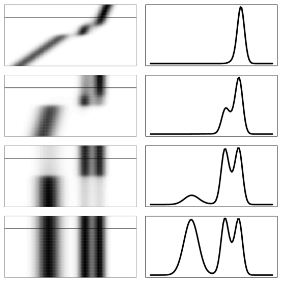
Figure 5: Example 1. Left column: $\omega_{t}(x,y)$ for $t=.1,1,10,1000$. Right column, $\omega_{t}(x,y)$ for a fixed $x$.

3.3 Comparing $\varepsilon$ and $t$

The parameters $t$ and $\varepsilon$ are both related to smoothing but they are quite different. The parameter $t$ is part of the population quantity being estimated and controls the scale of the analysis. Hence, the choice of $t$ is often determined by the problem at hand. The parameter $\varepsilon$ is a smoothing parameter for estimating the population quantity from data. As $n\rightarrow\infty$, we let $\varepsilon_{n}\rightarrow 0$ for more accurate estimates. The following two examples illustrate the differences of smoothing in data when using $\varepsilon$ or $t$.

Example 2

Consider a fixed test function $f$. Define

$${\cal A}=\Biggl{\{}g=A_{\varepsilon}f:\ \ 0\leq\varepsilon\leq\infty\Biggr{\}}\ \ \ {\rm and}\ \ \ {\cal A}^{*}=\Biggl{\{}g=\mathbf{A}_{t}f:\ \ 0\leq t\leq\infty\Biggr{\}}.$$

Let

$$P=\frac{1}{2}\delta_{0}+\frac{1}{2}\delta_{1}$$

where $\delta_{c}$ denotes a point mass distribution at $c$. If $f$ is any continuous functions then both $A_{\varepsilon}$ and $\mathbf{A}_{t}$ depend only on the two values $f(0)$ and $f(1)$ which we will assume are distinct.

Now

$$A_{\varepsilon}f(x)=\frac{k_{\varepsilon}(x,0)f(0)+k_{\varepsilon}(x,1)f(1)}{k_{\varepsilon}(x,0)+k_{\varepsilon}(x,1)}.$$

In particular

$$A_{0}f(x)=\left\{\begin{array}[]{ll}f(0)&x<1/2\\ f(1)&x>1/2.\end{array}\right.$$

and $A_{\infty}f(x)=c$ for all $x$ where $c=(f(0)+f(1))/2$. For $0<\varepsilon<\infty$, $A_{\varepsilon}f(x)$ is a smooth monotone function; see Figure 6.

In contrast,

$$\mathbf{A}_{t}f(x)=\left\{\begin{array}[]{ll}f(0)&x<1/2\\ f(1)&x>1/2\end{array}\right.$$

for all values of $t$. In other words, $\mathbf{A}_{t}f(x)=A_{0}f(x)$ for all $t$. The reason is that $\mathbf{A}_{t}$ has two eigenfunctions: $\psi_{0}(x)=1$ and $\psi_{1}(x)=I(x>1/2)-I(x<1/2)$ (assuming the normalization $\int\psi^{2}(x)dP(x)=1$.) The eigenvalues are $\lambda_{0}=\lambda_{1}=1$. Hence, $\nu_{0}=\nu_{1}=0$ and so

$$\mathbf{A}_{t}=\Pi_{0}+\Pi_{1}$$

where $\Pi_{0}$ projects onto $\psi_{0}$ and $\Pi_{1}$ projects onto $\psi_{1}$. The step function behavior of $\mathbf{A}_{t}$ reflects the lack of connectivity of $P$.

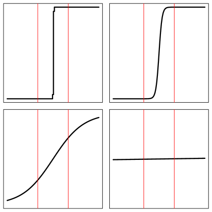
Figure 6: $A_{\varepsilon}f$ for increasing values of $\varepsilon$. The function $\mathbf{A}_{t}f$ corresponds to the top left plot and does not change as $t$ changes.

Example 3

Assume that the distribution is supported along two parallel lines of length $\pi$ at $v=0$ and $v=1$, respectively. The probability measure is

$$P=\frac{1}{2}U_{0}+\frac{1}{2}U_{1}$$

where $U_{0}$ is uniform on $\{(0,x):\ 0\leq x\leq\pi\}$ and $U_{1}$ is uniform on $\{(1,x):\ 0\leq x\leq\pi\}$. Consider a fixed test function $f$. We have that

$$A_{\varepsilon}f(x) = \int\ell_{\varepsilon}(x,y)f(y)dy$$

$$\mathbf{A}_{t}f(x) = \int\mathbf{\ell}_{t}(x,y)f(y)dy\ ,$$

where the weights $\ell_{\varepsilon}(x,y)=\frac{k_{\varepsilon}(x,y)p(y)}{p_{\varepsilon}(x)}$ and $\ell_{t}(x,y)=\mathbf{a}_{t}(x,y)p(y)=\lim_{\varepsilon\to 0}a_{\varepsilon,t/\varepsilon}(x,y)p(y)$  .

Let $x=(0,0)$ and $y=(u,v)$. Figure 7 shows how the weights $\ell_{\varepsilon}(x,y)$ change with the parameter $\varepsilon$. When $\varepsilon$ is small, $A_{\varepsilon}f(x)$ will only depend on the values of $f$ close to the origin along the line at $v=0$. However, with increasing $\varepsilon$, smoothing will also involve function values further from the origin, including values along the parallel line at $v=1$, as indicated by the red dashed curves in the figure.

Figure 7: $\ell_{\varepsilon}(x,y)$ for $x=(0,0)$, $y=(u,v)$ and $\varepsilon=0.01,0.1,1,10$.

In contrast, for $x=(0,0)$, $\mathbf{A}_{t}f(x)$ only depends on values of $f$ in the same connected set as $x$, i.e. function values along the line at $v=0$, regardless of $t$. Figure 8 illustrates how the weights $\ell_{t}(x,y)$ change as the parameter $t$ increases. Smoothing by $t$ reflects the connectivity of the data. In particular, there is no mixing of values of $f$ from disconnected sets.

Figure 8: $\ell_{t}(x,y)$ for $x=(0,0)$, $y=(u,v)$ and $t=0.01,0.1,1,10$.

4 Diffusion Distance

The diffusion distance is another quantity that captures the underlying geometry.

4.1 Definition

For an $m$-step Markov chain, the diffusion distances are defined by

$$D_{\varepsilon,m}^{2}(x,z)=\int\frac{(a_{\varepsilon,m}(x,u)-a_{\varepsilon,m}(z,u))^{2}}{s_{\varepsilon}(u)}dP(u)$$

for $m=1,2,\ldots$. It can be shown (see appendix) that

$$D_{\varepsilon,m}^{2}(x,z)=\sum_{\ell\geq 0}\lambda_{\varepsilon,\ell}^{2m}(\psi_{\varepsilon,\ell}(x)-\psi_{\varepsilon,\ell}(z))^{2}.$$ (28)

Following the same arguments as before we deduce that the corresponding population quantity is

$$\mathbf{D}_{t}^{2}(x,z)=\sum_{\ell\geq 0}e^{-2\nu_{\ell}^{2}t}(\psi_{\ell}(x)-\psi_{\ell}(z))^{2}.$$ (29)

Now we compare diffusion distance to two other distances that have been used recently: geodesic distance and density distance.

4.2 Geodesic Distance

The geodesic distance, or the shortest path, is a very intuitive way of measuring the distance between two points in a set. Some manifold learning algorithms, such as Isomap (Tenenbaum et al., 2000), rely on being able to estimate the geodesic distance on a manifold given data in $\mathbb{R}^{p}$. The idea is to construct a graph $G$ on pairs of points at a distance less than a given threshold $\delta$, and define a graph distance

$$d_{G}(A,B)=\min_{\pi}\left(\|x_{0}-x_{1}\|+\ldots+\|x_{m-1}-x_{m}\|\right)$$

where $\pi=(x_{0},\ldots,x_{m})$ varies over all paths along the edges of $G$ connecting the points $A=x_{0}$ and $B=x_{m}$. Multidimensional scaling is then used to find a low-dimensional embedding of the data that best preserves these distances.

Under the assumption that the data lie exactly on a smooth manifold $\mathcal{M}$, Bernstein et al. (2000) have shown that the graph distance $d_{G}(A,B)$ converges to the geodesic manifold metric

$$d_{\mathcal{M}}(A,B)=\inf\{\mathrm{length}(\gamma)\},$$

where $\gamma$ varies over the set of smooth arcs connecting $A$ and $B$ in $\mathcal{M}$. Beyond this ideal situation, little is known about the statistical properties of the graph distance. Here we show by two examples that the geodesic (graph) distance is inconsistent if the support of the distribution is not exactly on a manifold.

Consider a one-dimensional spiral in a plane:

$$\left\{\begin{array}[]{ccc}x&=&t^{a}\cos(bt)\\ y&=&t^{a}\sin(bt)\end{array}\right.$$

where $a=0.8$ and $b=10$. The geodesic manifold distance $d_{\mathcal{M}}(A,B)$ between two reference points A and B with $t=\pi/2b$ and $t=5\pi/2b$, respectively, is 3.46. The corresponding Euclidean distance is $0.60$.

Example 4

(Sensitivity to noise) We first generate 1000 instances of the spiral without noise, (that is, the data fall exactly on the spiral) and then 1000 instances of the spiral with exponential noise with mean parameter $\beta=0.09$ added to both $x$ and $y$. For each realization of the spiral, we construct a graph by connecting all pairs of points at a distance less than a threshold $\tau$. Figure 9 shows histograms of the relative change in the geodesic graph distance (top) and the diffusion distance (bottom) when the data are perturbed. (The value 0 corresponds to no change from the average distance in the noiseless cases). For the geodesic distance, we have a bimodal distribution with a large variance. The mode near $-0.15$ corresponds to cases where the shortest path between $A$ and $B$ approximately follows the branch of the spiral; see Figure 10 (left) for an example. The second mode around $-0.75$ occurs because some realizations of the noise give rise to shortcuts, which can dramatically reduce the length of the shortest path; see Figure 10 (right) for an example. The diffusion distance, on the other hand, is not sensitive to small random perturbations of the data, because unlike the geodesic distance, it represents an average quantity. Shortcuts due to noise have little weight in the computation, as the number of such paths is much smaller than the number of paths following the shape of the spiral. This is also what our experiment confirms: Figure 9 (bottom) shows a unimodal distribution with about half the variance as for the geodesic distance. In our experiment, the sample size $n=800$ and the neighborhood size $\tau=0.15$. To be able to directly compare the two methods and use the same parameters, we have for the diffusion distance calculation digressed from the Gaussian kernel and instead defined an adjacency matrix with only zeros or ones, corresponding to the absence or presence of an edge, respectively, in the graph construction.

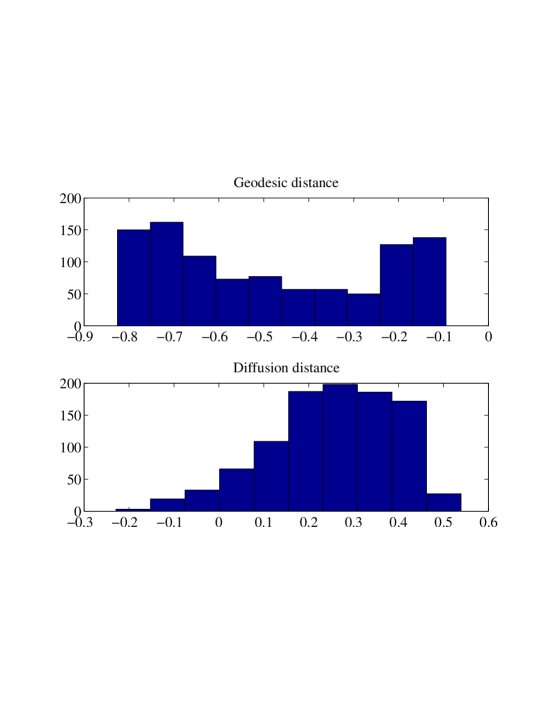
Figure 9: Sensitivity to noise. Distribution of the geodesic (top) and diffusion (bottom) distances for a noisy spiral. Each histogram has been rescaled so as to show the relative change from the noiseless case.

Figure 10: Two realizations of a noisy spiral. The solid line represents the shortest path between two reference points $A$ and $B$ in a graph constructed on the data.

Example 5

(Consistency) For a distribution not supported exactly on a manifold, the problem with shortcuts gets worse as the sample size increases. This is illustrated by our next experiment where the noise level $\beta=0.09$ and the neighborhood size $\tau=0.1$ are fixed, and the sample size $n=600,2000$ and $4000$. Figure 11 shows that for a small enough sample size, the graph estimates are close to the theoretical value $d_{\mathcal{M}}=3.46$. For intermediate sample sizes, we have a range of estimates between the Euclidean distance $\|x_{A}-x_{B}\|=0.6$ and $d_{\mathcal{M}}$. As $n$ increases, shortcuts are more likely to occur, with the graph distance eventually converging to the Euclidean distance in the ambient space.

Figure 11: Inconsistency of the geodesic graph distance. Distribution of the geodesic distance for (top to bottom) sample sizes $n=600,2000$ and $4000$. The dashed vertical lines indicate the Euclidean distance in the ambient space and the geodesic distance of the ideal manifold.

4.3 Density Sensitive Metrics

In certain machine learning methods, such as semisupervised learning, it is useful to define a density sensitive distance for which $x$ and $y$ are close just when there is a high density path connecting $x$ and $y$. This is precisely what diffusion distances do. Another such metric is (Bousquet et al., 2003)

$$d(x,y)=\inf_{q}\int_{x}^{y}\frac{ds}{p(q(s))}$$

where the infimum is over all smooth paths (parameterized by path length) connecting $x$ and $y$. The two metrics have similar goals but $\mathbf{D}_{t}(x,y)$ is more robust and easier to estimate. Indeed, to find $d(x,y)$ one has to examine all paths connecting $x$ and $y$.

5 Estimation

Now we study the properties of $\widehat{A}_{\varepsilon,t/\varepsilon}$ as an estimator of $\mathbf{A}_{t}$. Let $\Pi_{\varepsilon,\ell}$ be the orthogonal projector onto the subspace spanned by $\psi_{\varepsilon,\ell}$ and let $\Pi_{\ell}$ be the projector onto the subspace spanned by $\psi_{\ell}$. Consider the following operators:

$A_{t}(\varepsilon,P)$	$\equiv$	$A_{\varepsilon,t/\varepsilon}$ $=$ $\sum_{\ell=0}^{\infty}\lambda_{\varepsilon,\ell}^{t/\varepsilon}\ \Pi_{\varepsilon,\ell}$,	$A_{t}(\varepsilon,q,P)$	$=$	$\sum_{\ell=0}^{q}\lambda_{\varepsilon,\ell}^{t/\varepsilon}\ \Pi_{\varepsilon,\ell}$,
$A_{t}(\varepsilon,q,\widehat{P}_{n})$	$=$	$\sum_{\ell=0}^{q}\widehat{\lambda}_{\varepsilon,\ell}^{t/\varepsilon}\widehat{\Pi}_{\varepsilon,\ell}$,	$\mathbf{A}_{t}$	$=$	$\sum_{\ell\geq 0}e^{-\nu_{\ell}^{2}t}\ \Pi_{\ell}$,

where $\psi_{\varepsilon,\ell}$ and $\lambda_{\varepsilon,\ell}$ denote the eigenfunctions and eigenvalues of $A_{\varepsilon}$, and $\widehat{\psi}_{\varepsilon,\ell}$ and $\widehat{\lambda}_{\varepsilon,\ell}$ are the eigenfunctions and eigenvalues of the data-based operator $\widehat{A}_{\varepsilon}$. Two estimators of $\mathbf{A}_{t}$ are the truncated estimator $A_{t}(\varepsilon,q,\widehat{P}_{n})$ and the non-truncated estimator $A_{t}(\varepsilon,\widehat{P}_{n})\equiv e^{t(\widehat{A}_{\varepsilon}-I)/\varepsilon}$. In practice, truncation is important since it corresponds to choosing a dimension for the reparameterized data.

5.1 Estimating the Diffusion Operator $\mathbf{A}_{t}$

Given data with a sample size $n$, we estimate $\mathbf{A}_{t}$ using a finite number $q$ of eigenfunctions and a kernel bandwidth $\varepsilon>0$. We define the loss function as

$$L_{n}(\varepsilon,q,t)=\|\mathbf{A}_{t}-A_{t}(\varepsilon,q,\widehat{P}_{n})\|$$ (30)

where $\|B\|=\sup_{f\in{\cal F}}\|Bf\|_{2}/\|f\|_{2}$ and $\|f\|_{2}=\sqrt{\int_{\mathcal{X}}f^{2}(x)dP(x)}$ where ${\cal F}$ is the set of uniformly bounded, three times differentiable functions with uniformly bounded derivatives whose gradients vanish at the boundary. By decomposing $L_{n}$ into a bias-like and variance-like term (Figure 12), we derive the following result for the estimate based on truncation. Define

$$\rho(t)=\sum_{\ell=1}^{\infty}e^{-\nu_{\ell}^{2}t}.$$ (31)

Theorem 1

Suppose that $P$ has compact support, and has bounded density $p$ such that $\inf_{x}p(x)>0$ and $\sup_{x}p(x)<\infty$. Let $\varepsilon_{n}\to 0$ and $n\varepsilon_{n}^{d/2}/\log(1/\varepsilon_{n})\to\infty$. Then

$$L_{n}(\varepsilon_{n},q,t)=\rho(t)\left(O_{P}\left(\sqrt{\frac{\log(1/\varepsilon_{n})}{n\varepsilon_{n}^{(d+4)/2}}}\right)+O(\varepsilon_{n})\right)\ +\ O(1)\sum_{q+1}^{\infty}e^{-\nu_{\ell}^{2}t}.$$ (32)

The optimal choice of $\varepsilon_{n}$ is $\varepsilon_{n}\asymp(\log n/n)^{2/(d+8)}$ in which case

$$L_{n}(\varepsilon_{n},q,t)=\rho(t)\times O_{P}\left(\frac{\log n}{n}\right)^{2/(d+8)}+O(1)\sum_{q+1}^{\infty}e^{-\nu_{\ell}^{2}t}.$$ (33)

We also have the following result which does not use truncation.

Theorem 2

Define

$$A_{t}(\varepsilon,\widehat{P}_{n})=e^{t(\widehat{A}_{\varepsilon_{n}}-I)/\varepsilon_{n}}.$$

Then,

$$\|\mathbf{A}_{t}-A_{t}(\varepsilon_{n},\widehat{P}_{n})\|=\left(O_{P}\left(\sqrt{\frac{\log(1/\varepsilon_{n})}{n\varepsilon_{n}^{(d+4)/2}}}\right)+O(\varepsilon_{n})\right)\times\rho(t)$$ (34)

The optimal $\varepsilon_{n}$ is $\varepsilon_{n}\asymp(\log n/n)^{2/(d+8)}$. With this choice,

$$\|\mathbf{A}_{t}-A_{t}(\varepsilon,\widehat{P}_{n})\|=O_{P}\left(\frac{\log n}{n}\right)^{2/(d+8)}\times\rho(t).$$

Let us now make some remarks on the interpretation of these reults.

1. The terms $O(\varepsilon_{n})$ and $\sum_{q+1}^{\infty}e^{-\nu_{\ell}^{2}t}$ correspond to bias. The term $O_{P}\left(\sqrt{\frac{\log(1/\varepsilon_{n})}{n\varepsilon_{n}^{(d+4)/2}}}\right)$ corresponds to the square root of the variance.

2. The rate $n^{-2/(d+8)}$ is slow. Indeed, the variance term $1/(n\varepsilon_{n}^{(d+4)/2})$ is the usual rate for estimating the second derivative of a regression function which is a notoriously difficult problem. This suggests that estimating $\mathbf{A}_{t}$ accurately is quite difficult.

3. We also have that

   $$\|G_{\varepsilon}-\mathbf{G}\|=O_{P}\left(\sqrt{\frac{\log(1/\varepsilon_{n})}{n\varepsilon_{n}^{(d+4)/2}}}\right)+O(\varepsilon)$$

   and the first term is slower than the rate $1/\sqrt{n\varepsilon_{n}^{(d+2)/2}}$ in Giné and Koltchinskii (2006) and Singer (2006). This is because they assume a uniform distribution. The slower rate comes from the term $p_{\varepsilon}(x)-\widehat{p}_{\varepsilon}(x)$ which cannot be ignored when $p$ is unknown.

4. If the distribution is supported on a manifold of dimension $r<d$ then $\varepsilon^{(d+4)/2}$ becomes $\varepsilon^{(r+4)/2}$. In between full support and manifold support, one can create distributions that are concentrated near manifolds. That is, one first draws $X_{i}$ from a distribution supported on a lower dimensional manifold, then adds noise to $X_{i}$. This corresponds to full support again unless one lets the variance of the noise decrease with $n$. In that case, the exponent of $\varepsilon$ can be between $r$ and $d$.

5. Combining the above results with the result from Zwald and Blanchard (2006), we have that

   $$\|\psi_{\ell}-\widehat{\psi}_{\varepsilon_{n},\ell}\|=\left(O_{P}\left(\sqrt{\frac{\log(1/\varepsilon_{n})}{n\varepsilon_{n}^{(d+4)/2}}}\right)+O(\varepsilon_{n})\right)\times\frac{1}{\min_{0\leq j\leq\ell}(\nu_{j}^{2}-\nu_{j-1}^{2})}.$$

6. The function $\rho(t)$ is decreasing in $t$. Hence for large $t$, the rate of convergence can be arbitrarily fast, even for large $d$. In particular, for $t\geq\rho^{-1}(n^{-(d+4)/(2(d+8))})$ the loss has the parametric rate $O_{P}(\sqrt{\log n/n})$.

7. An estimate of the diffusion distance is

   $$\widehat{D}_{t}^{2}(x,y)=\sum_{\ell=0}^{\infty}\widehat{\lambda}_{\varepsilon,\ell}^{2t/\varepsilon}(\widehat{\psi}_{\varepsilon,\ell}(x)-\widehat{\psi}_{\varepsilon,\ell}(y))^{2}.$$

   The approximation properties are similar to those of $\widehat{A}_{t}$.

8. The dimension reduction parameter $q$ should be chosen as small as possible while keeping the last term in (32) no bigger than the first term. This is illustrated below.

Example 6

Suppose that $\nu_{\ell}=\ell^{\beta}$ for some $\beta>1/2$. Then

$$L_{n}(\varepsilon_{n},q,t) = \frac{C_{1}}{t^{1/(2\beta)}}O_{P}\left(\frac{\log n}{n^{2/(d+8)}}\right)+C_{2}e^{-tq^{2\beta}}.$$

The smallest $q_{n}$ such that the last term in (32) does not dominate is

$$q_{n}\asymp\left(\frac{\frac{1}{2\beta}\log t+\frac{2}{d+8}\log n}{t}\right)^{1/(2\beta)}$$

and we get

$$L_{n}(\varepsilon_{n},q,t)=O_{P}\left(\frac{1}{t^{1/(2\beta)}}\frac{\log n}{n^{2/(d+8)}}\right).$$

Figure 12: Decomposition of the loss into bias and variance.

5.2 Nodal Domains and Low Noise

An eigenfunction $\psi_{\ell}$ partitions the sample space into regions where $\psi_{\ell}$ has constant sign. This partition is called the nodal domain of $\psi_{\ell}$. In some sense, the nodal domain represents the basic structural information in the eigenfuction. In many applications, such as spectral clustering, it is sufficient to estimate the nodal domain rather than $\psi_{\ell}$. We will show that fast rates are sometimes available for estimating the nodal domain even when the eigenfunctions are hard to estimate. This explains why spectral methods can be very successful despite the slow rates of convergence that we and others have obtained.

Formally, the nodal domain of $\psi_{\ell}$ is $N_{\ell}=\{C_{1},\ldots,C_{k}\}$ where the sets $C_{1},\ldots,C_{k}$ partition the sample space and the sign of $\psi_{\ell}$ is constant over each partition element $C_{j}$. Thus, estimating the nodal domain corresponds to estimating $H_{\ell}(x)={\rm sign}(\psi_{\ell}(x))$.

Recently, in the literature on classification, there has been a surge of research on the so-called “low noise” case. If the data have a low probability of being close to the decision boundary, then very fast rates of convergence are possible even in high dimensions. This theory explains the success of classification techniques in high dimensional problems. In this section we show that a similar phenomema applies to spectral smoothing when estimating the nodal domain.

Inspired by the definition of low noise in Mammen and Tsybakov (1999), Audibert and Tsybakov (2007), and Kohler and Krzyzak (2007), we say that $P$ has noise exponent $\alpha$ if there exists $C>0$ such that

$$\mathbb{P}(0<|\psi_{1}(X)|\leq\delta)\leq C\delta^{\alpha}.$$ (35)

We are focusing here on $\psi_{1}$ although extensions to other eigenfunctions are immediate. Figure 13 shows 4 distributions. Each is a mixture of two Gaussians. The first column of plots shows the densities of these 4 distributions. The second column shows $\psi_{1}$. The third column shows $\mathbb{P}(0<|\psi_{1}(X)|\leq\delta)$. Generally, as clusters become well separated, $\psi_{1}$ behaves like a step function and $\mathbb{P}(0<|\psi_{1}(X)|\leq\delta)$ puts less and less mass near 0 which corresponds to $\alpha$ being large.

Figure 13: Each row corresponds to a mixture of two Gaussians. The first column of plots shows the densities of these distributions. The second column shows $\psi_{1}$. The third column shows $\mathbb{P}(0<|\psi_{1}(X)|\leq\delta)$ as a function of $\delta$.

Theorem 3

Let $H(x)={\rm sign}(\psi_{1}(x))$ and $\widehat{H}(x)={\rm sign}(\widehat{\psi}_{1}(x))$. Suppose that (35) holds. Set $\varepsilon_{n}=n^{-2/(4\alpha+d+8)}$. Then,

$$\mathbb{P}(H(X)\neq\widehat{H}(X))\leq n^{-\frac{2\alpha}{4\alpha+8+d}}$$ (36)

where $X\sim P$.

Note that, as $\alpha\to\infty$ the rate tends to the parametric rate $n^{-1/2}$.

5.3 Choosing a Bandwidth

The theory we have developed gives insight into the behavior of the methods. But we are still left with the need for a practical method for choosing $\varepsilon$. Given the similarity with kernel smoothing, it is natural to use methods from density estimation to choose $\varepsilon$. In density estimation it is common to use the loss function $\int(p(x)-\widehat{p}_{\varepsilon}(x))^{2}dx$ which is equivalent, up to a constant, to

$${\cal L}(\varepsilon)=\int\widehat{p}_{\varepsilon}^{2}(x)dx-2\int\widehat{p}_{\varepsilon}(x)p(x)dx.$$

A common method to approximate this loss is the cross-validation score

$$\widehat{\cal L}(\varepsilon)=\int\widehat{p}_{\varepsilon}^{2}(x)dx-\frac{2}{n}\sum_{i=1}^{n}\widehat{p}_{\varepsilon,i}(X_{i})$$

where $\widehat{p}_{\varepsilon,i}$ is the same as $\widehat{p}_{\varepsilon}$ except that $X_{i}$ is omitted. It is well-known that $\widehat{\cal L}(\varepsilon)$ is a nearly unbiased estimate of ${\cal L}(\varepsilon)$. One then chooses $\widetilde{\varepsilon}_{n}$ to minimize $\widehat{\cal L}(\varepsilon)$.

The optimal $\varepsilon_{n}^{*}$ from our earlier result is (up to log factors) $O(n^{-2/(d+8)})$ but the optimal bandwidth $\varepsilon_{n}^{0}$ for minimizing ${\cal L}$ is $O(n^{-2/(d+4)})$. Hence, $\varepsilon_{n}^{*}/\varepsilon_{n}^{0}\asymp n^{8/((d+4)(d+8))}$. This suggests that density cross-validation is not appropriate for our purposes.

Indeed, there appears to be no unbiased risk estimator for this problem. In fact, estimating the risk is difficult in most problems that are not prediction problems. As usual in nonparametric inference, the problem is that estimating bias is harder than the original estimation problem. Instead, we take a more modest view of simply trying to find the smallest $\varepsilon$ such that the resulting variability is tolerable. In other words, we choose the smallest $\varepsilon$ that leads to stable estimates of the eigenstructure (similar to the approach for choosing the number of clusters in Lange et al. (2004)). There are several ways to do this as we now explain.

Eigen-Stability. Define $\overline{\psi}_{\varepsilon,\ell}(x)=\mathbb{E}(\widehat{\psi}_{\varepsilon,\ell}(x))$. Although $\overline{\psi}_{\varepsilon,\ell}\neq\psi_{\ell}$, they do have a similar shape. We propose to choose $\varepsilon$ by finding the smallest $\varepsilon$ for which $\overline{\psi}_{\varepsilon,\ell}$ can be estimated with a tolerable variance. To this end we define

$${\rm SNR}(\varepsilon)=\sqrt{\frac{||\overline{\psi}_{\varepsilon,\ell}||_{2}^{2}}{\mathbb{E}||\widehat{\psi}_{\ell}-\overline{\psi}_{\varepsilon,\ell}||_{2}^{2}}}$$ (37)

which we will refer to as the signal-to-noise ratio. When $\varepsilon$ is small, the denominator will dominate and ${\rm SNR}(\varepsilon)\approx 0$. Conversely, when $\varepsilon$ is large, the denominator tends to 0 so that ${\rm SNR}(\varepsilon)$ gets very large. We want to find $\varepsilon_{0}$ such that

$$\varepsilon_{0}=\inf\Biggl{\{}\varepsilon:\ {\rm SNR}(\varepsilon)\geq K_{n}\Biggr{\}}$$

for some $K_{n}\geq 1$.

We can estimate ${\rm SNR}$ as follows. We compute $B$ bootstrap replications

$$\widehat{\psi}_{\varepsilon,\ell}^{(1)},\ldots,\widehat{\psi}_{\varepsilon,\ell}^{(B)}.$$

We then take

$$\widehat{\rm SNR}(\varepsilon)=\sqrt{\frac{\left(||\overline{\psi}_{\varepsilon,\ell}^{*}||^{2}_{2}-\xi^{2}\right)_{+}}{\xi^{2}}}$$ (38)

where $c_{+}=\max\{c,0\}$,

$$\xi^{2}=\frac{1}{B}\sum_{b=1}^{B}||\widehat{\psi}_{\varepsilon,\ell}^{(b)}-\overline{\psi}_{\varepsilon,\ell}^{*}||^{2}_{2}$$

and $\overline{\psi}_{\varepsilon,\ell}^{*}=B^{-1}\sum_{b=1}^{B}\widehat{\psi}_{\varepsilon,\ell}^{(b)}$. Note that we subtract $\xi^{2}$ from the numerator to make the numerator approximately an unbiased estimator of $||\overline{\psi}_{\varepsilon,\ell}||^{2}$. Then we use

$$\widehat{\varepsilon}=\min\bigl{\{}\varepsilon:\ \widehat{\rm SNR}(\varepsilon)\geq K_{n}\bigr{\}}.$$

We illustrate the method in Section 6. For $K_{n}=Cn^{2/(d+8)}$, where $C$ is a constant, the optimal $\varepsilon$ is $O(n^{-2/(d+8)})$. To see this, write

$$\widehat{\psi}_{\varepsilon,\ell}(x)=\psi_{\ell}(x)+b(x)+\xi(x)$$

where $b(x)$ denotes the bias and $\xi(x)=\widehat{\psi}_{\varepsilon,\ell}(x)-\psi_{\ell}(x)-b(x)$ is the random component. Then

$${\rm SNR}^{2}(\varepsilon)=\frac{||\psi_{\ell}(x)+b(x)||^{2}}{\mathbb{E}||\xi||^{2}}=\frac{O(1)}{O_{P}\left(\frac{1}{n\varepsilon^{(d+4)/2}}\right)}.$$

Setting this equal to $K_{n}^{2}$ yields $\varepsilon_{0}=O(n^{-2/(d+8)})$.

The same bootstrap idea can be applied to estimating the nodal domain. In this case we define

$$\widehat{\rm SNR}(\varepsilon)=\sqrt{\frac{\left(||\overline{H}_{\varepsilon,\ell}^{*}||^{2}_{2}-\xi^{2}\right)_{+}}{\xi^{2}}}$$ (39)

where

$$\xi^{2}=\frac{1}{B}\sum_{b=1}^{B}||\widehat{H}_{\varepsilon,\ell}^{(b)}-\overline{H}_{\varepsilon,\ell}^{*}||^{2}_{2}$$

and $\overline{H}_{\varepsilon,\ell}^{*}=B^{-1}\sum_{b=1}^{B}\widehat{H}_{\varepsilon,\ell}^{(b)}$.

Neighborhood Size Stability. Another way to control the variability is to ensure that the number of points involved in the local averages does not get too small. For a given $\varepsilon$ let $N=\{N_{1},\ldots,N_{n}\}$ where $N_{i}=\#\{X_{j}:\ \|X_{i}-X_{j}\|\leq\sqrt{2\epsilon}\}$. One can informally examine the histogram of $N$ for various $\varepsilon$. A rule for selecting $\varepsilon$ is

$$\widehat{\varepsilon}=\min\bigl{\{}\varepsilon:\ {\rm median}\{N_{1},\ldots,N_{n}\}\geq k\bigr{\}}.$$

We illustrate the method in Section 6.

An alternative, suggested by von Luxburg (2007), is to choose the smallest $\varepsilon$ that makes the resulting graph well-connected. This leads to $\varepsilon=O((\log n/n)^{1/d})$. More specifically, von Luxburg (2007) suggests to “… choose $\varepsilon$ as the length of the longest edge in a minimal spanning tree of the fully connected graph on the data points.”

6 Examples

6.1 Two Gaussians

Let

$$p(x)=\frac{1}{2}\phi(x;-2,1)+\frac{1}{2}\phi(x;2,1)$$

where $\phi(x;\mu,\sigma)$ denotes a Normal density with mean $\mu$ and variance $\sigma^{2}$. Figure 14 shows the error $\|\psi_{1}-\widehat{\psi}_{\varepsilon,1}\|$ as a function of $\varepsilon$ for a sample of size $n=1000$. The results are averaged over approximately  $200$ independent draws. A minimal error occurs for a range of different values of $\varepsilon$ between $0.03$ and $0.1$. The variance dominates the error in the small $\varepsilon$ region ($\varepsilon<0.03$) , while the bias dominates in the large $\varepsilon$ region ($\varepsilon>0.1$). These results are consistent with Figure 15, which shows the estimated mean and variance of the first eigenvector $\widehat{\psi}_{\varepsilon,1}$ for a few selected values of $\varepsilon$ ($\varepsilon=0.02,0.03,0.1,1$), marked with blue circles in Figure 14. Figures 16-18 show similar results for the second, third and fourth eigenvectors $\psi_{2},\psi_{3},\psi_{4}$. Note that even in cases where the error in the estimates of the eigenvectors is large, the variance around the cross-over points (where the eigenvectors switch signs) can be small.

Figure 19 (left) shows a histogram of $N_{i}=\#\{X_{j}:\ \|X_{i}-X_{j}\|\leq\sqrt{2\varepsilon}\}$ for $\varepsilon=0.02,0.03,0.1,1$ and $n=1000$. All results are averaged over $500$ independent simulations. The vertical dashed lines indicate the median values. For this particular example, we know that the error is small when $\varepsilon$ is between $0.03$ and $0.1$. This corresponds to ${\rm median}\{N_{1},\ldots,N_{n}\}$ being around $100$. Figure 19 (right) shows a histogram of the distance to the $k$-nearest neighbor for $k=100$. The median value $0.32$ (see vertical dashed line) roughly corresponds to the tuning parameter $\varepsilon=0.32^{2}/2=0.05$.

Figure 14: The error $\|\psi_{1}-\widehat{\psi}_{\varepsilon,1}\|$ in the estimate of the first eigenvector as a function of $\varepsilon$. For each $\varepsilon$ (red dots), an average is taken over approximately $200$ independent simulations with $n=1000$ points from a mixture distribution with two Gaussians. Figure 15 shows the estimated mean and variance of $\widehat{\psi}_{\varepsilon,1}$ for $\varepsilon=0.02,0.03,0.1,1$ (blue circles)

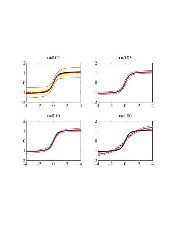
Figure 15: The first eigenvector $\widehat{\psi}_{\varepsilon,1}$ for $\varepsilon=0.02,0.03,0.1,1$ and $n=1000$. The red dashed curves with shaded regions indicate the mean value $\pm$ two standard deviations for approximately $300$ independent simulations. The black solid curves show ${\psi}_{\varepsilon,1}$ as $\varepsilon\rightarrow 0$.

Figure 16: The second eigenvector $\widehat{\psi}_{\varepsilon,2}$ for $\varepsilon=0.02,0.03,0.1,1$ and $n=1000$. The red dashed curves with shaded regions indicate the mean value $\pm$ two standard deviations for approximately $300$ independent simulations. The black solid curves show ${\psi}_{\varepsilon,2}$ as $\varepsilon\rightarrow 0$.

Figure 17: The third eigenvector $\widehat{\psi}_{\varepsilon,3}$ for $\varepsilon=0.02,0.03,0.1,1$ and $n=1000$. The red dashed curves with shaded regions indicate the mean value $\pm$ two standard deviations for approximately $300$ independent simulations. The black solid curves show ${\psi}_{\varepsilon,3}$ as $\varepsilon\rightarrow 0$.

Figure 18: The fourth eigenvector $\widehat{\psi}_{\varepsilon,4}$ for $\varepsilon=0.02,0.03,0.1,1$ and $n=1000$. The red dashed curves with shaded regions indicate the mean value $\pm$ two standard deviations for approximately $300$ independent simulations. The black solid curves show ${\psi}_{\varepsilon,4}$ as $\varepsilon\rightarrow 0$.

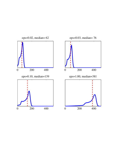
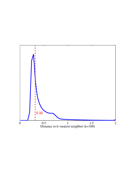
Figure 19: Left: Histogram of $N_{i}=\#\{X_{j}:\ \|X_{i}-X_{j}\|\leq\sqrt{2\epsilon}\}$ for $\varepsilon=0.02,0.03,0.1,1$ and $n=1000$. The vertical dashed lines indicate the median values. Right: Histogram of the distance to the $k$-nearest neighbor for $k=100$. The median value $0.32$ (vertical dashed line) roughly corresponds to $\varepsilon=0.32^{2}/2=0.05$. All results are averaged over $500$ independent simulations.

Choosing the Bandwidth Using SNR. Figure 20 (line with circles) shows the signal-to-noise ratio for $\psi_{1}$ with $n=1000$, estimated by simulation. For each simulation, we also computed the bootstrap estimate of SNR and averaged this over the simulations. The result is the line with triangles. The dashed lines in Figure 21 represent bootstrap estimates of SNR for three typical data sets. The resulting $\widehat{\psi}_{\widehat{\varepsilon},1}$ using $SNR=5$ are shown to the right. For all three data sets, the bootstrap estimates of $\psi_{1}$ (dashed lines) almost overlap the true eigenvector (solid line).

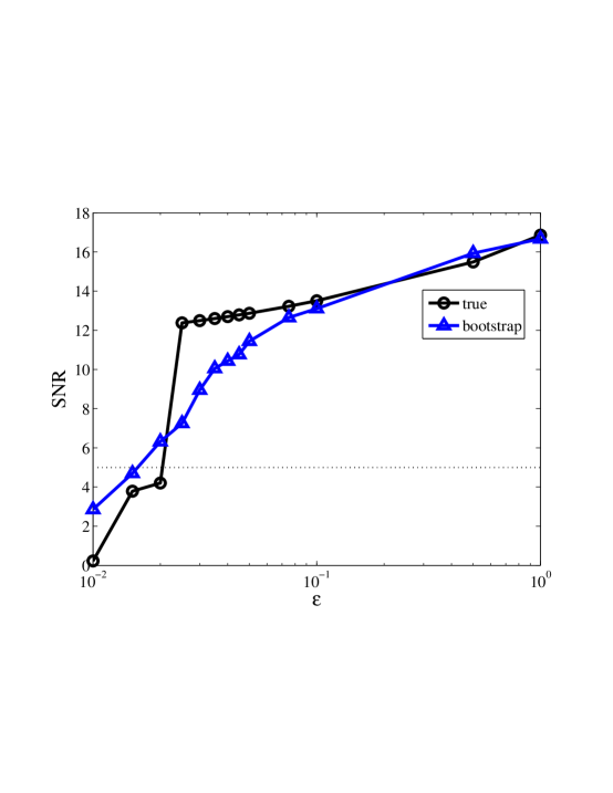
Figure 20: True signal-to-noise ratio estimated by simulation (rings) and mean of the bootstrap estimated signal-to-noise ratio (triangles) as a function of $\varepsilon$.

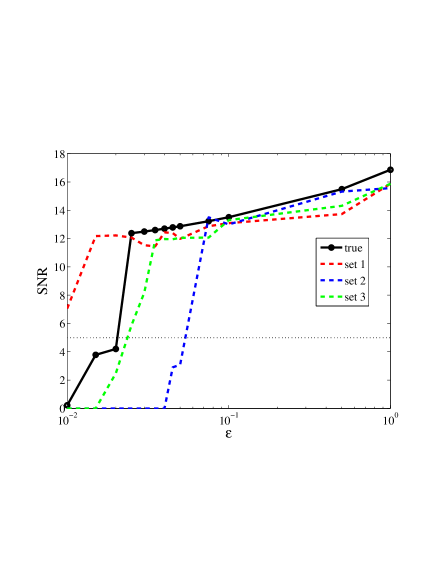
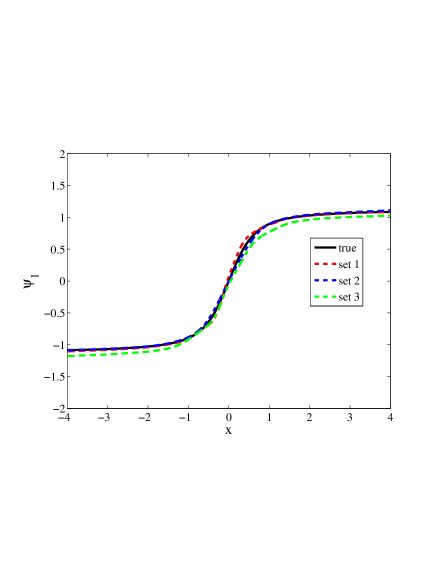
Figure 21: Left: Signal-to-noise ratio, as a function of $\varepsilon$, estimated by simulation (solid black line), and by the bootstrap for three different data sets (dashed lines). Right: $\psi_{1}$ (solid black line) and resulting bootstrap estimates of $\psi_{1}$ using SNR = 5 (dashed lines).

Estimating the Nodal Domain. Now consider estimating $H_{\ell}(x)={\rm sign}(\psi_{\ell}(x))$. Figure 22 shows the nodal domain error for $H_{\ell}$ when $\ell=1,2,3,4$, estimated by simulation. We see that the error is relatively small and stable over $\varepsilon$. As predicted by our results, large $\varepsilon$ can lead to very low error. We can use the instability measure $\Xi(\varepsilon,\ell)=\mathbb{P}(\widehat{H}_{\ell}(X)\neq H_{\ell}(X))$, where $\widehat{H}_{\ell}(x)={\rm sign}(\widehat{\psi}_{\varepsilon,\ell}(x))$, to choose $\varepsilon$ and $q$. For example, find the smallest $\varepsilon$ and the largest number $q$ of eigenvectors such that $\widehat{\Xi}(\varepsilon,\ell)\leq\alpha$ for all $\ell\leq q$. (In this case, $\alpha=0.2$ approximately corresponds to $\varepsilon=0.075$ and $q=4$.) We should caution the reader, however, that stability-based ideas have drawbacks. In clustering, for example, Ben-David et al. (2006) showed that choosing the number of clusters based on stability can lead to poor clusters.

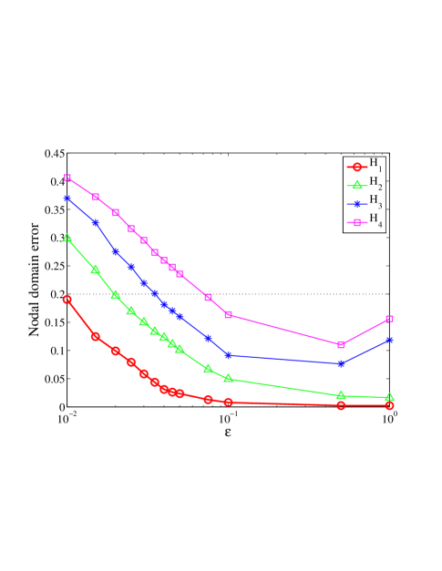
Figure 22: The nodal domain error $\mathbb{P}(\widehat{H}_{\ell}(X)\neq H_{\ell}(X))$ as a function of $\varepsilon$ for $\ell=1,2,3,4$.

6.2 Words

The last example is an application of SCA to text data mining. The example shows how one can measure the semantic association of words using diffusion distances, and how one can organize and form representative “meta-words” by eigenanalysis and quantization of the diffusion operator.

The data consist of $p=1161$ Science News articles. To encode the text, we extract $n=1004$ words (see Lafon and Lee (2006) for details) and form a document-word information matrix. The mutual information between document $x$ and word $y$ is defined as

$$I_{x,\,y}=\log\left(\frac{f_{x,\,y}}{\sum_{\xi}f_{\xi,\,y}\sum_{\eta}f_{\xi,\eta}}\right)\ ,$$

where $f_{x,y}=c_{x,y}/n$, and $c_{x,y}$ is the number of times word $y$ appears in document $x$. Let

$$e_{y}=[I_{1,\,y},I_{2,\,y},\ldots I_{p,\,y}]\ .$$

be a p-dimensional feature vector for word $y$.

Our goal is to reduce both the dimension $p$ and the number of variables $n$, while preserving the main connectivity structure of the data. In addition, we seek a parameterization of the words that reflect how similar they are in meaning. Diffusion maps and diffusion coarse-graining (quantization) offer a natural framework for achieving these objectives.

Define the weight matrix $\mathbb{K}(i,j)=\exp\left(-\frac{\|e_{i}-e_{j}\|^{2}}{4\varepsilon}\right)$ for a graph with $n$ nodes. Let $\mathbb{A}_{\varepsilon,m}$ be the corresponding $m$-step transition matrix with eigenvalues $\lambda_{\ell}^{m}$ and eigenvectors $\psi_{\ell}$. Using the bootstrap, we estimate the SNR of $\psi_{1}$ as a function of $\varepsilon$ (Figure 23, left). A SNR cut-off at 2, gives the bandwidth $\varepsilon=150$. Figure 23, right, shows the spectral fall-off for this choice of $\varepsilon$. For $m=3$ and $q=12$, we have that $(\lambda_{q}/\lambda_{1})^{m}<0.1$, i.e we can obtain a dimensionality reduction of a factor of about $1/100$ by the eigenmap $e_{y}\in\mathbb{R}^{p}\ \mapsto(\lambda_{1}^{m}\psi_{1}(y),\lambda_{2}^{m}\psi_{2}(y),\ldots,\lambda_{q}^{m}\psi_{q}(y))\in\mathbb{R}^{q}$ without losing much accuracy. Finally, to reduce the number of variables $n$, we form a quantized matrix $\widetilde{\mathbb{A}}_{\varepsilon,m}$ for a coarse-grained random walk on a graph with $k<n$ nodes. It can be shown (Lafon and Lee, 2006), that the spectral properties of $\mathbb{A}_{\varepsilon,m}$ and $\widetilde{\mathbb{A}}_{\varepsilon,m}$ are similar when the coarse-graining (quantization) corresponds to $k$-means clustering in diffusion space.

Figure 24 shows the first two diffusion coordinates of the cluster centers (the “meta-words”) for $k=100$. These representative words have roughly been rearranged according to their semantics and can be used as conceptual indices for document representation and text retrieval. Starting to the left, moving counter-clockwise, we here have words that express concepts in medicine, biology, earth sciences, physics, astronomy, computer science and social sciences. Table 2 gives examples of words in a cluster and the corresponding word centers.

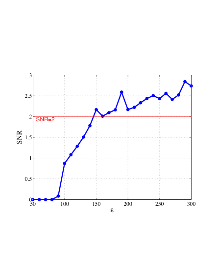
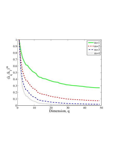
Figure 23: Left: Estimated SNR of $\psi_{1}$ as a function of $\varepsilon$. Right: Decay of the eigenvalues of $\mathbb{A}_{\varepsilon,m}$ for $\varepsilon=150$ and $m=1,2,3,4$.

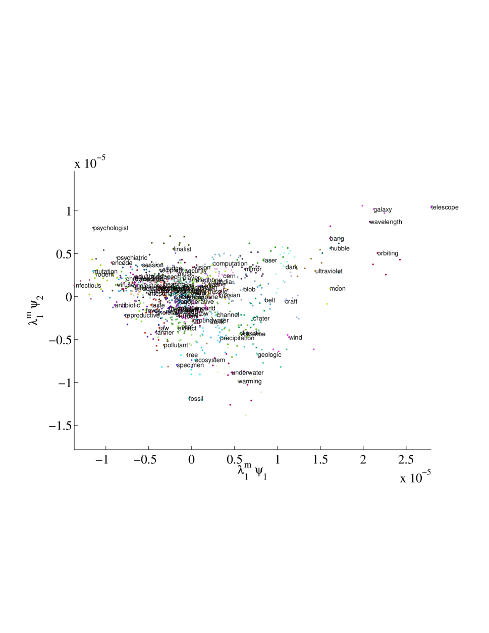
Figure 24: Parameterization and grouping of words using diffusion mapping. The text labels the representative word centers (meta-words) in each group. Note that the words are roughly arranged according to their semantic meaning.

Table 2: Examples of word groupings

Word center	Remaining words in group
virus	aids, allergy, hiv, vaccine, viral
reproductive	fruit, male, offspring, reproductive, sex, sperm
vitamin	calory, drinking, fda, sugar, supplement, vegetable
fever	epidemic, lethal, outbreak, toxin
ecosystem	ecologist, fish, forest, marine, river, soil, tropical
warming	climate, el, nino, forecast, pacific, rain, weather, winter
geologic	beneath, crust, depth, earthquake, plate, seismic, trapped, volcanic
laser	atomic, beam, crystal, nanometer, optical, photon, pulse, quantum, semiconductor
hubble	dust, gravitational, gravity, infrared
galaxy	cosmic, universe
finalist	award, competition, intel, prize, scholarship, student, talent, winner

7 Discussion

Spectral methods are rapidly gaining popularity. Their ability to reveal nonlinear structure makes them ideal for complex, high-dimensional problems. We have attempted to provide insight into these techniques by identifying the population quantities that are being estimated and studying their large sample properties.

Our analysis shows that spectral kernel methods in most cases have a convergence rate similar to classical non-parametric smoothing. Laplacian-based kernel methods, for example, use the same smoothing operators as in traditional nonparametric regression. The end goal however is not smoothing, but data parameterization and structure definition of data. Spectral methods exploit the fact that the eigenvectors of local smoothing operators provide information on the underlying geometry and connectivity of the data.

We close by briefly mention how SCA and diffusion maps also can be used in clustering, density estimation and regression. The full details of these applications will be reported in separate papers.

7.1 Clustering

One approach to clustering is spectral clustering. The idea is to reparameterize the data using the first few nontrivial eigenvectors $\psi_{1},\ldots,\psi_{m}$ and then apply a standard clustering algorithm such as $k$-means clustering. This can be quite effective for finding non-spherical clusters.

Diffusion distances can also be used for this purpose. Recall that ordinary $k$-means clustering seeks to find points $C=\{c_{1},\ldots,c_{k}\}$ to minimize the empirical distortion

$$\widehat{\Delta}(C)=\frac{1}{n}\sum_{i=1}^{n}\|X_{i}-Q_{C}(X_{i})\|^{2}$$

where $Q_{C}$ is the quantization map that takes $X_{i}$ to the closest $c_{j}\in C$. The empirical distortion estimates the population distortion

$$\Delta(C)=\mathbb{E}\|X-Q_{C}(X)\|^{2}.$$

By using $k$-means in diffusion map coordinates we instead minimize

$$\Delta(C)=\mathbb{E}D_{t}(X,Q_{t}(X))$$

where $Q_{t}(x)={\rm argmin}_{c\in C}D_{t}(x,c)$. The details are in Lee and Wasserman (2008).

7.2 Density Estimation

If $Q$ is a quanization map then the quantized density estimator (Meinicke and Ritter, 2002) is

$$\widehat{p}(x)=\frac{1}{n}\sum_{i=1}^{n}\frac{1}{h^{d}}K_{h}(\|x-Q(X_{i})\|).$$

For highly clustered data, the quantized density estimator can have smaller mean squared error than the usual kernel density estimator. Similarly, we can define the quantized diffusion density estimator as

$$\widehat{p}(x)=\frac{1}{n}\sum_{i=1}^{n}\frac{1}{h^{d}}K(\widehat{D}_{t}(x,X_{i}))$$

which can potentially have small mean squared error for appropriately chosen $t$. See Buchman et al. (2008) for an application to density estimation of hurricane tracks in the Atlantic Ocean.

7.3 Regression

A common method for nonparametric regression is to expand the regression function $m(x)=\mathbb{E}(Y|X=x)$ in a basis and then estimate the coefficients of the expansion from the data. Usually, the basis is chosen beforehand. The diffusion map basis provides a natural data-adaptive basis for doing nonparametric regression. We expand $m(x)=\mathbb{E}(Y|X=x)$ as $m(x)=\sum_{j}\beta_{j}\psi_{j}(x)$. Let $\widehat{m}(x)=\sum_{j=1}^{q}\widehat{\beta}_{j}\widehat{\psi}_{\varepsilon,j}(x)$ where $q$ and $\varepsilon$ are chosen by cross-validation. See Richards et al. (2009) for an application to astronomy data and spectroscopic redshift prediction.

8 Appendix

8.1 Spectral Decomposition and Euclidean Distances in Diffusion Space

In this section, we describe how a symmetric operator $\widetilde{A}$, the stochastic differential operator $A$ and its adjoint (the Markov operator) $A^{*}$ are related, and how these relations lead to different normalization schemes for the corresponding eigenvectors. (For ease of notation, we have omitted the subindex ${\varepsilon}$, since we here consider a fixed $\varepsilon>0$.) We also show that the diffusion metric corresponds to a weighted Euclidean distance in the embedding space induced by the diffusion map.

Suppose that $P$ is a probability measure with a compact support $\mathcal{X}$. Let $k:\mathcal{X}\times\mathcal{X}$ be a similarity function that is symmetric, continuous, and positivity-preserving, i.e. $k(x,y)>0$ for all $x,y\in\mathcal{X}$. For simplicity, we assume in addition that $k$ is positive semi-definite, i.e. for all bounded functions $f$ on $\mathcal{X}$, $\int_{\mathcal{X}}\int_{\mathcal{X}}k(x,y)f(x)f(y)dP(x)dP(y)\geq 0$. Consider two different normalization schemes of $k$:

$$\begin{array}[]{llll}\widetilde{a}(x,y)&=&\frac{k(x,y)}{\sqrt{\rho(x)}\sqrt{p(y)}}&\ \ \ \ \ \rm{(symmetric)}\\ a(x,y)&=&\frac{k(x,y)}{\rho(x)}&\ \ \ \ \ \rm{(stochastic)}\end{array}$$

where $\rho(x)=\int k(x,y)dP(y)$.

Define the symmetric integral operator $\widetilde{A}$ by

$$\widetilde{A}f(x)=\int_{\mathcal{X}}\widetilde{a}(x,y)f(y)dP(y).$$

Under the stated conditions, $k(x,y)$ is an $L^{2}$-kernel. It follows that $\widetilde{A}$ is a self-adjoint compact operator. The eigenvalues $\{\lambda_{\ell}\}_{\ell\geq 0}$ of $\widetilde{A}$ are real and the associated eigenfunctions $\{v_{\ell}\}_{\ell\geq 0}$ form an orthonormal basis of $L^{2}(\mathcal{X};dP)$. According to Mercer’s theorem, we have the spectral decomposition

$$\widetilde{a}(x,y)=\sum_{\ell\geq 0}\lambda_{\ell}v_{\ell}(x)v_{\ell}(y),$$ (40)

where the series on the right converges uniformly and absolutely to $\widetilde{a}(x,y)$.

Now consider the integral operator $A$ and its adjoint (the Markov operator) $A^{*}$:

$$\begin{array}[]{lll}Af(x)&=&\int_{\mathcal{X}}a(x,y)f(y)dP(y)\\ A^{*}f(x)&=&\int_{\mathcal{X}}f(y)a(y,x)dP(y),\\ \end{array}$$

where $\langle Af,g\rangle_{L^{2}(\mathcal{X};dP)}=\langle f,A^{*}g\rangle_{L^{2}(\mathcal{X};dP)}$. Let $\ s(x)=\rho(x)/\int\rho(y)dP(y)$. If $\widetilde{A}v_{\ell}=\lambda_{\ell}v_{\ell}$, then we have the corresponding eigenvalue equations

$$A\psi_{\ell}=\lambda_{\ell}\psi_{\ell},\ \ {\rm where}\ \ \psi_{\ell}(x)=v_{\ell}(x)/\sqrt{s(x)}$$ (41)

and

$$A^{*}\varphi_{\ell}=\lambda_{\ell}\varphi_{\ell},\ \ {\rm where}\ \ \varphi_{\ell}(x)=v_{\ell}(x)\sqrt{s(x)}.$$ (42)

Moreover, if $\{v_{\ell}\}_{\ell\geq 0}$ is an orthonormal basis of $L^{2}(\mathcal{X};dP)$, then the sets $\{\psi_{\ell}\}_{\ell\geq 0}$ and $\{\varphi_{\ell}\}_{\ell\geq 0}$ form orthonormal bases of the weighted $L^{2}$-spaces $L^{2}(\mathcal{X};sdP)$ and $L^{2}(\mathcal{X};dP/s)$, respectively. The operator $A$ preserves constant functions, i.e. $A1=1$. One can also show that the matrix norm $\|\widetilde{A}\|=\sup_{f\in L^{2}(\mathcal{X};dP)}\frac{\|\widetilde{A}f\|}{\|f\|}=1$. Thus, the eigenvalue $\lambda_{0}=1$ is the largest eigenvalue of the operators $A$ and $A^{*}$. The corresponding eigenvector of $A$ is $\psi_{0}=1$, and the corresponding eigenvector of $A^{*}$ is $\varphi_{0}=s$.

From Eq. 40, it follows that

$$a(x,y)=\sum_{\ell\geq 0}\lambda_{\ell}\psi_{\ell}(x)\varphi_{\ell}(y),$$

where $\|\varphi_{\ell}\|_{L^{2}(\mathcal{X};dP/s)}=\|\psi_{\ell}\|_{L^{2}(\mathcal{X};sdP)}=1$ for all $\ell\geq 0$, and $\langle\varphi_{k},\psi_{\ell}\rangle_{L^{2}(\mathcal{X};dP)}=0$ for $k\neq\ell$. More generally, if $a_{m}(x,y)$ is the kernel of the $m^{\rm th}$ iterate $A^{m}$, where $m$ is a positive integer, then

$$a_{m}(x,y)=\sum_{\ell\geq 0}\lambda_{\ell}^{m}\psi_{\ell}(x)\varphi_{\ell}(y).$$ (43)

We define a one-parametric family of diffusion distances between points $x$ and $z$ according to

$$D_{m}^{2}(x,z)\equiv\|a_{m}(x,\cdot)-a_{m}(z,\cdot)\|^{2}_{L^{2}(\mathcal{X};dP/s)},$$ (44)

where the parameter $m$ determines the scale of the analysis. The diffusion metric measures the rate of connectivity between points on a data set. It will be small if there are many paths of lengths less than or equal to $2m$ between the two points, and it will be large if the number of connections is small. One can see this clearly by expanding the expression in Eq. 44 so that

$$D_{m}^{2}(x,z)=\frac{a_{2m}(x,x)}{s(x)}+\frac{a_{2m}(z,z)}{s(z)}-\left(\frac{a_{2m}(x,z)}{s(z)}+\frac{a_{2m}(z,x)}{s(x)}\right).$$ (45)

The quantity $D_{m}^{2}(x,z)$ is small when the transition probability densities $a_{2m}(x,z)$ and $a_{2m}(z,x)$ are large.

Finally, we look for an embedding where Euclidean distances reflect the above diffusion metric. The biorthogonal decomposition in Eq. 43 can be viewed as an orthogonal expansion of the functions $a_{m}(x,\cdot)$ with respect to the orthonormal basis $\{\varphi_{\ell}\}_{\ell\geq 0}$ of $L^{2}(\mathcal{X};dP/s)$; the expansion coefficients are given by $\{\lambda_{\ell}^{m}\psi_{\ell}(x)\}_{\ell\geq 0}$. Hence,

$$D_{m}^{2}(x,z)=\sum_{\ell\geq 0}(\lambda_{\ell}^{m}\psi_{\ell}(x)-\lambda_{\ell}^{m}\psi_{\ell}(z))^{2}=\|\Psi_{m}(x)-\Psi_{m}(z)\|^{2},$$

where $\Psi_{m}:x\mapsto(\lambda_{1}^{m}\psi_{1}(x),\lambda_{2}^{m}\psi_{2}(x),\ldots)$ is the diffusion map of the data at time step $m$.

8.2 Proofs

Proof of Theorem 1. From Theorem 2 below, we have that

$$\|A_{t}(\varepsilon_{n},\widehat{P}_{n})-\mathbf{A}_{t}\|=\left(O_{P}\left(\sqrt{\frac{\log(1/\varepsilon_{n})}{n\varepsilon_{n}^{(d+4)/2}}}\right)+O(\varepsilon_{n})\right)\times\rho(t).$$

Hence,

$$\|A_{t}(\varepsilon_{n},q,\widehat{P}_{n})-\mathbf{A}_{t}\| \leq \|A_{t}(\varepsilon_{n},q,\widehat{P}_{n})-A_{t}(\varepsilon_{n},\widehat{P}_{n})\|+\|A_{t}(\varepsilon_{n},\widehat{P}_{n})-\mathbf{A}_{t}\|$$

$$= \|A_{t}(\varepsilon_{n},q,\widehat{P}_{n})-A_{t}(\varepsilon_{n},\widehat{P}_{n})\|+\left(O_{P}\left(\sqrt{\frac{\log(1/\varepsilon_{n})}{n\varepsilon_{n}^{(d+4)/2}}}\right)+O(\varepsilon_{n})\right)\times\rho(t)$$

$$= \|\sum_{q+1}^{\infty}\widehat{\lambda}_{\varepsilon_{n},\ell}^{t/\varepsilon_{n}}\widehat{\Pi}_{\varepsilon_{n},\ell}\|+\left(O_{P}\left(\sqrt{\frac{\log(1/\varepsilon_{n})}{n\varepsilon_{n}^{(d+4)/2}}}\right)+O(\varepsilon_{n})\right)\times\rho(t)$$

$$\leq \sum_{q+1}^{\infty}\widehat{\lambda}_{\varepsilon_{n},\ell}^{t/\varepsilon_{n}}+\left(O_{P}\left(\sqrt{\frac{\log(1/\varepsilon_{n})}{n\varepsilon_{n}^{(d+4)/2}}}\right)+O(\varepsilon_{n})\right)\times\rho(t).$$

Now we bound the first sum. Note that,

$$\sup_{\ell}|\widehat{\nu}_{\varepsilon_{n},\ell}^{2}-\nu_{\varepsilon_{n},\ell}^{2}|=\sup_{\ell}\frac{|\widehat{\lambda}_{\varepsilon_{n},\ell}-\lambda_{\varepsilon_{n},\ell}|}{\varepsilon_{n}}\leq\frac{\|\widehat{A}_{\varepsilon_{n}}-A_{\varepsilon_{n}}\|}{\varepsilon_{n}}=O_{P}(\gamma_{n})$$

where

$$\gamma_{n}=\sqrt{\frac{\log(1/\varepsilon_{n})}{n\varepsilon_{n}^{(d+4)/2}}}.$$

By a Taylor series expansion,

$$G_{\varepsilon_{n}}f=\mathbf{G}f+O(\varepsilon_{n})$$

uniformly for $f\in{\cal F}$. (This is the same calculation used to compute the bias in kernel regression. See also, Giné and Koltchinskii (2006) and Singer (2006)). So,

$$\sup_{\ell}|\nu_{\varepsilon_{n},\ell}^{2}-\nu_{\ell}^{2}|\leq\|G_{\varepsilon_{n}}-\mathbf{G}\|=O(\varepsilon_{n}).$$

Therefore,

$$\sum_{q+1}^{\infty}\widehat{\lambda}_{\varepsilon_{n},\ell}^{t/\varepsilon_{n}} = \sum_{q+1}^{\infty}(1-\varepsilon_{n}\widehat{\nu}_{\varepsilon_{n},\ell}^{2})^{t/\varepsilon_{n}}$$

$$= \sum_{q+1}^{\infty}\exp\left\{\frac{t}{\varepsilon_{n}}\log(1-\varepsilon_{n}\widehat{\nu}_{\varepsilon_{n},\ell}^{2})\right\}$$

$$= \sum_{q+1}^{\infty}\exp\left\{\frac{t}{\varepsilon_{n}}\log(1-\varepsilon_{n}[O_{P}(\gamma_{n})+O(\varepsilon_{n})-\nu_{\ell}^{2}])\right\}$$

$$= (1+O_{P}(\gamma_{n})+O(\varepsilon_{n}))\sum_{q+1}^{\infty}e^{-\nu_{\ell}^{2}t}.$$

In conclusion,

$$\|A_{t}(\varepsilon_{n},q,\widehat{P}_{n})-\mathbf{A}_{t}\| = \left(O_{P}\left(\sqrt{\frac{\log(1/\varepsilon_{n})}{n\varepsilon_{n}^{(d+4)/2}}}\right)+O(\varepsilon_{n})\right)\times\rho(t)$$

$$\ \ \ +\ \ \Biggl{(}1+O_{P}(\gamma_{n})+O(\varepsilon_{n})\Biggr{)}\sum_{q+1}^{\infty}e^{-\nu_{\ell}^{2}t}$$

$$\leq \rho(t)\left(O_{P}\left(\sqrt{\frac{\log(1/\varepsilon_{n})}{n\varepsilon_{n}^{(d+4)/2}}}\right)+O(\varepsilon_{n})\right)\ +\ \sum_{q+1}^{\infty}e^{-\nu_{\ell}^{2}t}.$$

Proof of Theorem 2. Recall that $A_{t}(\varepsilon_{n},\widehat{P}_{n})=e^{t(\widehat{A}_{\varepsilon_{n}}-I)/\varepsilon_{n}}$. From lemma 1, $\|A_{\varepsilon}-\widehat{A}_{\varepsilon}\|=\gamma(\varepsilon)$ where

$$\gamma(\varepsilon)=O_{P}\left(\sqrt{\frac{\log(1/\varepsilon_{n})}{n\varepsilon_{n}^{d/2}}}\right).$$

Hence,

$$\frac{\widehat{A}_{\varepsilon}-I}{\varepsilon} = \frac{\widehat{A}_{\varepsilon}-A_{\varepsilon}}{\varepsilon}+\frac{A_{\varepsilon}-I}{\varepsilon}=\frac{\gamma(\varepsilon)}{\varepsilon}+\mathbf{G}+O(\varepsilon)$$

and so

$$A_{t}(\varepsilon,\widehat{P}_{n})=\mathbf{A}_{t}e^{t(\gamma(\varepsilon)+O(\varepsilon^{2})/\varepsilon}=\mathbf{A}_{t}\Biggl{[}I+t\bigl{(}\gamma(\varepsilon)+O(\varepsilon^{2})\bigr{)}/\varepsilon+o\bigl{(}t(\gamma(\varepsilon)+O(\varepsilon))\bigr{)}/\varepsilon\Biggr{]}$$

Therefore,

$$\|\mathbf{A}_{t}-A_{t}(\varepsilon,\widehat{P}_{n})\| = \|\mathbf{A}_{t}\|\left(O_{P}\left(\sqrt{\frac{\log(1/\varepsilon_{n})}{n\varepsilon^{(d+4)/2}}}\right)+O(\varepsilon)\right)$$

$$\leq \left(O_{P}\left(\sqrt{\frac{\log(1/\varepsilon_{n})}{n\varepsilon^{(d+4)/2}}}\right)+O(\varepsilon)\right)\ \sum_{\ell=1}^{\infty}e^{-\nu_{\ell}^{2}t}.\ \Box$$

Lemma 1

Let $\varepsilon_{n}\to 0$ and $n\varepsilon_{n}^{d/2}/\log(1/\varepsilon_{n})\to\infty$. Then

$$\|A_{\varepsilon}-\widehat{A}_{\varepsilon}\|=O_{P}\left(\sqrt{\frac{\log(1/\varepsilon_{n})}{n\varepsilon_{n}^{d/2}}}\right).$$

Proof. Uniformly, for all $f\in{\cal F}$, and all $x$ in the support of $P$,

$$|A_{\varepsilon}f(x)-\widehat{A}_{\varepsilon}f(x)|\leq|A_{\varepsilon}f(x)-\widetilde{A}_{\varepsilon}f(x)|+|\widetilde{A}_{\varepsilon}f(x)-\widehat{A}_{\varepsilon}f(x)|$$

where $\widetilde{A}_{\varepsilon}f(x)=\int\widehat{a}_{\varepsilon}(x,y)f(y)dP(y).$ From Giné and Guillou (2002),

$$\sup_{x}\frac{|\widehat{p}_{\varepsilon}(x)-p_{\varepsilon}(x)|}{|\widehat{p}_{\varepsilon}(x)p_{\varepsilon}(x)|}=O_{P}\left(\sqrt{\frac{\log(1/\varepsilon_{n})}{n\varepsilon_{n}^{d/2}}}\right).$$

Hence,

$$|A_{\varepsilon}f(x)-\widetilde{A}_{\varepsilon}f(x)| \leq \frac{|\widehat{p}_{\varepsilon}(x)-p_{\varepsilon}(x)|}{|\widehat{p}_{\varepsilon}(x)p_{\varepsilon}(x)|}\int|f(y)|k_{\varepsilon}(x,y)dP(y)$$

$$= O_{P}\left(\sqrt{\frac{\log(1/\varepsilon_{n})}{n\varepsilon_{n}^{d/2}}}\right)\int|f(y)|k_{\varepsilon}(x,y)dP(y)$$

$$= O_{P}\left(\sqrt{\frac{\log(1/\varepsilon_{n})}{n\varepsilon_{n}^{d/2}}}\right).$$

Next, we bound $\widetilde{A}_{\varepsilon}f(x)-\widehat{A}_{\varepsilon}f(x)$. We have

$$\widetilde{A}_{\varepsilon}f(x)-\widehat{A}_{\varepsilon}f(x) = \int f(y)\widehat{a}_{\varepsilon}(x,y)(d\widehat{P}_{n}(y)-dP(y))$$

$$= \frac{1}{p(x)+o_{P}(1)}\int f(y)k_{\varepsilon}(x,y)(d\widehat{P}_{n}(y)-dP(y)).$$

Now, expand $f(y)=f(x)+r_{n}(y)$ where $r_{n}(y)=(y-x)^{T}\nabla f(u_{y})$ and $u_{y}$ is between $y$ and $x$. So,

$$\int f(y)k_{\varepsilon}(x,y)(d\widehat{P}_{n}(y)-dP(y))=f(x)\int k_{\varepsilon}(x,y)(d\widehat{P}_{n}(y)-dP(y))+\int r_{n}(y)k_{\varepsilon}(x,y)(d\widehat{P}_{n}(y)-dP(y)).$$

By an application of Talagrand’s inequality to each term, as in Theorem 5.1 of Giné and Koltchinskii (2006), we have

$$\int f(y)k_{\varepsilon}(x,y)(d\widehat{P}_{n}(y)-dP(y))=O_{P}\left(\sqrt{\frac{\log(1/\varepsilon_{n})}{n\varepsilon_{n}^{d/2}}}\right).$$

Thus,

$$\sup_{f\in{\cal F}}\|\widehat{A}_{\varepsilon}f-A_{\varepsilon}f\|_{\infty}=O_{P}\left(\sqrt{\frac{\log(1/\varepsilon_{n})}{n\varepsilon_{n}^{d/2}}}\right)$$

This also holds uniformly over $\{f\in{\cal F}:\|f\|=1\}$. Moreover, $\|\widehat{A}_{\varepsilon}f-A_{\varepsilon}f\|_{2}\leq C\|\widehat{A}_{\varepsilon}f-A_{\varepsilon}f\|_{\infty}$ for some $C$ since $P$ has compact support. Hence,

$$\sup_{f\in{\cal F}}\frac{\|\widehat{A}_{\varepsilon}f-A_{\varepsilon}f\|_{2}}{\|f\|}=\sup_{f\in{\cal F},\|f\|=1}\|\widehat{A}_{\varepsilon}f-A_{\varepsilon}f\|_{2}=O_{P}\left(\sqrt{\frac{\log(1/\varepsilon_{n})}{n\varepsilon_{n}^{d/2}}}\right).\Box$$

Proof of Theorem 3. Let $A_{n}=\{|\psi_{1}(X)|\leq\delta_{n}\}$. Then

$$A_{n}^{c}\bigcap\Bigl{\{}\widehat{H}(X)\neq H(X)\Bigr{\}}\ \ \ {\rm implies\ that\ \ }\ \Bigl{\{}|\widehat{\psi}_{\varepsilon,1}(X)-\psi_{1}(X)|>\delta_{n}\Bigr{\}}.$$

Also, $\sup_{x}|\psi_{1}(x)-\psi_{\varepsilon,1}(x)|\leq c\varepsilon_{n}$ for some $c>0$. Hence,

$$\mathbb{P}\left(\widehat{H}(X)\neq H(X)\right) = \mathbb{P}\left(\widehat{H}(X)\neq H(X),A_{n}\right)+\mathbb{P}\left(\widehat{H}(X)\neq H(X),A_{n}^{c}\right)$$

$$\leq \mathbb{P}(A_{n})+\mathbb{P}\left(\widehat{H}(X)\neq H(X),A_{n}^{c}\right)$$

$$\leq C\delta_{n}^{\alpha}+\mathbb{P}\left(|\psi_{1}(X)-\widehat{\psi}_{\varepsilon,1}(X)|>\delta_{n}\right)$$

$$\leq C\delta_{n}^{\alpha}+\mathbb{P}\left(|\psi_{1}(X)-\psi_{\varepsilon,1}(X)|+|\psi_{\varepsilon,1}(X)-\widehat{\psi}_{\varepsilon,1}(X)|>\delta_{n}\right)$$

$$\leq C\delta_{n}^{\alpha}+\mathbb{P}\left(|\widehat{\psi}_{\varepsilon,1}(X)-\psi_{\varepsilon,1}(X)|+c\varepsilon_{n}>\delta_{n}\right)$$

$$= C\delta_{n}^{\alpha}+\mathbb{P}\left(|\widehat{\psi}_{\varepsilon,1}(X)-\psi_{\varepsilon,1}(X)|>\delta_{n}-c\varepsilon_{n}\right)$$

$$\leq C\delta_{n}^{\alpha}+\frac{\mathbb{E}\|\widehat{\psi}_{\varepsilon,1}(X)-\psi_{\varepsilon,1}(X)\|}{\delta_{n}-c\varepsilon_{n}}$$

$$\leq C\delta_{n}^{\alpha}+O_{P}\left(\sqrt{\frac{\log(1/\varepsilon_{n})}{n\varepsilon_{n}^{(d+4)/2}}}\right)\frac{1}{\delta_{n}-c\varepsilon_{n}}$$

Set $\delta=2c\varepsilon_{n}$ and $\varepsilon_{n}=n^{-2/(4\alpha+d+8)}$ and so

$$\mathbb{P}\left(\widehat{H}(X)\neq H(X)\right)\leq n^{-\frac{2\alpha}{4\alpha+8+d}}.\ \ \Box$$

References

- Audibert and Tsybakov (2007) Audibert, J.-Y. and A. B. Tsybakov (2007). Fast learning rates for plug-in classifiers. Annals of Statistics 35(2), 608–633.
- Belkin and Niyogi (2003) Belkin, M. and P. Niyogi (2003). Laplacian eigenmaps for dimensionality reduction and data representation. Neural Computation 6(15), 1373–1396.
- Belkin and Niyogi (2005) Belkin, M. and P. Niyogi (2005). Towards a theoretical foundation for Laplacian-based manifold methods. In Proc. COLT, Volume 3559, pp. 486–500.
- Ben-David et al. (2006) Ben-David, S., U. V. Luxburg, and D. Pál (2006). A sober look at clustering stability. In COLT, pp. 5–19. Springer.
- Bengio et al. (2004) Bengio, Y., O. Delalleau, N. LeRoux, J.-F. Paiement, P. Vincent, and M. Ouimet (2004). Learning eigenfunctions links spectral embedding and kernel PCA. Neural Comput. 16(10), 2197–2219.
- Bernstein et al. (2000) Bernstein, M., V. de Silva, J. C. Langford, and J. B. Tenenbaum (2000). Graph approximations to geodesics on embedded manifolds. Technical report, Department of Mathematics, Stanford University.
- Bickel and Levina (2004) Bickel, P. J. and E. Levina (2004). Maximum likelihood estimation of instrinsic dimension. NIPS.
- Bousquet et al. (2003) Bousquet, O., O. Chapelle, and M. Hein (2003). Measure based regularization. In NIPS.
- Buchman et al. (2008) Buchman, S., A. B. Lee, and C. M. Schafer (2008). Density estimation of hurricane trajectories in the Atlantic Ocean by spectral connectivity analysis. In preparation.
- Coifman and Lafon (2006) Coifman, R. and S. Lafon (2006). Diffusion maps. Applied and Computational Harmonic Analysis 21, 5–30.
- Coifman et al. (2005a) Coifman, R., S. Lafon, A. Lee, M. Maggioni, B. Nadler, F. Warner, and S. Zucker (2005a). Geometric diffusions as a tool for harmonics analysis and structure definition of data: Diffusion maps. Proceedings of the National Academy of Sciences 102(21), 7426–7431.
- Coifman et al. (2005b) Coifman, R., S. Lafon, A. Lee, M. Maggioni, B. Nadler, F. Warner, and S. Zucker (2005b). Geometric diffusions as a tool for harmonics analysis and structure definition of data: Multiscale methods. Proceedings of the National Academy of Sciences 102(21), 7432–7437.
- Coifman and Maggioni (2006) Coifman, R. and M. Maggioni (2006). Diffusion wavelets. Applied and Computational Harmonic Analysis 21, 53–94.
- Donoho and Grimes (2003) Donoho, D. and C. Grimes (2003, May). Hessian eigenmaps: new locally linear embedding techniques for high-dimensional data. Proceedings of the National Academy of Sciences 100(10), 5591–5596.
- Fan (1993) Fan, J. (1993). Local linear regression smoothers and their minimax efficiencies. The Annals of Statistics 21, 196–216.
- Fouss et al. (2005) Fouss, F., A. Pirotte, and M. Saerens (2005). A novel way of computing similarities between nodes of a graph, with application to collaborative recommendation. In Proc. of the 2005 IEEE/WIC/ACM International Joint Conference on Web Intelligence, pp. 550–556.
- Giné and Guillou (2002) Giné, E. and A. Guillou (2002). Rates of strong uniform consistency for multivariate kernel density estimators. Ann Inst. H. Poincar 38, 907–921.
- Giné and Koltchinskii (2006) Giné, E. and V. Koltchinskii (2006). Empirical graph Laplacian approximation of Laplace-Beltrami operators: Large sample results. In High Dimensional Probability: Proceedings of the Fourth International Conference, IMS Lecture Notes, pp. 1–22.
- Grigor’yan (2006) Grigor’yan, A. (2006). Heat kernels on weighted manifolds and applications. Cont. Math. 398, 93–191.
- Hastie and Stuetzle (1989) Hastie, T. and W. Stuetzle (1989). Principal curves. Journal of the American Statistical Association 84, 502–516.
- Hein et al. (2005) Hein, M., J.-Y. Audibert, and U. von Luxburg (2005). From graphs to manifolds — weak and strong pointwise consistency of graph Laplacians. In Proc. COLT.
- Kambhatla and Leen (1997) Kambhatla, N. and T. K. Leen (1997). Dimension reduction by local principal component analysis. Neural Computation 9, 1493–1516.
- Kohler and Krzyzak (2007) Kohler, M. and A. Krzyzak (2007). On the rate of convergence of local averaging plug-in classification rules under a margin condition. IEEE Transactions on Information Theory 53, 1735–1742.
- Lafferty and Wasserman (2007) Lafferty, J. and L. Wasserman (2007). Statistical analysis of semi-supervised regression. In NIPS.
- Lafon (2004) Lafon, S. (2004). Diffusion Maps and Geometric Harmonics. Ph. D. thesis, Yale University.
- Lafon and Lee (2006) Lafon, S. and A. Lee (2006). Diffusion maps and coarse-graining: A unified framework for dimensionality reduction, graph partitioning, and data set parameterization. IEEE Trans. Pattern Anal. and Mach. Intel. 28, 1393–1403.
- Lange et al. (2004) Lange, T., V. Roth, M. L. Braun, and J. M. Buhmann (2004). Stability-based validation of clustering solutions. Neural Computation 16(6), 1299–1323.
- Lasota and Mackey (1994) Lasota, A. and M. C. Mackey (1994). Chaos, Fractals, and Noise: Stochastic Aspects of Dynamics (Second ed.). Springer.
- Lee and Wasserman (2008) Lee, A. B. and L. Wasserman (2008). Data quantization and density estimation via spectral connectivity analysis. In preparation.
- Mammen and Tsybakov (1999) Mammen, E. and A. B. Tsybakov (1999). Smooth discrimination analysis. Ann. Statist 27, 1808–1829.
- Mardia et al. (1980) Mardia, K. V., J. T. Kent, and J. M. Bibby (1980). Multivariate Analysis. Academic Press.
- Meinicke and Ritter (2002) Meinicke, P. and H. Ritter (2002). Quantizing density estimators. Advances in Neural Information Processing Systems 14, 825–832.
- Page et al. (1998) Page, L., S. Brin, R. Motwani, and T. Winograd (1998). The pagerank citation ranking: Bringing order to the web. Technical report, Stanford University.
- Richards et al. (2009) Richards, J. W., P. E. Freeman, A. B. Lee, and C. M. Schafer (2009). Exploiting low-dimensional structure in astronomical spectra. Astrophysical Journal. To appear.
- Roweis and Saul (2000) Roweis, S. and L. Saul (2000). Nonlinear dimensionality reduction by locally linear embedding. Science 290, 2323–2326.
- Schölkopf et al. (1998) Schölkopf, B., A. Smola, and K.-R. Müller (1998). Nonlinear component analysis as a kernel eigenvalue problem. Neural Computation 10(5), 1299–1319.
- Singer (2006) Singer, A. (2006). From graph to manifold Laplacian: The convergence rate. Applied and Computational Harmonic Analysis 21, 128–134.
- Stewart (1991) Stewart, G. (1991). Perturbation theory for the singular value decomposition. Svd and Signal Processing, II.
- Szummer and Jaakkola (2001) Szummer, M. and T. Jaakkola (2001). Partially labeled classification with markov random walks. In Advances in Neural Information Processing Systems, Volume 14.
- Tenenbaum et al. (2000) Tenenbaum, J. B., V. de Silva, and J. C. Langford (2000). A Global Geometric Framework for Nonlinear Dimensionality Reduction. Science 290(5500), 2319–2323.
- von Luxburg (2007) von Luxburg, U. (2007). A tutorial on spectral clustering. Statistics and Computing 17(4), 395–416.
- von Luxburg et al. (2008) von Luxburg, U., M. Belkin, and O. Bousquet (2008). Consistency of spectral clustering. Annals of Statistics 36(2), 555–586.
- Zwald and Blanchard (2006) Zwald, L. and G. Blanchard (2006). On the convergence of eigenspaces in kernel principal component analysis. In Advances in Neural Inf. Proc. Systems (NIPS 05), Volume 18, pp. 1649–1656. MIT Press.