E/B mode mixing

Abstract

In future microwave background polarization experiments, particularly those that aim to characterize the $B$ component, careful attention will have to be paid to the mixing of $E$ and $B$ components due to finite sky coverage and pixelization. Any polarization map can be decomposed into “pure $E$,” “pure $B$,” and “ambiguous” components. In practice, since the $B$ component is expected to be much weaker than the $E$ component, nearly all of the recoverable $B$ information is contained in the pure $B$ component. The amount of $B$ information lost to ambiguous modes can be estimated in simple ways from the survey geometry and pixelization. Separation of any given map into pure and ambiguous components can be done by finding a basis of pure and ambiguous modes, but it is often more efficient to “purify” the map directly in real space by solving a certain differential equation to find the ambiguous component. This method may be useful in conjunction with power spectrum estimation techniques such as the pseudo-$C_{l}$ method.

1 Introduction

Future cosmic microwave background (CMB) polarization experiments will have as a key goal the detection and characterization of the pseudoscalar $B$ polarization component zalsel ; selzal ; kkslett ; kks . This component is predicted to be weaker than the scalar $E$ component by an order of magnitude or more over all angular scales. In any claimed detection of the $B$ component, therefore, it is essential that contamination from $E$ modes be strictly limited.

The separation of a spin-two polarization map into $E$ and $B$ components is closely analogous to the more familiar separation of a vector field into curl-free and divergence-free components. In both cases, the separation can be done perfectly, with no “leakage” of one component into the other, as long as the data set covers a region with no boundary (i.e., the entire sky). In the more realistic case where some portion of the sky is unobserved, there is ambiguity in the EB separation LCT ; bunn ; bunnetal .

Given a polarization map, the primary science goal is to extract the power spectra $C_{l}^{E},C_{l}^{B}$ for the $E$ and $B$ components. In principle, this goal can be achieved without performing an actual separation of the map into components: we can simply compute the likelihood function $L(C_{l}^{E},C_{l}^{B})$ for the data set and estimate the power spectra from it. For a Gaussian theory, the likelihood function encodes all of the information in the data. This procedure would therefore naturally account for any ambiguity arising from imperfect $E$/$B$ separation and give the best possible error bars on the recovered power spectra. In practice, however, actual separation of a map into $E$ and $B$ components will surely be important for a variety of reasons, including tests for foreground contamination, non-Gaussianity, and systematic errors. Last but not least, in any experiment that claims to detect $B$ modes, actually displaying the $B$ mode map will be an essential part of convincing the community of the reality and importance of the detection. (For example, consider the original COBE detection: although the key science was contained in the two-point correlation function and power spectrum estimates, the actual real-space maps were invaluable in convincing the world of the validity and importance of the results.)

Consideration of issues related to $E$/$B$ separation is important in experiment design and optimization as well. For example, the ambiguity in $E$/$B$ separation significantly alters the optimal tradeoff between sky coverage and noise per pixel in a degree-scale $B$ mode experiment bunn .

2 Pure and ambiguous modes

The $E$/$B$ decomposition is easiest to understand in Fourier space. For any given wavevector ${\bf k}$, define a coordinate system $(x,y)$ with the $x$ axis parallel to ${\bf k}$, and compute the Stokes parameters $Q,U$. An $E$ mode contains only $Q$, while a $B$ mode contains only $U$. In other words, in an $E$ mode, the polarization direction is always parallel or perpendicular to the wavevector, while in a $B$ mode it always makes a $45^{\circ}$ angle, as shown in Figure 1.

(a)  (b)

Figure 1: A pure $E$ Fourier mode (a), and a pure $B$ mode (b).

In a map that covers a finite portion of the sky, of course, the Fourier transform cannot be determined with infinite $k$-space resolution. According to the Heisenberg uncertainty principle, if the observed region has size $L$, an estimate of an individual Fourier mode with wavevector ${\bf q}$ will be a weighted average of true Fourier modes ${\bf k}$ in a region around ${\bf q}$ of width $|{\bf k}-{\bf q}|\sim L^{-1}$. These Fourier modes will all point in slightly different directions, spanning a range of angles $\sim qL$. Since the mapping between $(Q,U)$ and $(E,B)$ depends on the angle of the wavevector, we expect the amount of $E$/$B$ mixing to be of order $qL$. In particular, this means that the largest scales probed by a given experiment will always have nearly complete $E$/$B$ mixing. This is unfortunate, since the largest modes probed are generally the ones with highest signal-to-noise ratio. Typically, the noise variance is about the same in all Fourier modes detected by a given experiment, while the signal variance scales as $C_{l}$, which decreases as a function of wavenumber. (Remember, even a “flat” power spectrum is one with $l^{2}C_{l}\sim$ constant.)

One way to quantify the amount of information lost in a given experimental setup is to decompose the observed map into a set of orthogonal modes consisting of pure $E$ modes, pure $B$ modes, and ambiguous modes bunnetal . A pure $E$ mode is orthogonal to all $B$ modes, which means that any power detected in such a mode is guaranteed to come from the $E$ power spectrum. Similarly, pure $B$ modes are guaranteed to come from the $B$ spectrum. Any power detected in an ambiguous mode could have come from either $E$ or $B$. In practice, these modes are likely to be mostly $E$, and any $B$ contribution they contain will be impossible to separate.

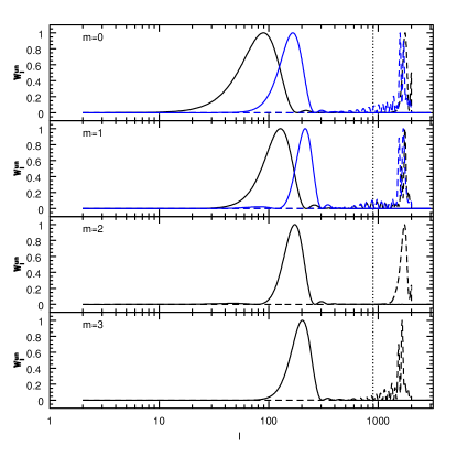
Figure 2: Window functions for $E$ and $B$ modes for a hypothetical experiment in which measurements are made on a spherical cap. The dashed lines show the leakage of $E$ into $B$ or vice versa. The leakage is caused by pixelization and appears at the Nyquist scale, indicated by the vertical dotted line. For further details, see ref. bunnetal , from which this figure is taken.

In the limit of a map with infinitely dense pixelization, the $E$/$B$/ambiguous decomposition depends only on the geometry of the observed region. Orthonormal bases for the pure and ambiguous subspaces can be found by finding eigenfunctions of a certain differential operator bunnetal . As expected from the heuristic argument above, the amount of information lost to ambiguous modes is largest on the largest observable scales. To be specific, the ratio $N_{\rm amb}/N_{\rm pure}$ of ambiguous to pure modes is $\sim 1$ on the largest observed scales and decreases as $1/k$ with increasing wavenumber $k$.

Pixelization also causes mixing of $E$ and $B$ modes. We can understand this intuitively by imagining a survey that observes a square region of sky. Pixelization introduces a Nyquist wavenumber $k_{\rm Ny}$, such that all modes with wavevector components greater than $k_{\rm Ny}$ are aliased to modes with wavenumbers less than the Nyquist value. This aliasing completely shuffles the directions of the wavevectors, so it leads to essentially complete $E$/$B$ mixing. In particular, consider an $E$ mode with wavenumber close to the Nyquist value. The mean-square amplitude of this mode will be $C_{k_{\rm NY}}^{E}e^{-\sigma_{b}^{2}k_{\rm Ny}^{2}}$, where $\sigma_{b}$ is the Gaussian beam width. Due to aliasing, a significant fraction of the power in this mode will appear to be part of a $B$ mode with mean-square amplitude $C_{k}^{B}$ for some small wavenumber $k$. To avoid significant degradation of $B$ mode measurements, therefore, we should pixelize on a fine enough scale (that is, make $k_{\rm Ny}$ large enough) to satisfy the inequality

$$e^{-\sigma_{b}^{2}k_{\rm Ny}^{2}}<{C_{k}^{B}\over C_{k_{\rm Ny}}^{E}}.$$ (1)

This typically implies oversampling the beam of the experiment by a factor of $\sim 3$-$4$.

Figure 2 shows an example of the effects of pixelization on the window functions for supposedly pure $E$ and $B$ modes. The dashed curves show the “leakage” window functions, that is, the contribution of $E$ to a supposed $B$ mode and vice versa. The leakage appears suddenly at a particular scale, which is the Nyquist scale for the experiment in question. For further details, see ref. bunnetal .

3 Efficient real-space decomposition

Finding a basis of orthonormal pure and ambiguous modes is in principle straightforward, but for a map with a large number of pixels and/or a complicated geometry, it can be computationally expensive. In this section, I sketch a method for decomposing a map into pure $E$, pure $B$, and ambiguous maps without finding such a basis. The procedure consists of two steps:

1. Do a naïve separation of the map into $E$ and $B$ components, without worrying about the presence of ambiguous modes. At the end of this step, the original map will be written as the sum of two terms, one of which consists of pure $E$ and ambiguous modes, and one of which consists of pure $B$ and ambiguous modes.

2. “Purify” each of the two maps found in step 1.

Step 1 can be done in a wide variety of ways. In the flat-sky approximation, one way is to pad the map out to a rectangular shape (using zeroes or any other values for $Q,U$ in the padded regions). One then performs a fast Fourier transform on the padded map, performs the $E$/$B$ decomposition trivially in Fourier space, and transforms back. The resulting $E$ map will consist entirely of $E$ modes, although not necessarily of pure $E$ modes – that is, it will be a combination of $E$ and ambiguous modes. If the flat-sky approximation is not appropriate, the same can be done in spherical harmonic space, e.g., with HEALPix healpix .

We must now “purify” each of these two maps. In an earlier work bunnmn , I described one way to do this, based on Green functions; however, that method is not very efficient in practice. I will now sketch a simpler and more efficient method.

Let us recall some mathematical properties of the ambiguous modes LCT ; bunnetal . Any $E$ mode (pure or not) can be written in terms of a scalar potential $\psi$:

$${\bf P}={\bf D}_{E}\psi.$$ (2)

Here ${\bf P}$ represents the spin-two field $(Q,U)$, and ${\bf D}_{E}$ is a certain second-order differential operator. Furthermore, all $B$ modes satisfy the equation

$${\bf D}_{E}^{\dagger}\cdot{\bf P}=0.$$ (3)

Since an ambiguous mode is both an $E$ mode and a $B$ mode, it can be derived from a potential $\psi$ that satisfies the differential equation ${\bf D}_{E}^{\dagger}\cdot{\bf D}_{E}\psi=0$, which is equivalent to

$$\nabla^{2}(\nabla^{2}+2)\psi=0.$$ (4)

Solutions to this equation are uniquely determined by the values of $\psi$ and its derivatives on the boundary of the region, which can be expressed in terms of the data contained in the $Q,U$ maps. Furthermore, equation (4) can be solved numerically quite efficiently, for example by relaxation methods.

(a) (b) (c)

(d) (e) (f)

Figure 3: Example of real-space $E$/$B$/ambiguous decomposition. The original map (a) was decomposed into $E$ and $B$ components (b,c). The $B$ component was then separated into ambiguous (d) and pure (e) parts. For comparison, the $B$ component of the true, original map is shown in panel (f). Because the amplitudes of the $B$ modes was chosen to be lower than the $E$ modes by a factor 10, the polarizations in panels (e,f) have been multiplied by 10.

Figure 3 shows an example of this procedure.

This “purification” method may prove useful in conjunction with other CMB analysis methods, such as the pseudo-$C_{l}$ method. One proposed way of applying this method to polarization data smithzal is to apply the “curl” differential operator ${\bf D}_{B}$ to the original sky map before calculating pseudo-$C_{l}$’s. Because all $E$ modes (pure or otherwise) are mapped to zero by this operator, this has the effect of projecting down onto the pure $B$ subspace. Because this approach involves taking derivatives of noisy, pixelized data, careful apodization of the weight functions used in calculating the pseudo-$C_{l}$’s is required. The authors of this work have shown how to solve this problem. However, it is tempting to speculate that the method would be easier to implement and more transparent if differentiation of the data could be avoided from the beginning. It may be possible to achieve this goal by performing the projection described in this section instead of applying the operator ${\bf D}_{B}$. Both procedures have the effect of projecting down to the pure $B$ subspace, but the procedure described here results in the actual pure $B$ map, rather than a second derivative of it. I wish to emphasize that this proposal is at this stage largely speculation; this approach requires further investigation.

4 Discussion

Separation into $E$ and $B$ components will be an essential step in the analysis of future CMB polarization experiments, particularly those focused on characterization of the weaker $B$ modes. Fortunately, the $E$/$B$ separation problem does not pose major data analysis challenges: methods for performing the separation in real space are known, as are methods for calculating power spectrum estimates on the original maps that take full account of the presence of ambiguous modes (e.g., smithzal ).

When designing and optimizing experiments, it is important to consider the degree to which $B$ mode information is lost to ambiguous modes. In general, the ambiguous modes primarily affect the largest observable scales in any given experiment. Unfortunately, these are also the scales where the signal-to-noise is highest. Because the ambiguous modes are caused by conditions on the boundary of the map, the most efficient survey designs are those with short boundaries (i.e., rounder is better). Furthermore, aliasing of modes above the Nyquist frequency strongly mixes the $E$ and $B$ components. As a result, oversampling of the beam is even more important in polarization experiments than in temperature anisotropy measurements.

Although it is always possible to construct a basis of orthonormal modes that implement the separation into $E,B$, and ambiguous components, such a construction is cumbersome and computationally expensive in practice. I have sketched a procedure for “purifying” the components of a data set in real space without the construction of such a basis. This approach may be useful when using estimators such as the pseudo-$C_{l}$’s, although further research in this area is needed.

Finally, I would like to comment briefly on the tradeoffs between interferometric and single-dish imaging experiments. Interferometric visibilities are well-localized in Fourier space, and hence they provide sharp power spectrum estimates parkng . Since, as we have seen above, $E$/$B$ mixing is closely connected with resolution in Fourier space, we might expect interferometers to be better than imaging experiments in this regard as well. Further research is needed to quantitatively assess this claim, however.

An individual pair of visibilities $(V_{Q},V_{U})$ from a single interferometer baseline does contain separable information about $E$ and $B$ modes, whereas no $E,B$ information can be extracted from a single pixel of an imaging experiment. For relatively short baselines, relatively little $B$ information can be extracted from a single visibility pair, however, because there is significant $E$/$B$ mixing. In practice, $B$ information can be extracted from a single visibility only if $\overline{s^{2}}<(C_{B}/C_{E})\sim 10^{-2}$, where $\overline{s^{2}}$ is a measure of the spread in wavevector directions probed by the given baseline polsys . This inequality is achieved when the antenna separation is at least $\sim 4$ times the antenna diameter. Since CMB interferometers are traditionally close-packed, many baselines are shorter than this. $E$/$B$ separation is still possible for these short baselines, but it requires dense sampling of the visibility plane and/or mosaicking bunnwhite to improve Fourier space resolution.

This work was supported by National Science Foundation Awards AST-0098048 and AST-0507395.

References

- [1] Zaldarriaga M and Seljak U 1997 Phys. Rev. D 55 1830–1840 (Preprint arXiv:astro-ph/9609170)
- [2] Seljak U and Zaldarriaga M 1997 Phys. Rev. Lett. 78 2054–2057 (Preprint arXiv:astro-ph/9609169)
- [3] Kamionkowski M, Kosowsky A and Stebbins A 1997 Phys. Rev. Lett. 78 2058–2061 (Preprint arXiv:astro-ph/9609132)
- [4] Kamionkowski M, Kosowsky A and Stebbins A 1997 Phys. Rev. D 55 7368–7388 (Preprint arXiv:astro-ph/9611125)
- [5] Lewis A, Challinor A and Turok N 2002 Phys. Rev. D 65 023505–+ (Preprint arXiv:astro-ph/0106536)
- [6] Bunn E F 2002 Phys. Rev. D 65 043003–+ (Preprint arXiv:astro-ph/0108209)
- [7] Bunn E F, Zaldarriaga M, Tegmark M and de Oliveira-Costa A 2003 Phys. Rev. D 67 023501–+ (Preprint arXiv:astro-ph/0207338)
- [8] Górski K M, Hivon E, Banday A J, Wandelt B D, Hansen F K, Reinecke M and Bartelmann M 2005 ApJ 622 759–771 (Preprint arXiv:astro-ph/0409513)
- [9] Bunn E F 2003 New Astron. Rev. 47 987–994 (Preprint arXiv:astro-ph/0306003)
- [10] Smith K M and Zaldarriaga M 2007 Phys. Rev. D 76 043001–+ (Preprint arXiv:astro-ph/0610059)
- [11] Park C G and Ng K W 2004 ApJ 609 15–21 (Preprint arXiv:astro-ph/0304167)
- [12] Bunn E F 2007 Phys. Rev. D 75 083517–+ (Preprint arXiv:astro-ph/0607312)
- [13] Bunn E F and White M 2007 ApJ 655 21–29 (Preprint arXiv:astro-ph/0606454)