Low temperature thermal conductivity in a $d$-wave superconductor with coexisting charge order: Effect of self-consistent disorder and vertex corrections

Abstract

Given the experimental evidence of charge order in the underdoped cuprate superconductors, we consider the effect of coexisting charge order on low-temperature thermal transport in a $d$-wave superconductor. Using a phenomenological Hamiltonian that describes a two-dimensional system in the presence of a ${\bf Q}=(\pi,0)$ charge density wave and $d$-wave superconducting order, and including the effects of weak impurity scattering, we compute the self-energy of the quasiparticles within the self-consistent Born approximation, and calculate the zero-temperature thermal conductivity using linear response formalism. We find that vertex corrections within the ladder approximation do not significantly modify the bare-bubble result that was previously calculated. However, self-consistent treatment of the disorder does modify the charge-order-dependence of the thermal conductivity tensor, in that the magnitude of charge order required for the system to become effectively gapped is renormalized, generally to a smaller value.

I Introduction

The superconducting phase of the cuprate superconductors exhibits $d$-wave pairing symmetry.har01 As such, there exist four nodal points on the two-dimensional Fermi surface at which the quasiparticle excitations are gapless, and quasiparticles excited in the vicinity of a node behave like massless Dirac fermions.lee02 ; alt01 ; ore01 . The presence of impurities enhances the density of states at low energygor01 resulting in a universal limit $(T\rightarrow 0,~{}\Omega\rightarrow 0)$ where the thermal conductivity is independent of disorder.lee01 ; hir01 ; hir02 ; hir03 ; graf01 ; sen01 ; dur01 Calculations have shown that the thermal conductivity retains this universal character even upon the inclusion of vertex corrections.dur01 Experiments have confirmed the validity of this quasiparticle picture of transport by observing their universal-limit contribution to the thermal conductivity, and thereby measuring the anisotropy of the the Dirac nodes, $v_{f}/v_{\Delta}$.tai01 ; chi01 ; chi02 ; nak01 ; pro01 ; sut01 ; hil01 ; sun01 ; sut02 ; haw01 ; sun02

For some time, there has been significant interest kiv01 ; pod01 ; li01 ; che01 ; seo01 in the idea of additional types of order coexisting with $d$-wave superconductivity (dSC) in the cuprates. And in recent years, as the underdoped regime of the phase diagram has been explored in greater detail, evidence of coexisting order has grown substantially kiv01 . Particularly intriguing has been the evidence of checkerboard charge order revealed via scanning tunnelling microscopy (STM) experiments. hof01 ; hof02 ; how01 ; ver01 ; mce01 ; han01 ; mis01 ; mce02 ; koh01 ; boy01 ; han02 ; pas01 ; wis01 ; koh02

And if charge order coexists with $d$-wave superconductivity in the underdoped cuprates, it begs the question of how the quasiparticle excitation spectrum is modified. Previous work ber01 has shown that even with the addition of a charge or spin density wave to the dSC hamiltonian, the low-energy excitation spectrum remains gapless as long as a harmonic of the ordering vector does not nest the nodal points of the combined hamiltonian. However, if the coexisting order is strong enough, the nodal points can move to $k$-space locations where they are nested by the ordering vector, at which point the excitation spectrum becomes fully gapped. par01 ; gra01 ; voj01

Such a nodal transition should have dramatic consequences for low-temperature thermal transport, the details of which were studied in Ref. dur02, . That paper considered the case of a conventional $s$-wave charge density wave (CDW) of wave vector $\mathbf{Q}=(\pi,0)$ coexisting with $d$-wave superconductivity. It showed that the zero-temperature thermal conductivity vanishes, as expected, once charge order is of sufficient magnitude to gap the quasiparticle spectrum. In addition, the dependence of zero-temperature thermal transport was calculated and revealed to be disorder-dependent. Hence, in the presence of charge order, the universal-limit is no longer universal. This result is in line with the results of recent measurements hus01 ; tak01 ; sun05 ; and01 ; sun03 ; sun04 ; haw02 of the underdoped cuprates, as well as other calculations gus01 ; ander01 .

We extend the work of Ref. dur02, herein. We consider the same physical system, but employ a more sophisticated model of disorder that includes the effects of impurity scattering within the self-consistent Born approximation. We find that this self-consistent model of disorder requires that off-diagonal components be retained in our matrix self-energy. These additional components lead to a renormalization of the critical value of charge order beyond which the thermal conductivity vanishes. Furthermore, we include the contribution of vertex corrections within our diagrammatic thermal transport calculation. While vertex corrections become more important as charge order increases, especially for long-ranged impurity potentials, we find that for reasonable parameter values, they do not significantly modify the bare-bubble result.

In Sec. II, we introduce the model hamiltonian of the dSC+CDW system, describe the effect charge ordering has on the nodal excitations, and present our model for disorder. In Sec. III.1, a numerical procedure for computing the self-energy within the self-consistent Born approximation is outlined. The results of its application in the relevant region of parameter space are presented in Sec. III.2. In Sec. IV, we calculate the thermal conductivity using a diagrammatic Kubo formula approach, including vertex corrections within the ladder approximation. An analysis of the vertex-corrected results and a calculation of the clean-limit thermal conductivity is presented in Sec. V. Also in this section, we discuss how our self-consistent model of disorder renormalizes the nodal transition point, the value of charge order parameter at which the nodes effectively vanish. Conclusions are presented in Sec. VI.

II Model

We employ the phenomenological hamiltonian of Ref. dur02, in order to calculate the low-temperature thermal conductivity of the fermionic excitations of a $d$-wave superconductor with a $\mathbf{Q}=(\pi,0)$ charge density wave, in the presence of a small but nonzero density of point-like impurity scatterers. The presence of $d$-wave superconducting order contributes a term to the hamiltonian

$$H_{dSC}=\frac{1}{2}\sum_{k\alpha}\Big{(}\epsilon_{k}c_{k\alpha}^{\dagger}c_{k\alpha}+\Delta_{k}c_{k\alpha}^{\dagger}c_{-k\beta}^{\dagger}\Big{)}+\mathrm{h.c.}$$ (1)

where $\epsilon_{k}$ is a typical tight-binding dispersion, and $\Delta_{k}$ an order parameter of $d_{x^{2}-y^{2}}$ symmetry. Due to the $d$-wave nature of the gap, nodal excitations exist in the $(\pm\pi,\pm\pi)$ directions with respect to the origin. The locations of these nodes in the absence of charge ordering are close to the points $(\pm\pi/2,\pm\pi/2)$, and are denoted with white dots in Fig. 1. These low energy excitations are massless anisotropic Dirac fermions. That is, the electron dispersion and pair function are linear functions of momentum in the vicinity of these nodal locations. We will refer to the slopes of the electron dispersion and pair function, defined by $\mathbf{v}_{f}\equiv\frac{\partial\epsilon_{k}}{\partial\bf{k}}$ and $\mathbf{v}_{\Delta}\equiv\frac{\partial\Delta_{k}}{\partial\bf{k}}$, as the Fermi velocity and gap velocity respectively. The energy of the quasiparticles in the vicinity of the nodes is given by $E_{k}=\sqrt{v_{f}^{2}k_{1}^{2}+v_{\Delta}^{2}k_{2}^{2}}$, where $k_{1}$ and $k_{2}$ are the momentum displacements (from the nodes) in directions perpendicular to and parallel to the Fermi surface. The universal-limit $(T\rightarrow 0,\Omega\rightarrow 0)$ transport properties of these quasiparticles was explored in Ref. dur01, .

While experiments have revealed evidence of a number of varieties of spin and charge order, the system described in this paper will be restricted to the addition of a site-centered charge density wave of wave vector $\mathbf{Q}=(\pi,0)$, which contributes a term to the hamiltonian

$$H_{CDW}=\sum_{k\alpha}a_{k}c_{k\alpha}^{\dagger}c_{k+Q\alpha}+\mathrm{h.c.}$$ (2)

The charge density wave doubles the unit cell, reducing the Brillouin zone to the shaded portion seen in Fig. 1.

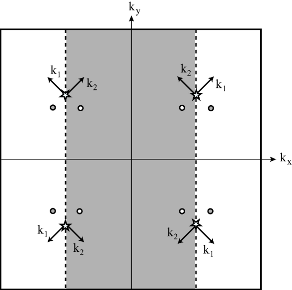
Figure 1: Illustrated is the Brillouin zone for our model, reduced to the shaded region by unit-cell-doubling charge order. The $\psi=0$ nodal locations are illustrated by white dots. They are displaced by a distance $k_{0}$ from the $(\pm\frac{\pi}{2},\pm\frac{\pi}{2})$ points (stars). As the charge density wave’s amplitude increases, the location of the gapless excitations evolves along curved paths toward the $(\pm\frac{\pi}{2},\pm\frac{\pi}{2})$ points, until $\psi$ reaches $\psi_{c}$, when the spectrum becomes gapped because the nodes are nested by the charge density wave-vector. The gray dots depict the images of the nodes in the second reduced Brillouin zone.

Restricting summations over momentum space to the reduced Brillouin zone, and invoking the charge density wave’s time-reversal symmetry and commensurability with the reciprocal lattice, we are able to write the hamiltonian as

$$H = \sum_{k}\Psi^{\dagger}_{k}H_{k}\Psi\hskip 10.0ptH_{k}=H^{dSC}_{k}+H^{CDW}_{k},$$ (3)

where

$$H_{k}=\begin{pmatrix}\epsilon_{k}&\Delta_{k}&\psi&0\\ \Delta_{k}&-\epsilon_{k}&0&-\psi\\ \psi&0&\epsilon_{k+Q}&\Delta_{k+Q}\\ 0&-\psi&\Delta_{k+Q}&-\epsilon_{k+Q}\end{pmatrix},$$ (4)

is a matrix in the basis of extended-Nambu vectors,

$$\Psi_{k}=\begin{pmatrix}c_{k\uparrow}\\ c^{\dagger}_{-k\downarrow}\\ c_{k+Q\uparrow}\\ c^{\dagger}_{-k-Q\downarrow}\end{pmatrix}\hskip 10.0pt\Psi^{\dagger}_{k}=\begin{pmatrix}c^{\dagger}_{k\uparrow}&c_{-k\downarrow}&c^{\dagger}_{k+Q\uparrow}&c_{-k-Q\downarrow}\end{pmatrix}$$ (5)

and $\psi$ represents the constant value taken at the nodes by the charge density wave order parameter $A_{k}=a_{k}+a_{k+Q}^{*}$.

The onset of the charge order modifies the energy spectrum of the clean hamiltonian so that the locations of the nodes evolve along curved paths towards the $(\pm\frac{\pi}{2},\pm\frac{\pi}{2})$ points at the edges of the reduced Brillouin zone, as was noted in Ref. par01, . “Ghost” nodes, their images in what is now the second reduced Brillouin zone, evolve the same way, until the charge density wave is strong enough that the nodes and ghost nodes collide at those $(\pm\pi/2,\pm\pi/2)$ points. When that occurs, $\mathbf{Q}$ nests two of the nodes, gapping the spectrum so that low temperature quasiparticle transport is no longer possible. We define the value of $\psi$ at which this occurs as $\psi_{c}$. Due to the nodal properties of the quasiparticles, all functions of momentum space $\mathbf{k}$ can be parametrized in terms of a node index $j$, and local coordinates $p_{1}$ and $p_{2}$ in the vicinity of each node. We choose to parametrize our functions using symmetrized coordinates centered at $(\pm\pi/2,\pm\pi/2)$,

$$\epsilon_{k} = \psi_{c}+\beta p_{1}\hskip 40.0pt\Delta_{k}=\frac{1}{\beta}p_{2}$$

$$\epsilon_{k+Q} = \psi_{c}+\beta p_{2}\hskip 40.0pt\Delta_{k+Q}=\frac{1}{\beta}p_{1}$$ (6)

where we have rescaled $\sqrt{v_{f}v_{\Delta}}k_{1}=p_{1}$ for the coordinate normal to Fermi surface, $\sqrt{v_{f}v_{\Delta}}k_{2}=p_{2}$ for the coordinate parallel to Fermi surface, and introduced the definition $\beta\equiv\sqrt{\frac{v_{f}}{v_{\Delta}}}$. In this coordinate system, the displacement of the original node locations from the collision points is given by $\psi_{c}$. A sum over momentum space is therefore performed by summing over nodes, and integrating over each node’s contribution, as follows.

$$\sum_{k}f(\mathbf{k})\rightarrow\frac{1}{2}\sum_{j=1}^{4}\int\frac{\mathrm{d}^{2}p}{4\pi^{2}v_{f}v_{\Delta}}f^{(j)}(p_{1},p_{2})$$

$$=\frac{1}{8\pi^{2}v_{f}v_{\Delta}}\sum_{j=1}^{4}\int_{-p_{0}}^{p_{0}}\mathrm{d}p_{1}\int_{-p_{0}}^{p_{0}}\mathrm{d}p_{2}\,\,f^{(j)}(p_{1},p_{2})$$ (7)

where the factor of $\frac{1}{2}$ comes from extending the integrals to all $p_{1}$ and $p_{2}$, rather than just the shaded part depicted in Fig. 1, and $p_{0}$ is a high-energy cutoff.

At sufficiently low temperatures, the thermal conductivity is dominated by the nodal excitations, since phonon modes are frozen out, and other quasiparticles are exponentially rare. Using this fact, we can calculate the low temperature thermal conductivity of the system using linear response formalism.

We incorporate disorder into the model by including scattering events from randomly distributed impurities. Because the quasiparticles are nodal, only limited information about the scattering potential is needed, in particular, the amplitudes $V_{1},V_{2}$ and $V_{3}$, for intra-node, adjacent node, and opposite node scattering respectively, as explained in Ref. dur01, . We calculate the thermal conductivity using linear response formalism, wherein we obtain the retarded current-current correlation function by analytic continuation of the corresponding Matsubara correlator mah01 ; Fetter .

In Ref. dur02, , using a simplified model for disorder, where the self-energy was assumed to be a negative imaginary scalar, the thermal conductivity was calculated as a function of $\psi$, and found to vanish for $\psi>\psi_{c}$. We now improve upon that result by calculating the self-energy within the self-consistent Born approximation, and by including vertex corrections within the ladder approximation in our calculation of the thermal conductivity.

III Self-Energy

III.1 SCBA Calculation

Within the self-consistent Born approximation (SCBA), the self-energy tensor is given by

$$\widetilde{\Sigma}(\mathbf{k},\omega)=n_{\mathrm{imp}}\sum_{k^{\prime}}\left|V_{kk^{\prime}}\right|^{2}(\widetilde{\sigma_{0}\otimes\tau_{3}})\widetilde{\mathcal{G}}(\mathbf{k},\omega)(\widetilde{\sigma_{0}\otimes\tau_{3}})$$ (8)

where $n_{\mathrm{imp}}$ is the impurity density and $\widetilde{V}_{kk^{\prime}}=V_{kk^{\prime}}(\widetilde{\sigma_{0}\otimes\tau_{3}})$ accompanies each scattering event, as seen in Fig. 2. The tilde signifies an operator in the extended-Nambu basis, and the $\sigma$’s and $\tau$’s are Pauli matrices in charge-order-coupled and particle-hole spaces respectively.

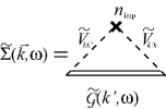
Figure 2: Feynman diagram depicting self-energy in the self-consistent Born approximation. The double line represents the dressed propagator, the dashed line represents the interaction with the impurity, and the cross represents the impurity density.

$\widetilde{\mathcal{G}}(\mathbf{k},\omega)$ is the full Green’s function, whose relation to the bare Green’s function $\widetilde{\mathcal{G}}_{0}(\mathbf{k},\omega)$ and the self-energy $\widetilde{\Sigma}(\mathbf{k},\omega)$ is given by Dyson’s equation

$$\widetilde{\mathcal{G}}(\mathbf{k},\omega)=(\widetilde{\mathcal{G}}^{-1}_{0}(\mathbf{k},\omega)-\widetilde{\Sigma}(\mathbf{k},\omega))^{-1},$$ (9)

the bare Green’s function having been determined by

$$\widetilde{\mathcal{G}}_{0}(\mathbf{k},\omega)=(\omega\widetilde{\openone}-\widetilde{H}_{k})^{-1}.$$ (10)

Eq. (8) and Eq. (9) define a set of integral equations for the self-energy $\widetilde{\Sigma}(\mathbf{k},\omega)$. For the calculation of the universal-limit thermal conductivity, it is sufficient to find the zero-frequency limit of the self-energy. In its present form, $\widetilde{\Sigma}$ has 32 real components. Below, we demonstrate that this number can be reduced further to six components.

If we write the Green’s function as

$$\widetilde{\mathcal{G}}(\mathbf{k},\omega)=\frac{1}{\mathcal{G}_{den}}\left(\begin{array}[]{cc}\mathcal{G}_{A}&\mathcal{G}_{B}\\ \mathcal{G}_{C}&\mathcal{G}_{D}\end{array}\right),$$ (11)

where

$$\mathcal{G}_{\alpha}=\sum_{i=0}^{3}\mathcal{G}_{\alpha i}\tau_{i}$$ (12)

then the self-energy can be written as the set of 16 complex equations (for $\alpha=\{A,B,C,D\}$, $i=\{0,1,2,3\}$)

$$\Sigma_{\alpha i} = n_{\mathrm{imp}}\sum_{k^{\prime}}\left|V_{kk^{\prime}}\right|^{2}\frac{\xi_{i}}{\mathcal{G}_{den}}\mathcal{G}_{\alpha i}$$ (13)

$$= \xi_{i}c\int\mathrm{d}^{2}p\frac{\mathcal{G}_{\alpha i}\left(p_{1},p_{2}\right)}{\mathcal{G}_{den}\left(p_{1},p_{2}\right)}$$

where $\xi_{i}=\left\{\begin{array}[]{c}+1,\,i=0,3\\ -1,\,i=1,2\end{array}\right\}$, $c=\frac{n_{i}(V_{1}^{2}+2V_{2}^{2}+V_{3}^{2})}{8\pi^{2}v_{f}v_{\Delta}}$, and the final line is realized by using the notation of Eq. (II) and Eq. (II) and completing the sum over nodes. From the symmetries of the hamiltonian, we are able to ascertain certain symmetries the bare Green’s function will obey, specifically,

$$\mathcal{G}^{(0)}_{A0}(p_{2},p_{1}) = \mathcal{G}^{(0)}_{D0}\left(p_{1},p_{2}\right)$$ (14)

$$\mathcal{G}^{(0)}_{A1}(p_{2},p_{1}) = \mathcal{G}^{(0)}_{D1}\left(p_{1},p_{2}\right)$$

$$\mathcal{G}^{(0)}_{A3}(p_{2},p_{1}) = \mathcal{G}^{(0)}_{D3}\left(p_{1},p_{2}\right)$$

$$\mathcal{G}^{(0)}_{B0}(p_{2},p_{1}) = \mathcal{G}^{(0)}_{C0}\left(p_{1},p_{2}\right)$$

$$\mathcal{G}^{(0)}_{B1}(p_{2},p_{1}) = \mathcal{G}^{(0)}_{C1}\left(p_{1},p_{2}\right)$$

$$\mathcal{G}^{(0)}_{B2}(p_{2},p_{1}) = \mathcal{G}^{(0)}_{C2}\left(p_{1},p_{2}\right)$$

$$\mathcal{G}^{(0)}_{B3}(p_{2},p_{1}) = \mathcal{G}^{(0)}_{C3}\left(p_{1},p_{2}\right)$$

$$\mathcal{G}^{(0)}_{\mathrm{den}}(p_{2},p_{1}) = \mathcal{G}^{(0)}_{\mathrm{den}}(p_{1},p_{2})$$

In addition, the realization that the integration is also symmetric with respect to exchange of $p_{1}$ and $p_{2}$, coupled with these symmetries, lead to relations for self-energy components

$$\Sigma_{Ai} = \Sigma_{Di}$$ (15)

$$\Sigma_{Bi} = \Sigma_{Ci}\hskip 40.0pti=0,1,2,3$$

$$\Sigma_{B2} = \Sigma_{C2}=0$$

so that we see a reduction from 32 components of the self-energy to 6 independent components:$\{\Sigma_{\alpha i}\}\equiv\{\Sigma_{A0},\Sigma_{A1},\Sigma_{A3},\Sigma_{B0},\Sigma_{B1},\Sigma_{B3}\}$. A self-consistent self-energy must therefore satisfy 6 coupled integral equations given by Eq. (13).

The self-consistent calculation of the self-energy proceeds by applying the following scheme: First, a guess is made as to which self-energy components will be included. The full Green’s function corresponding to such a self-energy is then obtained from Dyson’s equation, Eq. (9). The quantitative values of the $\Sigma_{\alpha i}$’s are then determined as follows: An initial guess for the quantitative values of each of the $\Sigma_{\alpha i}$’s is made, and the six integrals of Eq. (13) are computed numerically, which provides the next set of guesses for $\{\Sigma_{\alpha i}\}$. This process is repeated until a stable solution is reached. Finally, the resulting solutions must be checked that they are consistent with the initial guess for the form of $\widetilde{\Sigma}$. If they are, the self-consistent calculation is complete.

We begin with the simplest assumption, that $\widetilde{\Sigma}^{(1)}(\omega)=-i\Gamma_{0}\widetilde{(\sigma_{0}\otimes\tau_{0})}$, where $\Gamma_{0}$ is the zero-frequency limit of the scattering rate. The superscript indicates that this is the first guess for $\widetilde{\Sigma}$. The Green’s function components are computed, which gives the explicit form of Eq. (8). Upon evaluating the numerics, it is seen that this first iteration generates a nonzero (real and negative) term for $\Sigma_{B1}$. So, the diagonal self-energy assumption turns out to be inconsistent, in contrast to the situation for $\psi=0$. We then modify our guess, assuming self-energy of the form $\widetilde{\Sigma}^{(2)}=-i\Gamma_{0}\widetilde{(\sigma_{0}\otimes\tau_{0})}-B_{1}\widetilde{(\sigma_{1}\otimes\tau_{1})}$. The Green’s function is computed again, using Dyson’s equation, and the self-energy equations are obtained explicitly. It is noted that the symmetries of Eq. (14) still hold. Again, the equations (13) are solved iteratively; the result is a non-zero $\Sigma_{B3}$ component as well. Once again, the Green’s functions are modified to incorporate this term, and the iterative scheme is applied. Calculation of the self-energy based on the assumption

$$\widetilde{\Sigma}^{(3)}=-i\Gamma_{0}\widetilde{(\sigma_{0}\otimes\tau_{0})}-B_{1}\widetilde{(\sigma_{1}\otimes\tau_{1})}-B_{3}\widetilde{(\sigma_{1}\otimes\tau_{3})}$$

$$\Gamma_{0},B_{1},B_{3}>0$$ (16)

generates $\Gamma_{0}$, $B_{1}$, and $B_{3}$ that are much larger than any remaining terms, and hence provides the self-consistent values of $\Sigma_{A0},\Sigma_{B1}$ and $\Sigma_{B3}$. A plot of the 6 components of $\widetilde{\Sigma}$ is displayed in Fig. 3 for a representative parameter set, where we see that the three terms of the ansatz are indeed dominant. For the remainder of this paper, the effect of the $\Sigma_{A1}$, $\Sigma_{A3}$ and $\Sigma_{B0}$ components will be ignored. The self-consistent Green’s functions are provided in Appendix A, while additional details of the self-energy calculation are discussed in Appendix B.

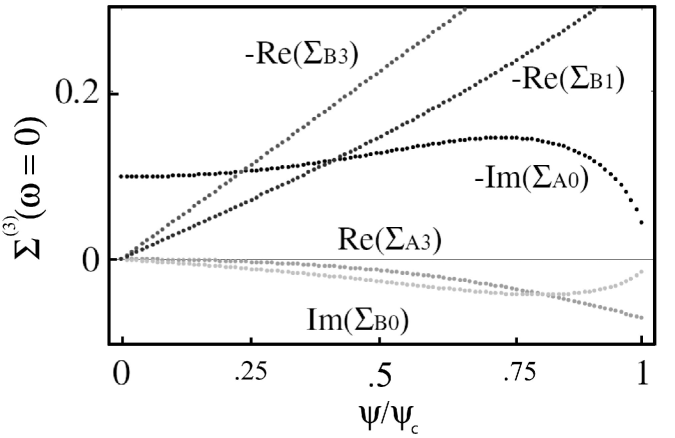
Figure 3: Components of self-energy computed using iterative procedure described in Sec. III.1. The third iteration self-energy, $\widetilde{\Sigma}^{(3)}$, is shown here. The dominance of $\Gamma_{0}=-\mathrm{Im}(\Sigma_{A0}),B_{1}=-\mathrm{Re}(\Sigma_{B1})$, and $B_{3}=-\mathrm{Re}(\Sigma_{B3})$ over other components establishes this third iteration as yielding the (approximately) self-consistent value of the self-energy. $\Sigma_{A1}$ and $\Sigma_{A3}$ overlap.

III.2 SCBA Results

In order to discuss the numerical results contained in this paper, it is necessary to make a note about the units employed. The following discussion of units applies as well to the numerical analysis of the results of the thermal conductivity calculation in Sec. V. Because we are studying the evolution of the system with respect to increasing CDW order parameter $\psi$, we wish to express energies in units of $\psi_{c}$, the value of $\psi$ which gaps the clean system. In order to do this, the cutoff $p_{0}$ is fixed such that the Brillouin zone being integrated over in Eq. (II) has the correct area. In this way, $p_{0}$ sets the scale of the product $v_{f}v_{\Delta}$; a parameter $\beta\equiv\sqrt{\frac{v_{f}}{v_{\Delta}}}$ is defined to represent the velocity anisotropy. Then, $\frac{p_{0}}{\psi_{c}}=\frac{\pi}{2a}\sqrt{v_{f}v_{\Delta}}$, so that we may eliminate the frequently occurring parameter $4\pi v_{f}v_{\Delta}$ by expressing lengths in units of $\frac{4}{\sqrt{\pi}}a\approx 2.25a$. Impurity density $n_{\mathrm{imp}}$ is thus recast in terms of impurity fractions $z$ according to $n_{\mathrm{imp}}=\frac{16}{\pi}z$. Finally, the parameters of the scattering potential are recast in terms of their anisotropy. We define $V_{2}\equiv R_{2}V_{1}$ and $V_{3}\equiv R_{3}V_{1}$.

With these modifications, the original set of parameters, $\{n_{i},V_{1},V_{2},V_{3},v_{f},v_{\Delta},p_{0},\psi,\psi_{c}\}$ is reduced to $\{z,V_{1},R_{2},R_{3},\beta,p_{0},\psi\}$. For the work contained herein, the cutoff $p_{0}$ is fixed at $p_{0}=100$. The self-energy in the self-consistent Born approximation was computed for different scattering potentials as a function of impurity fraction and CDW order parameter $\psi$. Since it was found that three of the components, $\Sigma_{A0}$, $\Sigma_{B1}$ and $\Sigma_{B3}$, dominate over the others, we will subsequently analyze only those three components, referring to their magnitudes as $\Gamma_{0}$, $B_{1}$, and $B_{3}$ respectively.

As $z\rightarrow 0$, the Green’s functions become impossibly peaked from a numerical point of view. For sufficiently large $z$, depending on the strength of the scatterers, the Born approximation breaks down. Given a scattering strength of $V_{1}=110$, cutoff $p_{0}=100$, scattering potentials that fall off slowly in $k$-space and velocity anisotropy ratios $\beta\equiv\sqrt{v_{f}/v_{\Delta}}={1,2,3,4}$, this puts the range of $z$ in which our numerics may be applied at roughly between one half and one percent.

Some results for $\widetilde{\Sigma}(\psi)$, for several values of $z$, are shown in Figs. 4 and 5. These plots correspond to the same parameters, except that Fig. 4 illustrates the $v_{f}=v_{\Delta}$ case, and Fig. 5 illustrates $v_{f}=16v_{\Delta}$. In all cases it is seen that

$$B_{1}(\psi,z)\simeq b_{1}(z)\psi$$

$$B_{3}(\psi,z)\simeq b_{3}(z)\psi$$ (17)

where the dependence of $B_{1}$, $B_{3}$, $b_{1}$, and $b_{3}$ on the remaining parameters is implicit. For much of the parameter space sampled, $\Gamma_{0}$ does not have much $\psi$ dependence, except that it typically rises and then falls to zero at some sufficiently large $\psi<\psi_{c}$. This feature will be revisited in Sec. V, wherein it is explained that this vanishing scattering rate coincides with vanishing thermal conductivity, and corresponds to the point at which the system becomes effectively gapped and our nodal approximations break down. The value of $\psi$ at which this occurs depends on the entire set of parameters used, and will be referred to as $\psi_{c}^{*}$.

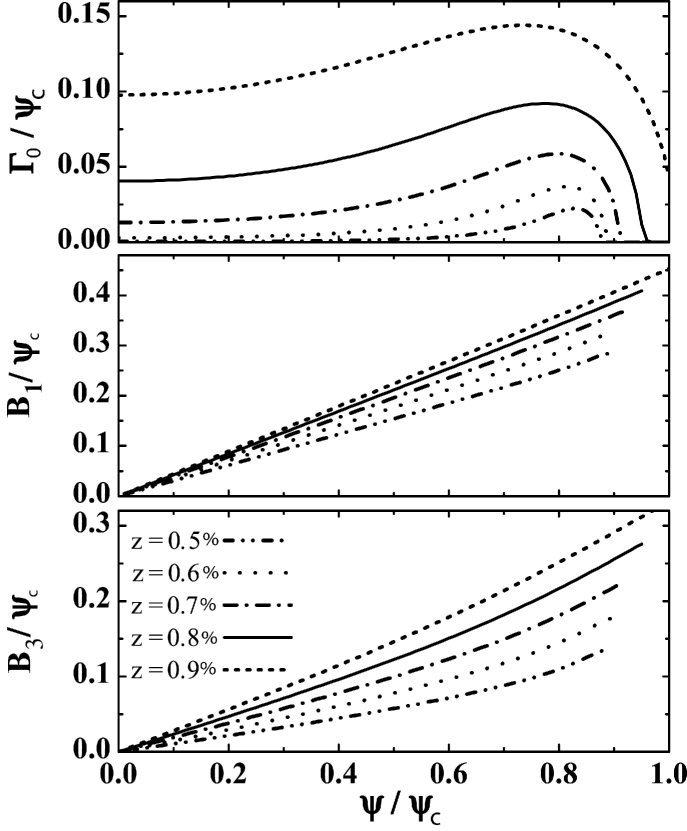
Figure 4: Effect of disorder on charge-order-dependence of self-energy components. To satisfy Dyson’s equation, it is necessary to include three (extended-Nambu space) components of the self energy. Their self-consistent values are plotted here for several different values of impurity fraction $z$. Here, the scattering potential is given in our three parameter model as $\{V_{1},R_{2},R_{3}\}=\{110,0.9,0.8\}$, which represents a fairly short-ranged potential. These results are for the case of isotropic nodes ($v_{f}=v_{\Delta}$). All energies are in units of $\psi_{c}$.

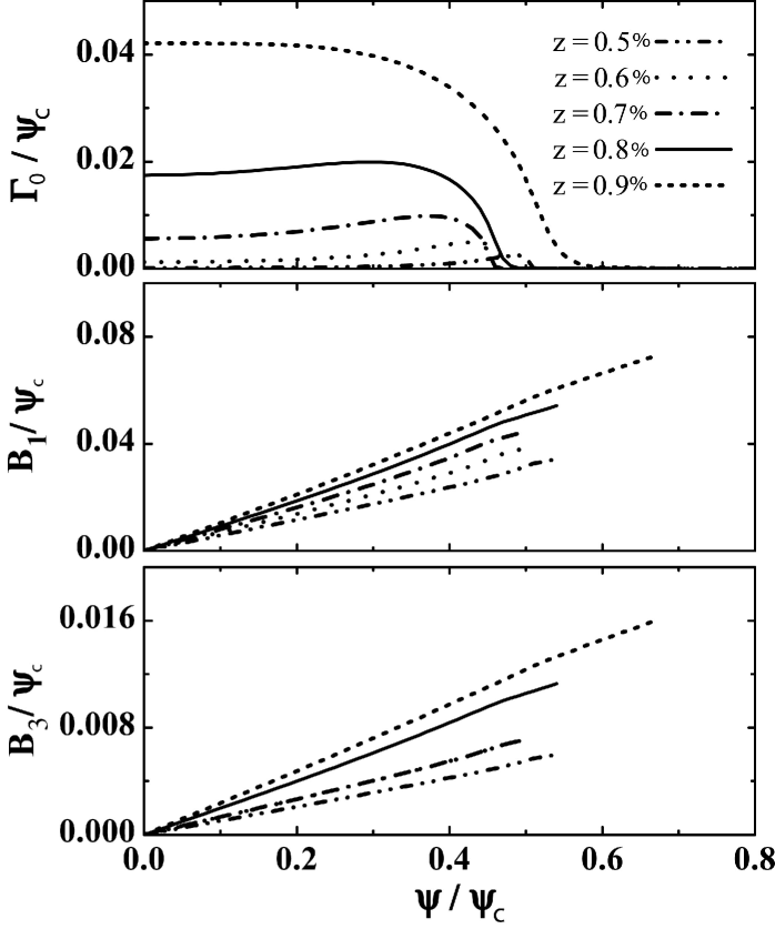
Figure 5: Effect of disorder on charge-order-dependence of self-energy components. This figure illustrates the case where $v_{f}=16v_{\Delta}$. The scattering potential is again given by $\{V_{1},R_{2},R_{3}\}=\{110,0.9,0.8\}$, representing a fairly short-ranged potential. The plots for $B_{1}$ and $B_{3}$ terminate before $\psi$ reaches $\psi_{c}$ because for sufficiently large $\psi$, the excitations become gapped and our nodal approximations break down.

The observed $z$ dependence is not very surprising, in light of Eq. (13). The self-energy components depend on $z$ roughly according to

$$\Gamma_{0} \sim p_{0}\exp{(-\frac{1}{z})}$$

$$B_{1} \sim z$$

$$B_{3} \sim z$$ (18)

as can be seen in Fig. 6. When $\psi=0$, $\Gamma_{0}$ is given by the closed-form expression obtained in Ref. dur01, , $\Gamma_{0}=p_{0}\exp(\frac{-1}{2\pi c})$, where $c=\frac{n_{i}(V_{1}^{2}+2V_{2}^{2}+V_{3}^{2})}{8\pi^{2}v_{f}v_{\Delta}}$. For finite $\psi$, this precise form does not hold, but the strong $z$ dependence of $\Gamma_{0}$ remains, in contrast to that of $B_{1}$ and $B_{3}$. Note that the $z$ dependence of $B_{1}$ and $B_{3}$ is roughly linear for $\psi\ll\psi_{c}^{*}$. As $\psi$ approaches $\psi_{c}^{*}$ the functions diverge slightly from linearity. Results for several values of $\psi<\psi_{c}^{*}$ are shown in the figure.

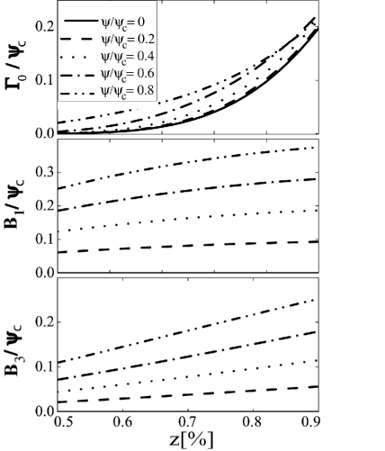
Figure 6: Effect of charge order on disorder-dependence of self-energy components. Nonzero components of $\widetilde{\Sigma}(z)$ are shown for impurity fraction $z$ ranging from $0.5$ to $1.0\%$, for charge order parameter $\psi$=0, 0.2, 0.4, 0.6, and 0.8 (in units of $\psi_{c}$). These results are for scattering parameters $\{V_{1},R_{2},R_{3}\}=\{110,0.9,0.8\}$ and $v_{f}=v_{\Delta}$. Similar results are obtained for the case of anisotropic nodes.

IV Thermal Conductivity

Thermal conductivity was calculated using the Kubo formula mah01 ; Fetter ,

$$\frac{\kappa(\Omega,T)}{T}=-\frac{\mathrm{Im}\Pi_{\mathrm{Ret}}(\Omega)}{\Omega\,\,T^{2}},$$ (19)

where $\Pi_{\mathrm{Ret}}(\Omega)$ is the retarded thermal current-current correlation function. To find this correlator, it is necessary to first compute the appropriate thermal current operator. For our model hamiltonian, this is done in Ref. dur02, with the result

$$\mathbf{\widetilde{j}}^{\kappa}_{0}=\lim_{\begin{subarray}{c}q\rightarrow 0\\ \Omega\rightarrow 0\end{subarray}}\sum_{\begin{subarray}{c}k,\omega\end{subarray}}(\omega+\frac{\Omega}{2})\psi^{\dagger}_{k}\left(\widetilde{\mathbf{v}}_{fM}+\widetilde{\mathbf{v}}_{\Delta M}\right)\psi_{k+q},$$ (20)

where a generalized velocity is defined as

$$\widetilde{\mathbf{v}}_{\alpha M}=v_{\alpha}^{x}\widetilde{M}_{\alpha}^{x}\hat{x}+v_{\alpha}^{y}\widetilde{M}_{\alpha}^{y}\hat{y}$$

$$\widetilde{M}_{\alpha}^{x}\equiv\widetilde{(\sigma_{3}\otimes\tau_{\alpha})}\hskip 15.0pt\widetilde{M}_{\alpha}^{y}\equiv\widetilde{(\sigma_{0}\otimes\tau_{\alpha})}$$ (21)

where $\alpha=\{f,\Delta\}$ and $\tau_{\alpha}=\{\tau_{3},\tau_{1}\}$ for Fermi and gap velocities respectively.

To calculate a thermal conductivity that satisfies Ward identities, vertex corrections must be included on the same footing as the self-energy corrections to the single particle Green’s function. The details of this calculation are similar to those performed in Appendix B of Ref. dur01, . The impurity scattering diagrams which contribute to the ladder series of diagrams are included by expressing the correlation function in terms of a dressed vertex, as shown in Fig. 7.

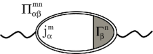
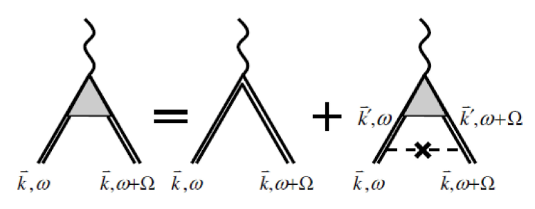
Figure 7: (a) Feynman diagram representing the correlation function $\Pi_{\alpha\beta}^{\mathrm{mn}}$ in terms of a bare vertex $j_{\alpha}^{\mathrm{m}}$, and a dressed vertex $\Gamma_{\beta}^{\mathrm{n}}$. (b) Feynman diagram representing the (ladder series) dressed vertex in terms of the bare vertex and the Born scattering event.

The current-current correlation function is obtained from this dressed bubble. The bare current operator of Eq. (20) is associated with one vertex of the bubble, while the dressed vertex of Fig. 7 is associated with the other. Evaluating Fig. 7, we find that the current-current correlation function takes the form

$$\Pi^{mn}(i\Omega)=\sum_{\alpha,\beta=f,\Delta}\Pi^{mn}_{\alpha\beta}(i\Omega)$$

$$\Pi^{mn}_{\alpha\beta}(i\Omega)=\frac{1}{k_{B}T}\sum_{i\omega}(i\omega+\frac{i\Omega}{2})^{2}\sum_{k}$$

$$\mathrm{Tr}\left[\widetilde{\mathcal{G}_{1}}v_{\alpha}k_{\alpha}^{m}\widetilde{M_{\alpha}^{m}}\widetilde{\mathcal{G}_{2}}v_{\beta}\widetilde{M_{\beta}^{n}}\widetilde{\Gamma_{\beta}^{n}}\right]$$ (22)

where $\widetilde{\mathcal{G}}_{1}\equiv\widetilde{\mathcal{G}(\mathbf{k},i\omega})$, $\widetilde{\mathcal{G}_{2}}\equiv\widetilde{\mathcal{G}}(\mathbf{k},i\omega+i\Omega)$, and $\widetilde{\Gamma_{\beta}^{n}}=\widetilde{\Gamma_{\beta}^{n}}(\mathbf{k},i\omega,i\Omega)$ represents the dressed vertex depicted in Fig. 7. The Greek indices denote “Fermi” and “gap” terms, while the Roman indices denote the position space components of the tensor. We use Fig. 7 to find the form of the vertex equation, and then make the ansatz that

$$\widetilde{\mathbf{\Gamma}_{\beta}}(\mathbf{k},i\omega,i\Omega)=\Big{(}\widetilde{\openone}+\widetilde{\Lambda}(|\mathbf{k}|,i\omega,i\Omega)\Big{)}\hat{k},$$ (23)

which leads to the scalar equations

$$\widetilde{\Gamma}_{\beta}^{n}(\mathbf{k},i\omega,i\Omega)=k_{n}(\widetilde{\openone}+\widetilde{\Lambda}_{\beta}^{n}).$$ (24)

Looking for solutions of this form, we see that the scalar vertex function is

$$\widetilde{\Lambda}_{\beta}^{n}=\mathrm{n}_{i}\sum_{k^{\prime}}\widetilde{M}_{\beta}^{n}\widetilde{V}_{kk^{\prime}}\widetilde{\mathcal{G}}_{2}\widetilde{M}_{\beta}^{n}(\widetilde{\openone}+\widetilde{\Lambda}_{\beta}^{n})\widetilde{\mathcal{G}}_{1}\widetilde{V}_{k^{\prime}k}\frac{k^{{}^{\prime}n}_{\beta}}{k^{n}_{\beta}}.$$ (25)

Since we are working with nodal quasiparticles, we utilize the parametrization of Eq. (II), so that the vertex function is now a function of node index $j$ and local momentum $\mathbf{p}$

$$\widetilde{\Lambda}_{\beta}^{n} = n_{\mathrm{imp}}\sum_{j^{\prime}=1}^{4}\underline{V}_{jj^{\prime}}\underline{V}_{j^{\prime}j}(\frac{k_{\beta n}^{(j^{\prime})}}{k_{\beta n}^{(j)}})\int\frac{\mathrm{d}^{2}p^{\prime}}{8\pi^{2}v_{f}v_{2}}$$ (26)

$$\widetilde{M}_{\beta}^{n}(\widetilde{\sigma_{0}\otimes\tau_{3}})\widetilde{\mathcal{G}}_{2}\widetilde{M}_{\beta}^{n}(\widetilde{\openone}+\widetilde{\Lambda}_{\beta}^{n})\widetilde{\mathcal{G}}_{1}(\widetilde{\sigma_{0}\otimes\tau_{3}}).$$

Arbitrarily choosing $j=1$, then for $j^{\prime}=\{1,2,3,4\}$

$$\frac{k_{1x}^{(j^{\prime})}}{k_{1x}^{(1)}}=\{1,-1,-1,1\}\hskip 20.0pt\frac{k_{1y}^{(j^{\prime})}}{k_{1y}^{(1)}}=\{1,1,-1,-1\}$$

$$\frac{k_{2x}^{(j^{\prime})}}{k_{2x}^{(1)}}=\{1,-1,-1,1\}\hskip 20.0pt\frac{k_{2y}^{(j^{\prime})}}{k_{2y}^{(1)}}=\{1,1,-1,-1\}.$$ (27)

Using the node space matrix representing the 3-parameter scattering potential

$$\underline{V}_{jj^{\prime}}=\begin{pmatrix}V_{1}&V_{2}&V_{3}&V_{2}\\ V_{2}&V_{1}&V_{2}&V_{3}\\ V_{3}&V_{2}&V_{1}&V_{2}\\ V_{2}&V_{3}&V_{2}&V_{1}\end{pmatrix}$$ (28)

we obtain for the vertex equation

$$\widetilde{\Lambda}^{n}_{\beta}=\gamma\int\frac{\mathrm{d}^{2}p^{\prime}}{\pi}\widetilde{M}_{\beta}^{n}(\widetilde{\sigma_{0}\otimes\tau_{3}})\widetilde{\mathcal{G}}_{2}\widetilde{M}_{\beta}^{n}(\widetilde{\openone}+\widetilde{\Lambda}_{\beta}^{n})\widetilde{\mathcal{G}}_{1}(\widetilde{\sigma_{0}\otimes\tau_{3}})$$ (29)

where $\gamma\equiv n_{\mathrm{imp}}\frac{V_{1}^{2}-V_{3}^{2}}{8\pi v_{f}v_{2}}$. The correlator then becomes

$$\Pi_{\alpha\beta}^{mn}(i\Omega) = v_{\alpha}v_{\beta}\frac{1}{\beta}\sum_{i\omega}(i\omega+\frac{i\Omega}{2})^{2}\sum_{k}(k_{\alpha m}k_{\beta n})$$ (30)

$$\mathrm{Tr}\left(\widetilde{\mathcal{G}}_{1}\widetilde{M}_{\alpha}^{m}\widetilde{\mathcal{G}}_{2}\widetilde{M}_{\beta}^{n}(\widetilde{\openone}+\widetilde{\Lambda}_{\beta}^{n})\right)$$

$$= v_{\alpha}v_{\beta}\frac{1}{\beta}\sum_{i\omega}(i\omega+\frac{i\Omega}{2})^{2}\sum_{j=1}^{4}(k_{\alpha m}^{(j)}k_{\beta n}^{(j)})$$

$$\int\frac{\mathrm{d}^{2}p}{8\pi^{2}v_{f}v_{\Delta}}\mathrm{Tr}\left(\widetilde{\mathcal{G}}_{1}\widetilde{M}_{\alpha}^{m}\widetilde{\mathcal{G}}_{2}\widetilde{M}_{\beta}^{n}(\widetilde{\openone}+\widetilde{\Lambda}_{\beta}^{n})\right).$$

Since

$$\sum_{j=1}^{4}k_{\alpha m}^{(j)}k_{\beta n}^{(j)}=2\left((1-\delta_{\alpha\beta})\eta_{m}+\delta_{\alpha\beta}\right)\delta_{mn}$$ (31)

we can write

$$\Pi_{\alpha\beta}^{mn}(i\Omega)=2\pi c_{\alpha\beta}^{mn}\frac{1}{\beta}\sum_{i\omega}(i\omega+\frac{i\Omega}{2})^{2}\mathrm{Tr}\left(\widetilde{I}_{\alpha\beta}^{mn}(\widetilde{\openone}+\widetilde{\Lambda}_{\beta}^{n})\right)$$ (32)

where

$$c_{\alpha\beta}^{mn} \equiv \frac{1}{8\pi^{2}}\frac{v_{\alpha}v_{\beta}}{v_{f}v_{\Delta}}\Big{(}(1-\delta_{\alpha\beta})\eta_{m}+\delta_{\alpha\beta}\Big{)}\delta_{mn}$$ (33)

and

$$\widetilde{I}_{\alpha\beta}^{mn}(i\omega,i\omega+i\Omega) \equiv \int\frac{\mathrm{d}^{2}p}{\pi}\widetilde{\mathcal{G}}_{1}\widetilde{M}_{\alpha}^{m}\widetilde{\mathcal{G}}_{2}\widetilde{M}_{\beta}^{n}.$$ (34)

To calculate the conductivity, we will need Tr$(\widetilde{I}_{\alpha\beta}^{m})$ and Tr$(\widetilde{I}_{\alpha\beta}^{m}\widetilde{\Lambda}_{\beta}^{n})$. For $\psi=0$, it is possible to compute the integral in Eq. (34) analytically, but for general $\psi$ we had to compute the integrals numerically. We note that if we write

$$\widetilde{I}=\begin{pmatrix}I_{A}&I_{B}\\ I_{C}&I_{D}\end{pmatrix},$$ (35)

apply the symmetry properties of Eq. (14) and reverse the order of integration of $p_{1}$ and $p_{2}$, then $I_{A}=I_{D}$, and $I_{B}=I_{C}$, so that the most general expansion of $\widetilde{I}_{\alpha\beta}^{mn}$ in Nambu space is

$$\widetilde{I}_{\alpha\beta}^{mn}=\sum_{i=0}^{1}\sum_{i^{\prime}=0}^{3}(I_{\alpha\beta}^{mn})_{ii^{\prime}}(\widetilde{\sigma_{i}}\otimes\tau_{i^{\prime}}).$$ (36)

Then

$$\mathrm{Tr}(\widetilde{I}_{\alpha\beta}^{mn}) = \mathrm{Tr}\left(\sum_{i=0}^{1}\sum_{i^{\prime}=0}^{3}(I_{\alpha\beta}^{mn})_{ii^{\prime}}(\widetilde{\sigma_{i}\otimes\tau_{i^{\prime}}})\right)$$ (37)

$$= 4(I_{\alpha\beta}^{mn})_{00},$$

while if we use the same expansion for

$$\widetilde{\Lambda}_{\beta}^{n}=\sum_{i=0}^{1}\sum_{i^{\prime}=0}^{3}(\Lambda_{\beta}^{n})_{ii^{\prime}}(\widetilde{\sigma_{i}\otimes\tau_{i^{\prime}}}),$$ (38)

we find

$$\mathrm{Tr}(\widetilde{I}_{\alpha\beta}^{mn}\widetilde{\Lambda}_{\beta}^{n})=\sum_{ij=0}^{1}\sum_{i^{\prime}j^{\prime}=0}^{3}(I_{\alpha\beta}^{mn})_{ii^{\prime}}(\Lambda_{\beta}^{n})_{jj^{\prime}}$$

$$\mathrm{Tr}(\widetilde{\sigma_{i}\sigma_{j}\otimes\tau_{i^{\prime}}\tau_{j^{\prime}}})$$

$$=4\sum_{i=0}^{1}\sum_{i^{\prime}=0}^{3}(I_{\alpha\beta}^{mn})_{ii^{\prime}}(\Lambda_{\beta}^{n})_{ii^{\prime}}.$$ (39)

Then Eq. (29) becomes

$$4(\Lambda_{\beta}^{n})_{ii^{\prime}}=\mathrm{Tr}\left((\widetilde{\sigma_{i}\otimes\tau_{i^{\prime}}})\widetilde{\Lambda}_{\beta}^{n}\right)$$

$$=\gamma\int\frac{\mathrm{d}^{2}p}{\pi}\mathrm{Tr}((\widetilde{\sigma_{i}\otimes\tau_{i^{\prime}}})\widetilde{M}_{\beta}^{n}(\widetilde{\sigma_{0}\otimes\tau_{3}})$$ (40)

$$\widetilde{\mathcal{G}}_{2}\widetilde{M}_{\beta}^{n}(\widetilde{\openone}+\widetilde{\Lambda_{\beta}^{n}})\widetilde{\mathcal{G}}_{1}(\widetilde{\sigma_{0}\otimes\tau_{3}}))$$

$$=\gamma\mathrm{Tr}\left(\widetilde{L}_{\beta ii^{\prime}}^{n}(\widetilde{1}+\widetilde{\Lambda}_{\beta}^{n})\right)$$ (41)

where

$$\widetilde{L}_{\beta ii^{\prime}}^{n}\equiv\int\frac{\mathrm{d}^{2}p}{\pi}\widetilde{\mathcal{G}}_{1}(\widetilde{\sigma_{0}\otimes\tau_{3}})(\widetilde{\sigma_{i}\otimes\tau_{i^{\prime}}})$$

$$\widetilde{M}_{\beta}^{n}(\widetilde{\sigma_{0}\otimes\tau_{3}})\widetilde{\mathcal{G}}_{2}\widetilde{M}_{\beta}^{n}.$$ (42)

The symmetries of $\widetilde{\mathcal{G}}$ which were used to see which components of $\widetilde{I}_{\alpha\beta}^{mn}$ were $0$ can also be applied to $\widetilde{L}_{\beta ii^{\prime}}^{n}$ with the result that $(L_{\beta ii^{\prime}}^{n})_{A}=(L_{\beta ii^{\prime}}^{n})_{D}$, $(L_{\beta ii^{\prime}}^{n})_{B}=\eta_{i}(L_{\beta ii^{\prime}}^{n})_{C}$, where $\eta_{i}=\left\{\begin{array}[]{c}+1,\,i=0,1\\ -1,\,i=2,3\end{array}\right\}$. Since all that is required for the conductivity is $i=0,1$, we use the expansion

$$\widetilde{L}_{\beta ii^{\prime}}^{n}=\sum_{j=0}^{1}\sum_{j^{\prime}=0}^{3}(\widetilde{\sigma_{j}\otimes\tau_{j^{\prime}}})(L_{\beta ii^{\prime}}^{n})_{jj^{\prime}}$$ (43)

so that

$$(\Lambda_{\beta}^{n})_{ii^{\prime}}=\frac{1}{4}\gamma\mathrm{Tr}\left(\widetilde{L}_{\beta ii^{\prime}}^{n}(\widetilde{\openone}+\widetilde{\Lambda}_{\beta}^{n})\right)$$

$$=\frac{1}{4}\gamma\,\,\mathrm{Tr}\,(\sum_{j=0}^{1}\sum_{j^{\prime}=0}^{3}(L_{\beta ii^{\prime}}^{n})_{jj^{\prime}}(\widetilde{\sigma_{j}\otimes\tau_{j^{\prime}}})$$

$$+\sum_{jk=0}^{1}\sum_{j^{\prime}k^{\prime}=0}^{3}(L_{\beta ii^{\prime}})_{jj^{\prime}}(\Lambda_{\beta}^{n})_{kk^{\prime}})$$

$$=\gamma\left((L_{\beta ii^{\prime}}^{n})_{00}+\sum_{j=0}^{1}\sum_{j^{\prime}=0}^{3}(L_{\beta ii^{\prime}}^{n})_{jj^{\prime}}(\Lambda_{\beta}^{n})_{jj^{\prime}}\right).$$ (44)

The thermal conductivity is obtained from the retarded current-current correlation function

$$\frac{\kappa^{mn}(\Omega)}{T}=-\frac{1}{T}\frac{\mathrm{Im}\left(\Pi_{\mathrm{ret}}^{mn}(\Omega)\right)}{\Omega},$$ (45)

where $\Pi_{\mathrm{ret}}(\Omega)=\Pi(i\Omega\rightarrow\Omega+i\delta).$ To get the retarded correlator we first perform the Matsubara summation. Consider the summand of Eq. 32, which we redefine according to

$$J(i\omega,i\omega+i\Omega)=\mathrm{Tr}\left(\widetilde{I}_{\alpha\beta}^{mn}(\widetilde{\openone}+\widetilde{\Lambda}_{\beta}^{n})\right).$$ (46)

The function $J(i\omega,i\omega+i\Omega)$ is of the form $J(i\omega,i\omega+i\Omega)=f(A(i\omega)B(i\omega+i\Omega))$ where $A$ and $B$ are dressed Green’s functions of a complex variable $z=i\omega_{n}$, so that $J$ is analytic with branch cuts occurring where $z$ and $z+i\Omega$ are real. The Matsubara summation needed is performed by integrating on a circular path of infinite radius, so that the only contribution is from just above and just below the branch cuts,

$$\Pi_{\alpha\beta}^{mn}=-c_{\alpha\beta}^{mn}\frac{1}{i}\oint\mathrm{d}z(z+\frac{i\Omega}{2})^{2}J(z,z+i\Omega)$$

$$=-c_{\alpha\beta}^{mn}\frac{1}{i}\int_{-\infty}^{\infty}\mathrm{d}\epsilon\,n_{f}(\epsilon)\Big{(}$$

$$(\epsilon+\frac{i\Omega}{2})^{2}(J(\epsilon+i\delta,\epsilon+i\Omega)-J(\epsilon-i\delta,\epsilon+i\Omega))$$

$$+(\epsilon-\frac{i\Omega}{2})^{2}(J(\epsilon-i\Omega,\epsilon+i\delta)-J(\epsilon-i\Omega,\epsilon-i\delta))\Big{)}.$$ (47)

To obtain the retarded function, we analytically continue $i\Omega\rightarrow\Omega+i\delta$. Then we let $\epsilon\rightarrow\epsilon+\Omega$ in the third and fourth terms, so that

$$\Pi_{\alpha\beta}^{mn}(\Omega)_{\mathrm{ret}} = c_{\alpha\beta}^{mn}\int_{-\infty}^{\infty}\mathrm{d}\epsilon\,n_{f}(\epsilon+\Omega)-n_{f}(\epsilon))(\epsilon+\frac{\Omega}{2})^{2}$$ (48)

$$\times\mathrm{Re}\Big{(}J_{\alpha\beta}^{AR}(\epsilon,\epsilon+\Omega)-J_{\alpha\beta}^{RR}(\epsilon,\epsilon+\Omega)\Big{)}$$

where $J^{AR}$ and $J^{RR}$ are defined by Eqs. (46) and (IV) and are composed of the universal-limit Green’s functions given in Appendix A. Taking the imaginary part, we find

$$\frac{\kappa^{mn}(\Omega,T)}{T} = -\int_{-\infty}^{\infty}\mathrm{d}\epsilon\frac{n_{f}(\epsilon+\Omega)-n_{f}(\epsilon)}{\Omega}\left(\frac{\epsilon+\frac{\Omega}{2}}{T}\right)^{2}$$

$$\sum_{\alpha\beta}c_{\alpha\beta}^{mn} \mathrm{Re} (J_{\alpha\beta}^{AR}(\epsilon,\epsilon+\Omega))-J_{\alpha\beta}^{RR}(\epsilon,\epsilon+\Omega)).$$ (49)

In taking the $\Omega\rightarrow 0$ limit, the difference in Fermi functions becomes a derivative. Evaluating the integral, $\int\mathrm{d}\epsilon(-\frac{\mathrm{d}n}{\mathrm{d}\epsilon})(\frac{\epsilon}{T})^{2}=\frac{\pi^{2}k_{B}^{2}}{3}$, we find that

$$\frac{\kappa_{\alpha\beta}^{mm}(0,0)}{T}=\frac{\pi^{2}k_{B}^{2}}{3}c_{\alpha\beta}^{mm}\mathrm{Re}\left(J_{\alpha\beta}^{AR}(0,0)-J_{\alpha\beta}^{RR}(0,0)\right).$$ (50)

That $\kappa^{xy}=\kappa^{yx}=0$ is seen from Eq. (33). Finally, since the $\alpha\neq\beta$ integrals are traceless, the result for the thermal conductivity is

$$\frac{\kappa^{mm}}{T}=\frac{k_{B}^{2}}{3}\frac{v_{f}^{2}+v_{\Delta}^{2}}{v_{f}v_{\Delta}}\frac{1}{8}\left(J_{\alpha\beta}^{AR}(0,0)-J_{\alpha\beta}^{RR}(0,0)\right).$$ (51)

V Results

For a discussion of the units employed in the analysis, one can refer to Sec. III.2. The reduced set of parameters for the model is $\{z,V_{1},R_{2},R_{3},\beta,p_{0},\psi\}$. We explored a limited region of this parameter space, calculating the integrals and solving the matrix equation numerically. In particular, we looked at the $\psi$ dependence of $\kappa$. To vary the anisotropy of the scattering potential, we considered the $\{R_{2},R_{3}\}$ values of $\{0.9,0.8\}$, $\{0.7,0.6\}$, and $\{0.5,0.3\}$, and kept fixed the constant $c$ (given after Eq. (13))by appropriately modifying $V_{1}$. For $\{R_{2},R_{3}\}=\{0.9,0.8\}$, we used $V_{1}=110$. The rationale for keeping $c$ fixed is that the self-energy depends only on $c$, $\beta$ and $p_{0}$. Additionally, we explored the dependence of the thermal conductivity on impurity fraction $z$ and velocity anisotropy $\beta$. For all computations we set the cutoff $p_{0}=100$; this simply fixes a particular value of the product $v_{f}v_{\Delta}$ for these calculations.

V.1 Vertex Corrections

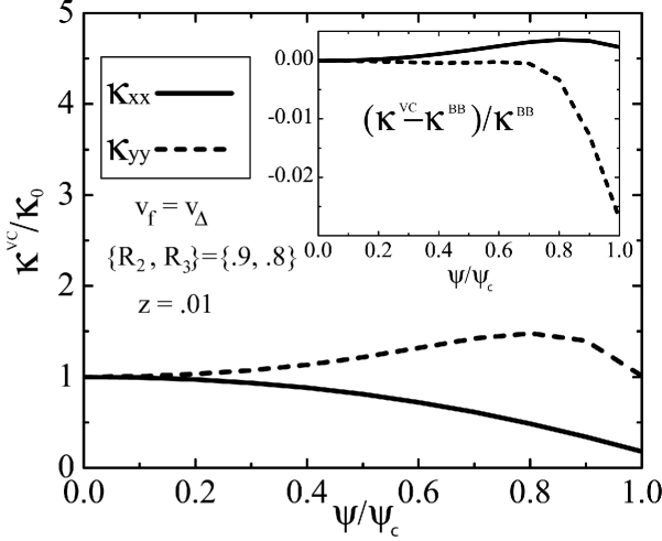
Figure 8: Vertex-corrected thermal conductivity, in units of the universal conductivity $\kappa_{0}/T\equiv\frac{k_{B}}{3\hbar}(v_{f}/v_{\Delta}+v_{\Delta}/v_{f})$. This data reflects a short range scattering potential $\{V_{1},R_{2},R_{3}\}=\{110,0.9,0.8\}$, impurity fraction $z$=0.01, and isotropic Dirac quasiparticles ($v_{f}=v_{\Delta}$). The inset displays the discrepancy between the bare-bubble and vertex-corrected results, in units of the bare-bubble result. It is clear that the vertex corrections are of little quantitative importance for these particular parameters.

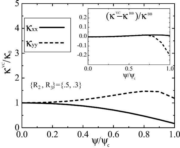
Figure 9: Vertex-corrected thermal conductivity, in units of the universal conductivity $\kappa_{0}/T\equiv\frac{k_{B}}{3\hbar}(v_{f}/v_{\Delta}+v_{\Delta}/v_{f})$. This figure portrays the effect that a different scattering potential has on the importance of vertex corrections. Here, a longer range potential $\{V_{1},R_{2},R_{3}\}=\{140,0.5,0.3\}$ was used, again with impurity fraction $z$=$0.01$ and $v_{f}=v_{\Delta}$. The inset displays the discrepancy between the bare-bubble and vertex-corrected results, in units of the bare-bubble result. From this, we determine that vertex corrections make a more substantial correction as the forward scattering limit is approached, but only once the charge ordering is quite strong.

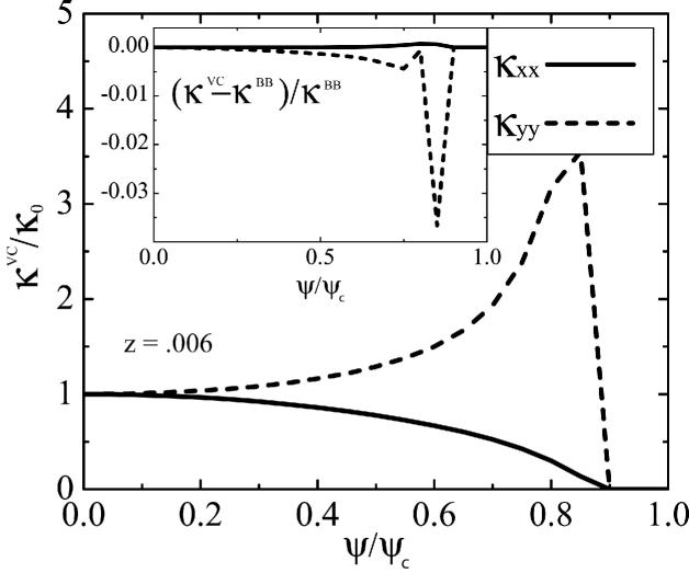
Figure 10: Vertex-corrected thermal conductivity, in units of the universal conductivity $\kappa_{0}/T\equiv\frac{k_{B}}{3\hbar}(v_{f}/v_{\Delta}+v_{\Delta}/v_{f})$. Again, a short-ranged scattering potential, $\{V_{1},R_{2},R_{3}\}=\{110,0.9,0.8\}$ and isotropic nodes ($v_{f}=v_{\Delta}$) are used. This figure displays the effect of a smaller impurity fraction than that depicted in Fig.8. The inset displays the discrepancy between the bare-bubble and vertex-corrected results, in units of the bare-bubble result; since the scattering potential falls off slowly (in k-space) here, the vertex corrections are again quite unimportant.

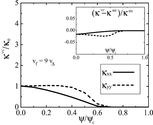
Figure 11: Vertex-corrected thermal conductivity, in units of the universal conductivity $\kappa_{0}/T\equiv\frac{k_{B}}{3\hbar}(v_{f}/v_{\Delta}+v_{\Delta}/v_{f})$, for short-ranged scattering potential, $\{V_{1},R_{2},R_{3}\}=\{110,0.9,0.8\}$ and impurity fraction $z=0.01$. These calculations differ from those of Fig.8 in that they apply to the case of a more anisotropic Dirac spectrum with $v_{f}=9v_{\Delta}$. The thermal conductivity has a qualitatively similar $\psi$ dependence, but vanishes for a smaller value of $\psi$ than for the isotropic case. The inset displays the discrepancy between the bare-bubble and vertex-corrected results, in units of the bare-bubble result; again, the vertex corrections do not significantly modify the bare-bubble results.

The importance of including the vertex corrections is determined by comparing the vertex corrected thermal conductivity with that of the bare-bubble. If $\frac{\kappa^{VC}-\kappa^{BB}}{\kappa^{BB}}<<1$ for a region of parameter space, then in that regime the bare-bubble results can be used instead. This is of threefold practicality: the bare-bubble results are less computationally expensive, the bare-bubble expression is much simpler to analyze, and other hamiltonians could be more easily studied.

The bare bubble thermal conductivity can be obtained by setting $\widetilde{\Lambda}_{\beta}^{n}\rightarrow\widetilde{0}$ in Eq. (46), or by using a spectral representation, as in Ref dur02, ; both methods have the same result. For impurity fraction $z$ ranging from 0.5$\%$ to $1\%$, the importance of the vertex corrections is largely seen to be negligible, which implies that an analysis of the bare bubble results is sufficient.

Figs. 8-11 illustrate the vertex corrected thermal conductivities, $\kappa^{VC}$, in the main graphs, while the insets display the relative discrepancy with respect to the bare bubble thermal conductivities $\frac{\kappa^{VC}-\kappa^{BB}}{\kappa^{BB}}$. Each is plotted as a function of the amplitude of the CDW, $\psi/\psi_{c}$, where $\psi_{c}$ indicates the maximal CDW for which the clean system remains gapless. We will postpone analysis of the character of the thermal conductivity until Sec. V C.

To gauge the importance of the vertex corrections, we look first at Fig. 8. The inset indicates that the vertex corrections do not signifigantly modify the bare bubble thermal conductivity. Although their importance grows somewhat with increasing $\psi$, the correction is still slight.

Next, Fig. 8 is used as a reference against which to consider the dependence of vertex corrections on scattering potential, impurity fraction, and velocity anisotropy. The next three figures are the results of computations with each of these parameters modified in turn. By comparing Fig. 9 with Fig. 8 we conclude that the vertex corrections become more important when the scattering potential is peaked in $k$-space, but are unimportant for potentials that fall off slowly in $k$-space.

Fig. 8 and Fig. 10 correspond roughly to the largest and smallest $z$ for which these calculations are valid. Comparison of these two figures, as well as that of intermediary values of $z$ (not displayed) indicates that the relative importance of the vertex corrections is independent of $z$. Nor does increasing the velocity anisotropy affect their importance, as seen by making a comparison between Fig. 8 and Fig. 11.

V.2 Clean Limit Analysis

It is of great interest to consider the behavior of the thermal conductivity in the clean $(z\rightarrow 0)$ limit. Because the thermal conductivity is composed of integrals over $\mathbf{p}$-space of functions which become increasingly peaked in this limit, there exists a sufficiently small $z$ beyond which it is not possible to perform the requisite numerical integrations. However, it is still possible to obtain information about this regime. To that end, we will examine the form of the bare-bubble thermal conductivity, and consider the $z\rightarrow 0$ limit. As we shall see, this will enable us to determine the value of $\psi$ at which the nodal approximation, and hence this calculation, is no longer valid. Additionally, a closed-form result for the thermal conductivity in the $z\rightarrow 0$ limit is obtained for the isotropic ($v_{f}=v_{\Delta}$) case. The bare-bubble thermal conductivity, identical with setting $\widetilde{\Lambda}\rightarrow\widetilde{0}$ in Eq. (51), is

$$\kappa^{mm} = \frac{k_{B}}{3}\frac{v_{f}^{2}+v_{2}^{2}}{v_{f}v_{2}}J^{m}\hskip 50.0ptJ^{m}=\int\frac{\mathrm{d}^{2}\mathbf{p}}{2\pi}\frac{N_{1}+N_{2}}{D}\hskip 50.0pt\epsilon_{1}\equiv\epsilon_{k}\hskip 50.0pt\Delta_{1}\equiv\Delta_{k}$$

$$N_{1} = A\left((A+B+\epsilon_{1}^{2}+\Delta_{1}^{2})^{2}+(A+B+\epsilon_{2}^{2}+\Delta_{2}^{2})^{2}\right)\hskip 41.0pt\epsilon_{2}\equiv\epsilon_{k+G}\hskip 38.0pt\Delta_{2}\equiv\Delta_{k+G}$$

$$N_{2} = \eta_{m}A\Big{(}(\psi-B_{3})^{2}((\epsilon_{1}+\epsilon_{2})^{2}-(\Delta_{1}-\Delta_{2})^{2})+B_{1}^{2}((\Delta_{1}+\Delta_{2})^{2}-(\epsilon_{1}-\epsilon_{2})^{2})-4B_{1}(\psi-B_{3})(\epsilon_{1}\Delta_{1}+\epsilon_{2}\Delta_{2}))\Big{)}$$

$$D = \Big{[}(A+B+\epsilon_{1}^{2}+\Delta_{1}^{2})(A+B+\epsilon_{2}^{2}+\Delta_{2}^{2})-B\Big{(}(\epsilon_{1}+\epsilon_{2})^{2}+(\Delta_{1}-\Delta_{2})^{2}\Big{)}$$ (52)

$$+4B_{1}\Big{(}B_{1}(\epsilon_{1}\epsilon_{2}-\Delta_{1}\Delta_{2})+(\psi-B_{3})(\epsilon_{1}\Delta_{2}+\epsilon_{2}\Delta_{1})\Big{)}\Big{]}^{2},$$

where $A\equiv\Gamma_{0}^{2}$ and $B\equiv(\psi-B_{3})^{2}+B_{1}^{2}$. Since the results of Section III.2 indicated that $\Gamma_{0}\sim\exp{(-\frac{1}{z})}$ and $B_{1},B_{3}\sim z$, in the $z\rightarrow 0$ limit, $A\rightarrow 0$ much faster than $B_{1}\rightarrow 0$ or $B_{3}\rightarrow 0$. Therefore in taking the $z\rightarrow 0$ limit we will first let $A\rightarrow 0$ to obtain a result still expressed in terms of $B_{1}$ and $B_{3}$. The denominator can be rearranged as

$$D = \Big{(}(A^{2}+A(2B+\epsilon_{1}^{2}+\Delta_{1}^{2}+\epsilon_{2}^{2}+\Delta_{2}^{2})+f\Big{)}^{2}\hskip 20.0pt\mathrm{where}$$

$$f = B^{2}+(\epsilon_{1}^{2}+\Delta_{1}^{2})(\epsilon_{2}^{2}+\Delta_{2}^{2})-2B(\epsilon_{1}\epsilon_{2}-\Delta_{1}\Delta_{2})+4\Big{(}B_{1}(\epsilon_{1}\epsilon_{2}-\Delta_{1}\Delta_{2})+(\psi-B_{3})(\epsilon_{1}\Delta_{2}+\epsilon_{2}\Delta_{1})\Big{)}$$ (53)

$$= \Big{(}(\epsilon_{1}\epsilon_{2}-\Delta_{1}\Delta_{2})-(2B_{1}^{2}-B)\Big{)}^{2}+\Big{(}(\epsilon_{1}\Delta_{2}+\epsilon_{2}\Delta_{1})+2B_{1}(\psi-B_{3})\Big{)}^{2}$$

We are thus considering, in the limit that $A\rightarrow 0$, an integral of the form

$$\int\mathrm{d}^{2}\mathbf{p}\frac{A\,g(\mathbf{p})}{\big{(}Ah(\mathbf{p})+f(\mathbf{p})\big{)}^{2}}$$ (54)

Note that any nonzero contribution to this integral must come from a region in $\mathbf{p}$-space in which $f(\mathbf{p})=0$. We will consider separately the isotropic case ($v_{f}=v_{\Delta}$) and the anisotropic case ($v_{f}>v_{\Delta}$).

V.2.1 Isotropic Case

For the special case where $v_{f}=v_{\Delta}$, it is possible to calculate the integral of Eq. (V.2) exactly, by taking the $A\rightarrow 0$ limit, and choosing another parametrization. The coordinates $q_{1}\equiv\epsilon_{k}-\epsilon_{k+Q}$ and $q_{2}\equiv\epsilon_{k}+\epsilon_{k+Q}-1$, have their origin located at the midpoint of the white and gray dots of Fig. 1. Using these coordinates, in the $A\rightarrow 0$ limit we find that the elements of Eq. (V.2) become

$$N_{1} = 2A\Big{(}B^{2}+B(q^{2}+1)+\frac{1}{4}(q^{2}+1)^{2}+q^{2}-q_{2}^{2}\Big{)}$$

$$N_{2} = 2\eta_{m}A\Big{(}(\psi-B_{3})^{2}((\epsilon_{1}+\epsilon_{2})^{2}-(\Delta_{1}-\Delta_{2})^{2})+B_{1}^{2}((\Delta_{1}+\Delta_{2})^{2}-(\epsilon_{1}-\epsilon_{2})^{2})-4B_{1}(\psi-B_{3})(\epsilon_{1}\Delta_{2}+\epsilon_{2}\Delta_{1})\Big{)}$$

$$= 2\eta_{m}\Big{(}(\psi-B_{3})^{2}(q_{2}^{2}+2q_{2}+1-q_{1}^{2})+B_{1}^{2}(q_{2}^{2}-2q_{2}+1-q_{1}^{2})-4B_{1}(\psi-B_{3})(2q_{2}^{2}-q^{2}-1)\Big{)}$$

$$= 2\eta_{m}A\Big{[}(2q_{2}^{2}-q^{2}+1)\Big{(}(\psi-B_{3})^{2}-2B_{1}(\psi-B_{3})+B_{1}^{2}\Big{)}+2q_{2}\Big{(}(\psi-B_{3})^{2}-B_{1}^{2}\Big{)}+4B_{1}(\psi-B_{3})\Big{]}$$

$$D = \Big{[}2A\Big{(}1+B-2B_{1}(\psi-B_{3})\Big{)}+\Big{(}q_{2}-(\psi^{2}-B_{1}^{2})^{2}\Big{)}^{2}+\frac{1}{4}\Big{(}q^{2}-(1-4B_{1}(\psi-B_{3}))\Big{)}^{2}\Big{]}^{2}.$$ (55)

Now the part of the denominator not proportional to $A$, the $f$-term, is zero when

$$q_{2}=(\psi-B_{3})^{2}-B_{1}^{2}\hskip 10.0pt\mathrm{and}\hskip 10.0ptq^{2}=1-4B_{1}(\psi-B_{3}).$$ (56)

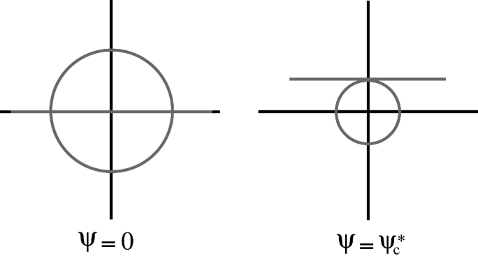
Figure 12: Illustrated is a schematic view of the line and circle whose intersection determines whether gapless excitations remain, for the isotropic case ($v_{f}=v_{\Delta}$). The left figure indicates the situation in the absence of charge ordering, that is, for $\psi=0$, where the radius of the circle is 1 and the line lies on the horizontal axis. The right figure indicates the situation at $\psi=\psi_{c}^{*}$, when charge ordering is such that the excitation spectrum becomes gapped. In the clean case, the $\psi$ evolution corresponds to moving the line past the circle. With self-consistent disorder, the radius of the circle and height of the line are both functions of $\psi$; in each instance, this construction can be used to determine the value of $\psi$ at which the quasiparticle spectrum becomes gapped. This value of $\psi$ is referred to as $\psi_{c}^{*}$ in this paper.

In $q_{1}/q_{2}$ coordinates, these are the equations of a horizontal line and a circle, which must intersect for there to be a nonzero contribution to the integral, since each term is positive definite. In the simplified disorder treatment of Ref. dur02, for which $B_{1}=B_{3}=0$ and $\Gamma_{0}=\mathrm{constant}$, these constraints simplify to $q_{2}=\psi^{2}$ and $q^{2}=1$, so that no contribution occurs when $\psi>1$ (Note that as in the numerical analysis, $\psi$, being an energy, is measured in units of $\psi_{c}$). With the self-consistent treatment of disorder, there will likewise be a sufficiently large value of $\psi$ beyond which the line and circle no longer intersect; we will call this value $\psi_{c}^{*}$ (see Fig. 12). We interpret $\psi_{c}^{*}$ as the point beyond which the system becomes effectively gapped. This is consistent with the exact result found by computing the eigenvalues of the completely clean hamiltonian (as $\psi_{c}^{*}=\psi_{c}$ in that case).

In Sec. III.2 it was determined that $B_{1}\simeq b_{1}\psi$ and $B_{3}\simeq b_{3}\psi$, where $b_{1}$ and $b_{3}$ depend on the remaining parameters of the model. Using this approximate form for $B_{1}$ and $B_{3}$, the condition for the maximum $\psi$ for which the constraints of Eq. (56) are satisfied,

$$1-4B_{1}(\psi-B_{3})=\Big{(}(\psi-B_{3})^{2}-B_{1}^{2}\Big{)}^{2},$$ (57)

indicates that

$$\psi_{c}^{*2}\simeq\frac{\pm\Big{(}(1-b_{3})\mp b_{1}\Big{)}^{2}}{\Big{(}(1-b_{3}-b_{1})(1-b_{3}+b_{1})\Big{)}^{2}}.$$ (58)

Since $\psi_{c}^{*2}>0$, we find that for $v_{f}=v_{\Delta}$,

$$\psi_{c}^{*}\simeq\frac{1}{1-b_{3}+b_{1}}.$$ (59)

We now proceed with the calculation of the clean-limit thermal conductivity. Substituting the conditions of Eq. (56) into Eq. (V.2.1), we find that the numerators become

$$N_{1} = 4A\Big{[}\Big{(}1-2B_{1}(\psi-B_{3})\Big{)}\Big{(}1+B-2B_{1}(\psi-B_{3})\Big{)}\Big{]}$$

$$N_{2} = 4\eta_{m}A\Big{(}1+B-2B_{1}(\psi-B_{3})\Big{)}\Big{(}[(\psi-B_{3})^{2}-B_{1}^{2}]^{2}+2B_{1}(\psi-B_{3})\Big{)}$$ (60)

both of which are independent of $\mathbf{q}$, so that the clean limit result hinges upon the integral

$$I=\int\frac{\mathrm{d}^{2}q}{4\pi}\frac{A}{\Big{(}k_{1}A+(q_{2}-k_{2})^{2}+\frac{1}{4}(q^{2}-k_{3})^{2}\Big{)}^{2}},$$ (61)

where

$$k_{1} = 2\Big{(}1+B-2B_{1}(\psi-B_{3})\Big{)}$$

$$k_{2} = (\psi-B_{3})^{2}-B_{1}^{2}$$

$$k_{3} = 1-4B_{1}(\psi-B_{3}).$$ (62)

The details of this integration are reported in Appendix C, with the result

$$I=\frac{1}{2k_{1}\sqrt{k_{3}-k_{1}^{2}}}.$$ (63)

We can now write the anisotropic clean limit thermal conductivity

$$J = \frac{1-2B_{1}\psi+\eta_{m}\Big{(}[(\psi-B_{3})^{2}-B_{1}^{2}]^{2}+2B_{1}(\psi-B_{3})\Big{)}}{\sqrt{1-4B_{1}(\psi-B_{3})-[(\psi-B_{3})^{2}-B_{1}^{2}]^{2}}}\hskip 3.0pt\Theta\Big{(}1-4B_{1}(\psi-B_{3})-[(\psi-B_{3})^{2}-B_{1}^{2}]^{2}\Big{)}$$

$$J^{xx} = \sqrt{1-4B_{1}(\psi-B_{3})-[(\psi-B_{3})^{2}-B_{1}^{2}]^{2}}\hskip 6.0pt\Theta\Big{(}1-4B_{1}(\psi-B_{3})-[(\psi-B_{3})^{2}-B_{1}^{2}]^{2}\Big{)}$$

$$J^{yy} = \frac{1+[(\psi-B_{3})^{2}-B_{1}^{2}]^{2}}{\sqrt{1-4B_{1}(\psi-B_{3})-[(\psi-B_{3})^{2}-B_{1}^{2}]^{2}}}\hskip 6.0pt\Theta\Big{(}1-4B_{1}(\psi-B_{3})-[(\psi-B_{3})^{2}-B_{1}^{2}]^{2}\Big{)},$$ (64)

where the $\Theta$ function is the Heaviside step function. Using the definition for $\psi_{c}^{*}$ found in Eq. (59), and defining

$$\chi\equiv\frac{1}{1-b_{3}-b_{1}},$$ (65)

we are able to rewrite the dimensionless conductivity in terms of parameters easily extrapolated from SCBA calculations

$$J^{xx} = \frac{\kappa^{xx}}{\kappa_{0}}=\sqrt{\Big{(}1-\frac{\psi^{2}}{\psi_{c}^{*2}}\Big{)}\Big{(}1+\frac{\psi^{2}}{\chi^{2}}\Big{)}}\hskip 5.0pt\Theta[\Big{(}1-\frac{\psi^{2}}{\psi_{c}^{*2}}\Big{)}]$$

$$J^{yy} = \frac{\kappa^{yy}}{\kappa_{0}}=\Big{(}1+\frac{\psi^{4}}{\psi_{c}^{*2}\chi^{2}}\Big{)}\Big{(}1-\frac{\psi^{2}}{\psi_{c}^{*2}}\Big{)}^{-1/2}\Big{(}1+\frac{\psi^{2}}{\chi^{2}}\Big{)}^{-1/2}\hskip 6.0pt\Theta[\Big{(}1-\frac{\psi^{2}}{\psi_{c}^{*2}}\Big{)}]$$ (66)

in which form it is clear that the thermal conductivity vanishes for $\psi>\psi_{c}^{*}$.

V.2.2 Anisotropic Case

For the case of anisotropic nodes, $v_{f}>v_{\Delta}$, the integral of Eq. (V.2) becomes intractable. However, it is still possible to predict $\psi_{c}^{*}$. Using the same $q_{1}/q_{2}$ coordinates, the $f$-part of the denominator is again a sum of two positive definite terms. Again, the only contributions to the clean-limit thermal conductivity arise when $f=0$, which again provides two equations

$$x^{2}+(y-a)^{2}=R^{2}$$

$$(y-b)^{2}-x^{2}=c^{2}$$ (67)

where

$$a = \frac{1}{\beta}(\beta-1)$$

$$b = \frac{\beta^{4}-2\beta^{3}-1}{\beta^{4}-1}$$

$$c = \frac{2\beta}{\beta^{4}-1}\sqrt{1-(\beta^{4}-1)\Big{(}(\psi-B_{3})^{2}-B_{1}^{2}\Big{)}}$$

$$R = \sqrt{(1-\frac{1}{\beta}(\beta-1))^{2}-4B_{1}(\psi-B_{3})}.$$ (68)

This defines a hyperbola and a circle, again parametrized by $\psi$. One instance of this is depicted in Fig. 13.

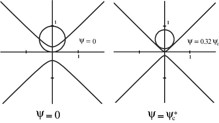
Figure 13: For generally anisotropic Dirac quasiparticles, the construction used in Fig.12 is modified to contain a hyperbola and circle. When these no longer intersect, the excitation spectrum becomes gapped. Illustrated is the construction for scattering parameter values $\{V_{1},R_{2},R_{3}\}=\{110,0.9,0.8\}$, impurity fraction $z=0.01$, and with $v_{f}=4v_{\Delta}$. For these parameters it was determined that the value of $\psi$ at which the spectrum becomes gapped is given by $\psi_{c}^{*}=0.32\psi_{c}$.

The value of $\psi$ at which these equations no longer have a solution is $\psi_{c}^{*}$. The computed values for $\psi_{c}^{*}$ are included for comparison in the plots of thermal conductivity in Fig. 14 and Fig. 15.

V.3 Effect of Self-Consistent Disorder

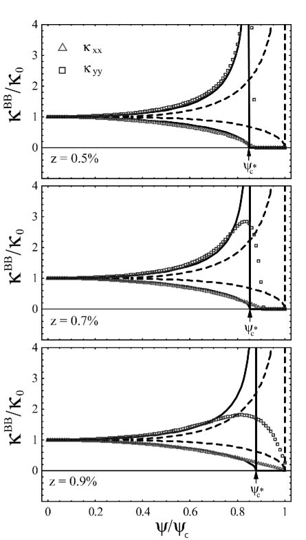
Figure 14: Effects of disorder on the charge-order-dependence of the bare-bubble thermal conductivity, isotropic case ($v_{f}=v_{\Delta}$). Note how an increase in the impurity fraction, $z$, broadens out the peak in the conductivity. As the disorder becomes sufficiently small, the computed conductivity (triangles and squares) attains a limiting value that closely agrees with the closed-form clean-limit results of Eq. (V.2.1) (shown with solid lines). The thermal conductivity obtained by simply letting $\widetilde{\Sigma}\rightarrow$-i$\Gamma_{0}$ (as in Ref. dur02, ) is shown with dashed lines. The effect of the self-consistent disorder is to renormalize the effective $\psi$ at which the thermal conductivity vanishes (from $\psi_{c}$ to $\psi_{c}^{*}$). Here, we have considered short-ranged scatterers $\{V_{1},R_{2},R_{3}\}=\{110,0.9,0.8\}$.

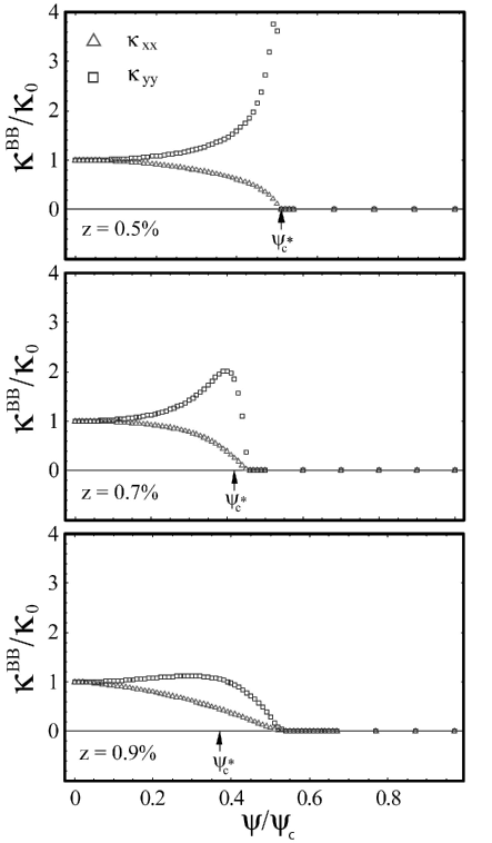
Figure 15: Effects of disorder on the charge-order-dependence of the bare-bubble thermal conductivity, anisotropic case ($v_{f}=16v_{\Delta}$). The effect of disorder is the same as in the isotropic case, which is to mix gapped and gapless states, smearing the peak in $\kappa_{yy}$ across the renormalized nodal transition point, $\psi_{c}^{*}$. It is interesting to note that for this anisotropic case, $\psi_{c}^{*}$ is significantly smaller than $\psi_{c}$. Again, we have considered short-ranged scatterers $\{V_{1},R_{2},R_{3}\}=\{110,0.9,0.8\}$.

Satisfied that vertex corrections are of little importance, we set about analyzing the form of the thermal conductivity by studying the bare-bubble results. Thermal conductivity $\kappa$ was computed for $\beta\equiv\sqrt{v_{f}/v_{\Delta}}$ values of $1,2,3$ and $4$ (that is, for $v_{f}/v_{\Delta}$=$1,4,9$ and $16$). In Fig. 14 is presented a representative plot of $\kappa$ for $v_{f}=v_{\Delta}$. The clean limit prediction for $\kappa$ (Eq. (V.2.1)) is computed by fitting $b_{1}$ and $b_{3}$ from the self-energy calculations. These clean limit predictions are then plotted on the same graph with the numerical results of the thermal conductivity for the same parameters. In addition, the clean limit results of the simpler disorder model of Ref. dur02, are also shown for the $v_{f}=v_{\Delta}$ case. Increasing disorder broadens the peak in $\kappa^{yy}$ near $\psi_{c}^{*}$. For $z=0.005$, the numerical computation is already almost exactly given by the clean limit results, while for $z=0.009$, the features of the conductivity are nearly totally smeared out, as seen in Fig. 14. In this figure, the value of $\psi_{c}^{*}$ given by Eq. (59) is indicated with an arrow.

For $v_{f}>v_{\Delta}$, the thermal conductivity has the same characteristics as for $v_{f}=v_{\Delta}$, except that $\psi_{c}^{*}$ is generally smaller for larger $\beta$. The numerically computed thermal conductivities for the case of $\beta=4$ are shown in Fig. 15. In this figure, the value of $\psi_{c}^{*}$ is computed by determining the largest value of $\psi$ for which Eqs. (V.2.2) have a solution, and is indicated with an arrow. It is clear from these graphs that the self-consistent disorder renormalizes the amplitude of charge density wave at which the thermal conductivity vanishes, and that the amount of renormalization is heavily dependent on the velocity anisotropy ratio, and varies only slightly with changing impurity fraction.

VI Conclusions

The work described in this paper investigates the low temperature thermal conductivity of a $d$-wave superconductor with coexisting charge order in the presence of impurity scattering. We improve upon the model studied in Ref. dur02, by incorporating the effect of vertex corrections, and by including disorder in a self-consistent manner. Inclusion of vertex corrections does not significantly modify the bare-bubble results for short range scattering potentials. The role vertex corrections play increases somewhat for longer range scattering potentials, in particular as the amplitude of charge ordering increases. Nonetheless, for reasonable parameter values, the inclusion of vertex corrections is not found to significantly modify the bare-bubble results. This opens up the possibility of doing bare-bubble calculations for models with different types of ordering.

Our analysis determined that for self-consistency, it is necessary to include off-diagonal (in extended-Nambu space) terms in the self-energy. As the charge ordering increases, the off-diagonal components become more important, and are found to dominate the self-energy in the clean limit. We also find that the zero-temperature thermal conductivity is no longer universal, as it depends on both disorder and charge order, rather than being solely determined by the anisotropy of the nodal energy spectrum.

In addition, inclusion of disorder within the self-consistent Born approximation renormalizes, generally to smaller values, the critical value of charge ordering strength $\psi$ at which the system becomes becomes effectively gapped. This renormalization is seen in the calculated thermal conductivity curves, and depends primarily on the impurity fraction $z$ and velocity anisotropy $v_{f}/v_{\Delta}$. For larger $v_{f}/v_{\Delta}$, the renormalization can be significant, which may indicate that the calculated effects could be seen in low-temperature thermal transport even in systems with relatively weak charge order.

Appendix A Self-consistent Green’s functions

Here are the Green’s functions that fulfill the self-consistent Born approximation. The superscript ⁽³⁾ refers to the fact that 3 successive applications of our self-energy scheme were necessary for self-consistency, as is explained in Section III.

$$G_{\mathrm{den}}^{(3)}(\omega)=\left(-f_{1}^{2}+f_{2}^{2}+f_{3}^{2}+(\psi_{c}+\beta p_{1})^{2}+(\frac{1}{\beta}p_{2})^{2}\right)\left(-f_{1}^{2}+f_{2}^{2}+f_{3}^{2}+(\psi_{c}+\beta p_{2})^{2}+(\frac{1}{\beta}p_{1})^{2}\right)$$

$$+4\left(f_{2}^{2}((\psi_{c}+\beta p_{1})(\psi_{c}+\beta p_{2})-\frac{1}{\beta^{2}}p_{1}p_{2}))-f_{3}\frac{1}{\beta}((\psi_{c}+\beta p_{1})p_{1}+(\psi_{c}+\beta p_{2})p_{2})\right)$$

$$-(f_{2}^{2}+f_{3}^{2})\Big{(}(2\psi_{c}+\beta(p_{1}+p_{2}))^{2}+\frac{1}{\beta^{2}}(p_{2}-p_{1})^{2}\Big{)}$$

$$\mathcal{G}_{A0}^{(3)}(\omega;p_{1},p_{2}) = -f_{1}\left(-f_{1}^{2}+(\psi_{c}+\beta p_{2})^{2}+\frac{1}{\beta^{2}}p_{1}^{2}+f_{2}^{2}+f_{3}^{2}\right)$$

$$\mathcal{G}_{A1}^{(3)}(\omega;p_{1},p_{2}) =- \frac{1}{\beta}p_{2}\left(-f_{1}^{2}+(\psi_{c}+\beta p_{2})^{2}+(\frac{1}{\beta}p_{1})^{2}\right)-\frac{1}{\beta}p_{1}(f_{3}^{2}-f_{2}^{2})+2(\psi_{c}+\beta p_{2})f_{2}f_{3}$$

$$\mathcal{G}_{A3}^{(3)}(\omega;p_{1},p_{2}) = -(\psi_{c}+\beta p_{1})\left(-f_{1}^{2}+(\psi_{c}+\beta p_{2})^{2}+(\frac{1}{\beta}p_{1})^{2}\right)+(\psi_{c}+\beta p_{2})(f_{3}^{2}-f_{2}^{2})+\frac{2}{\beta}p_{1}f_{2}f_{3}$$

$$\mathcal{G}_{B0}^{(3)}(\omega;p_{1},p_{2}) = f_{1}\left(f_{3}(2\psi_{c}+\beta(p_{1}+p_{2}))+f_{2}\frac{1}{\beta}(p_{1}+p_{2})\right)$$

$$\mathcal{G}_{B1}^{(3)}(\omega;p_{1},p_{2}) = f_{2}\left(f_{1}^{2}-(\psi_{c}+\beta p_{1})(\psi_{c}+\beta p_{2})+\frac{1}{\beta^{2}}p_{1}p_{2}-f_{2}^{2}-f_{3}^{2}\right)+f_{3}\Big{(}(\psi_{c}+\beta p_{1})p_{1}+(\psi_{c}+\beta p_{2})p_{2}\Big{)}$$

$$\mathcal{G}_{B2}^{(3)}(\omega;p_{1},p_{2}) = f_{1}\left(f_{3}(\frac{1}{\beta}p_{2}-\frac{1}{\beta}p_{1})+f_{2}\beta(p_{2}-p_{1})\right)$$

$$\mathcal{G}_{B3}^{(3)}(\omega;p_{1},p_{2}) = f_{3}\left(f_{1}^{2}-f_{2}^{2}-f_{3}^{2}+(\psi_{c}+\beta p_{1})(\psi_{c}+\beta p_{2})-\frac{1}{\beta^{2}}p_{1}p_{2}\right)+f_{2}\Big{(}(\psi_{c}+\beta p_{1})p_{1}+(\psi_{c}+\beta p_{2})p_{2})\Big{)}$$

$$\mathcal{G}_{C0}^{(3)}(\omega;p_{1},p_{2}) = \mathcal{G}_{B0}^{(3)}(\omega;p_{1},p_{2})$$

$$\mathcal{G}_{C1}^{(3)}(\omega;p_{1},p_{2}) = \mathcal{G}_{B1}^{(3)}(\omega;p_{1},p_{2})$$

$$\mathcal{G}_{C2}^{(3)}(\omega;p_{1},p_{2}) = -\mathcal{G}_{B2}^{(3)}(\omega;p_{1},p_{2})$$

$$\mathcal{G}_{C3}^{(3)}(\omega;p_{1},p_{2}) = \mathcal{G}_{B3}^{(3)}(\omega;p_{1},p_{2})$$

$$\mathcal{G}_{D0}^{(3)}(\omega;p_{1},p_{2}) = \mathcal{G}_{A0}^{(3)}(\omega;p_{2},p_{1})$$

$$\mathcal{G}_{D1}^{(3)}(\omega;p_{1},p_{2}) = \mathcal{G}_{C1}^{(3)}(\omega;p_{2},p_{1})$$

$$\mathcal{G}_{D3}^{(3)}(\omega;p_{1},p_{2}) = \mathcal{G}_{C3}^{(3)}(\omega;p_{2},p_{1})$$ (69)

To obtain the retarded Green’s function $G^{\mathrm{Ret}}(\omega)$ from the above we set

$$f_{1}=\omega-\Sigma_{A0}^{\mathrm{Ret}}(\omega)\hskip 10.0pt$$

$$f_{2}=\Sigma_{B1}^{\mathrm{Ret}}(\omega)\hskip 10.0pt$$

$$f_{3}=\psi+\Sigma_{B3}^{\mathrm{Ret}}(\omega).$$ (70)

For the retarded Green’s function $G^{\mathrm{Ret}}(\omega+\Omega)$, we set $\omega\rightarrow\omega+\Omega$, and for the advanced Green’s function $G^{\mathrm{Adv}}(\omega)$ we set $\Sigma^{\mathrm{Ret}}\rightarrow\Sigma^{\mathrm{Adv}}$ by taking the complex conjugate.

Appendix B Cutoff-Dependence of Self-Energy

Here we note that the self-consistent Born approximation, when applied to the nodal Green’s functions used in this paper, produces a self-energy that contains a logarithmic divergence, and therefore has a prefactor that is proportional to the momentum cutoff, set by the size of the Brillouin zone. By contrast, the thermal conductivity has no such dependence, and is therefore a truly nodal property. One difficulty this introduces is that the prefactor of the self-energy is sensitive to our choice of coordinates. As the location of the nodes evolves with charge density wave order parameter $\psi$, computations are necessarily performed in a different local coordinate system (than one centered about a node itself). This coordinate shift in the $p_{1}$ direction introduces a constant $\widetilde{\Sigma}_{A3}$ term, even in the $\psi=0$ instance (whereas using node-centered coordinates, the anti-symmetric integral is found to vanish). In the $\psi=0$ case, a shift of $\epsilon$ corresponds to the integral

$$I=\int_{-p_{0}+\epsilon}^{p_{0}+\epsilon}\mathrm{d}p_{1}\int_{-p_{0}}^{p_{0}}\mathrm{d}p_{2}\frac{p_{1}}{p_{1}^{2}+p_{2}^{2}+\Gamma_{0}^{2}}.$$ (71)

The result is $\pi\epsilon$, which matches the discrepancy. We therefore subtract off the $\psi=0$ value of $\widetilde{\Sigma}_{A3}$; the results shown in Fig. 3 reflect this recalibration, as do the subsequent iterations of the self-energy calculation.

Appendix C Calculation of Clean Limit Integral

For the clean limit of the thermal conductivity we need the integral

$$I=\int\frac{\mathrm{d}^{2}q}{4\pi}\frac{A}{\Big{(}k_{1}A+(q_{2}-k_{2})^{2}+\frac{1}{4}(q^{2}-k_{3})^{2}\Big{)}^{2}},$$ (72)

in the limit $A\rightarrow 0$. With the substitution

$$x_{1}\equiv x\cos\theta=q_{1}-1\hskip 30.0ptx_{2}\equiv x\sin\theta=q_{2}$$ (73)

the quantity $Y_{1}\equiv(q_{2}-k_{2})^{2}+\frac{1}{4}(q^{2}-k_{3}^{2})^{2}$ becomes

$$Y_{1} = \frac{x^{4}}{4}+k_{2}^{2}+\Big{(}\frac{1-k_{3}}{2}\Big{)}^{2}+\frac{1-k_{3}}{2}x^{2}+x^{2}$$ (74)

$$+(x^{2}+1-k_{3})x\cos\theta-2xk_{2}\sin\theta.$$

To simplify the angular integrand, we get rid of the $\sin\theta$ term by shifting $\theta\rightarrow\theta+\alpha$. Then, the last two terms of Eq. 74 become

$$\frac{x^{2}+1-k_{3}}{2}\cos(\theta+\alpha)-k_{2}\sin(\theta+\alpha)=(\frac{x^{2}+1-k_{3}}{2}\cos\alpha - k_{2}\sin\alpha)\cos\theta$$

$$-(\frac{x^{2}+1-k_{3}}{2}\sin\alpha+k_{2}\cos\alpha)\sin\theta.$$ (75)

We set the coefficient of the second term on the RHS of Eq. (75) to $0$, so that the first term becomes

$$-\frac{1}{k_{2}}\Big{(}(\frac{x^{2}+1-k_{3}}{2})^{2}+k_{2}^{2}\Big{)}\sin\alpha\cos\theta=\frac{-1}{r}\Big{(}\frac{x^{4}}{4}+\frac{1-k_{3}}{2}x^{2}+(\frac{1-k_{3}}{2})^{2}+k_{2}^{2}\Big{)}\cos\theta,$$ (76)

where the RHS of Eq. (76) is obtained by setting $\sin\alpha\equiv k_{2}/r$, where $r=r(x)$ is an undetermined function of $x$. With this substitution, Eq. (74) becomes

$$\frac{x^{4}}{4}+\frac{1-k_{3}}{2}x^{2}+(\frac{1-k_{3}}{2})^{2}+k_{2}^{2}+x^{2}-\frac{2x}{r}\Big{(}\frac{x^{4}}{4} + \frac{1-k_{3}}{2}x^{2}+(\frac{1-k_{3}}{2})^{2}+k_{2}^{2}\Big{)}\cos(\theta+\alpha)$$ (77)

$$= \Big{(}(\frac{x^{2}+1-k_{3}}{2})^{2}+k_{2}^{2}\Big{)}\Big{(}1+\frac{x^{2}}{(\frac{x^{2}+1-k_{3}}{2})^{2}+k_{2}^{2}}-\frac{2x}{r}\cos(\theta+\alpha)\Big{)}$$

$$= \frac{x^{2}}{a^{2}}\Big{(}1+a^{2}-2a\cos(\theta+\alpha)\Big{)},$$

where

$$r=\sqrt{\Big{(}\frac{x^{2}+1-k_{3}}{2}\Big{)}^{2}+k_{2}^{2}}\hskip 20.0pt\mathrm{and}\hskip 20.0pta=\frac{x}{r}.$$ (78)

Then, defining $\gamma=k_{1}a^{2}/x^{2}$, the integral of Eq. (72) becomes

$$I =\int\frac{\mathrm{d}^{2}x}{4\pi}\frac{A}{\Big{(}k_{1}A+\frac{x^{2}}{a^{2}}(1+a^{2}-2a\cos(\theta+\alpha))\Big{)}^{2}}$$ (79)

$$= \int_{0}^{\infty}\frac{x\mathrm{d}x}{2\pi}\frac{a^{4}}{x^{4}}\int_{0}^{\pi}\frac{A\,\,\mathrm{d}\theta}{\Big{(}A\gamma+1+a^{2}-2a\cos(\theta+\alpha)\Big{)}^{2}}$$

after shifting $\theta\rightarrow\theta-\alpha$, and noting the evenness of the $\theta$ integral. The integral is found in standard integration tablesGradshteyn , and noting that $(1\pm a)^{2}+A\gamma\geq 0$, we obtain

$$I=\int_{0}^{\infty}\frac{\mathrm{d}x}{2\pi}\frac{a^{4}}{x^{3}}\frac{A\pi(1+a^{2})}{(1+a)^{3}}\Big{(}(1-a)^{2}+A\gamma\Big{)}^{-3/2}.$$ (80)

Since in the limit that $A\rightarrow 0$,

$$\frac{A}{\Big{(}(1+a)^{2}+A\gamma\Big{)}^{3/2}}\rightarrow\frac{2}{\gamma}\delta(1-a),$$ (81)

we find that

$$I=\int_{0}^{\infty}\frac{\mathrm{d}x}{4k_{1}}\frac{x}{\Big{(}\frac{x^{2}+1-k_{3}}{2}\Big{)}^{2}+k_{2}^{2}}\,\,\delta(a-1).$$ (82)

Making the further substitution $y=(x^{2}+1-k_{3})/2$,

$$I = \int_{\stackrel{{\scriptstyle\underline{1-k_{3}}}}{{2}}}^{\infty}\,\,\frac{\mathrm{d}y}{2k_{1}}\frac{1}{y^{2}+k_{2}^{2}}\,\,\delta\,\Big{(}\frac{2y-(1-k_{3})}{(y^{2}+k_{2}^{2})^{2}}-1\Big{)}$$ (83)

$$= \int_{\stackrel{{\scriptstyle\underline{1-k_{3}}}}{{2}}}^{\infty}\,\,\frac{\mathrm{d}y}{4k_{1}}\frac{y^{2}+k_{2}^{2}}{\Big{|}k_{2}^{2}-y^{2}+y(1-k_{3})\Big{|}}$$

$$\times\Big{(}\delta(y-y_{+})+\delta(y-y_{-})\Big{)},$$

where

$$y_{\pm}=1\pm\sqrt{k_{3}-k_{2}^{2}}$$ (84)

are the intersections of the curves $y^{2}+k_{2}^{2}$ and $2y-(1-k_{3})$. It is easily verified that both $y_{+}$ and $y_{-}$ are in the range of integration $\bf{[}\frac{1-k_{3}}{2},\infty\bf{)}$ ($y_{-}$ just catching the lower bound when $\psi=0$). Then expanding the denominator of Eq. (83) using Eq. (84), we find

$$\Big{|}k_{2}^{2}-y_{\pm}^{2}+y_{\pm}(1-k_{3})\Big{|}=2\sqrt{k_{3}-k_{2}^{2}}\,\,\Big{|}\sqrt{k_{3}-k_{2}^{2}}\pm\frac{1+k_{3}}{2}\Big{|}$$ (85)

so that

$$I = \frac{1}{2k_{1}}\frac{1}{2\sqrt{k_{3}-k_{2}^{2}}}\Big{(}\frac{1+k_{3}+2\sqrt{k_{3}-k_{2}^{2}}}{1+k_{3}+2\sqrt{k_{3}-k_{2}^{2}}}+\frac{1+k_{3}-2\sqrt{k_{3}-k_{2}^{2}}}{1+k_{3}-2\sqrt{k_{3}-k_{2}^{2}}}\Big{)}$$ (86)

$$= \frac{1}{2k_{1}\sqrt{k_{3}-k_{2}^{2}}}$$

References

- (1) D.J. Van Harlingen, Rev. Mod. Phys. 67 515 (1995).
- (2) P.A. Lee, Science 277, 50 (1997).
- (3) A. Altland, B.D. Simons and M.R. Zirnbauer, Phys. Reports 359 283 (2002)
- (4) J. Orenstein and A.J. Millis, Science 288, 468 (2000).
- (5) L.P. Gor’kov and P.A. Kalugin, Pis’ma Zh. ksp. Teor. Fiz. 41, 208 (1985) [JETP Lett. 41, 253 (1985)]
- (6) P.A. Lee, Phys. Rev. Lett. 71, 1887 (1993).
- (7) P.J. Hirschfeld, W.O. Putikka and D.J. Scalapino, Phys. Rev. Lett. 71, 3705 (1993).
- (8) P.J. Hirschfeld, W.O. Putikka and D.J. Scalapino, Phys. Rev. B 50, 10250 (1994).
- (9) P.J. Hirschfeld and W.O. Putikka, Phys. Rev. Lett. 77, 3909 (1996).
- (10) M.J. Graf, S-K. Yip., J.A. Sauls and D. Rainier, Phys. Rev. B 53 15147 (1996).
- (11) T. Senthil, M.P.A. Fisher, L. Balents and C. Nayak, Phys. Rev. Lett. 81, 4704 (1998).
- (12) A.C. Durst and P.A. Lee, Phys. Rev. B 62 1270 (2000).
- (13) L. Taillefer, B. Lussier, R. Gagnon, K. Behnia and H. Aubin, Phys. Rev. Lett. 79, 483 (1997).
- (14) M. Chiao, R.W. Hill, C. Lupien, B. Popi, R. Gagnon and L. Taillefer, Phys. Rev. Lett. 82 2943 (1999)
- (15) M. Chiao, R.W. Hill, C. Lupien, L. Taillefer, P. Lambert, R. Gagnon and P. Fournier, Phys. Rev. B 62 3554 (2000)
- (16) S. Nakamae, K. Behnia, L. Balicas, F. Rullier-Albenque, H. Berger and T. Tamegai, Phys. Rev. B 63 184509 (2001)
- (17) C. Proust, E. Boaknin, R.W. Hill, L. Taillefer and A.P. Mackenzie, Phys. Rev. Lett. 89, 147003 (2002).
- (18) M. Sutherland, D.G. Hawthorn, R.W. Hill, F. Ronning, S. Wakimoto, H. Zhang, C. Proust, E. Boaknin, C. Lupien, L. Taillefer, R.X. Liang, D.A. Bonn, W.N. Hardy, R. Gagnon, N.E. Hussey, T. Kimura, M. Nohara and H. Tagaki, Phys. Rev. B 67 174520 (2003)
- (19) R.W. Hill, C. Lupien, M. Sutherland, E. Boaknin, D.G. Hawthorn, C. Proust, F. Ronning, L. Taillefer, R. Liang, D.A. Bonn and W.N. Hardy, Phys. Rev. Lett. 92, 027001 (2004).
- (20) X.F. Sun, K. Segawa and Y. Ando, Phys. Rev. Lett. 93, 107001 (2004).
- (21) M. Sutherland, S.Y. Li, D.G. Hawthorn, R.W. Hill, F. Ronning, M.A. Tanatar, J. Paglione, H. Zhang, L. Taillefer, J. DeBenedictis, R. Liang, D.A. Bonn and W.N. Hardy, Phys. Rev. Lett. 94, 147004 (2005).
- (22) D.G. Hawthorn, S.Y. Li, M. Sutherland, E. Boaknin, R.W. Hill, C. Proust, F. Ronning, M.A. Tanatar, J.P. Paglione, L. Taillefer, D. Peets, R.X. Liang, D.A. Bonn, W.N. Hardy and N.N. Kolesnikov, Phys. Rev. B 75 104518 (2007)
- (23) X.F. Sun, S. Ono, X. Zhao, Z.Q. Pang, Y. Abe and Y. Ando, Phys. Rev. B 77 094515 (2008).
- (24) S.A. Kivelson, I.P. Bindloss, E. Fradkin, V. Oganesyan, J.M. Tranquada, A. Kapitulnik and C. Howald, Rev. Mod. Phys. 75, 1201 (2003) (and references within)
- (25) D. Podolsky, E. Demler, K. Damle and B.I. Halperin, Phys. Rev. B 67 094514 (2003)
- (26) J.X. Li, C.Q. Wu and D.H. Lee, Phys. Rev. B 74 184515 (2006)
- (27) C.T. Chen, A.D. Beyer and N.C. Yeh, Solid State Communications 143 447 (2007)
- (28) K.J. Seo, H.D. Chen, and J.P. Hu, Phys. Rev. B 76 020511 (R) (2007)
- (29) J.E. Hoffmann, E.W. Hudson, K.M. Lang, V. Madhavan, H. Eisaki, S. Uchida, and J.C. Davis, Science 295 466 (2002).
- (30) J.E. Hoffmann, K. McElroy, D.H. Lee, K.M. Lang, H. Eisaki, S. Uchida and J.C. Davis, Science 297, 1148 (2002).
- (31) C. Howald, H. Eisaki, N. Kaneko, M. Greven and A. Kapitulnik, Phys. Rev. B 67 014533 (2003).
- (32) M. Vershinin, S. Misra, S. Ono, Y. Abe, Y. Ando and A. Yazdani, Science 303, 1995 (2004).
- (33) K. McElroy, D.H. Lee, J.E. Hoffman, K.M. Lang, J. Lee, E.W. Hudson, H. Eisaki, S. Uchida, and J.C. Davis, Phys. Rev. Lett. 94, 197005 (2005).
- (34) T. Hanaguri, C. Lupien, Y. Kohsaka, D.H. Lee, M. Azuma, M. Takano, H. Takagi and J.C. Davis, Nature 430 1001 (2004).
- (35) S. Misra, M. Vershenin, P. Phillips and A. Yazdani, Phys. Rev. B 70 220503(R) (2004).
- (36) K. McElroy, D.H. Lee, J.E. Hoffman, K.M. Lang, J. Lee, E.W. Hudson, H. Eisaki, S. Uchida and J.C. Davis, Phys. Rev. Lett. 94, 197005 (2005).
- (37) Y. Kohsaka, C. Taylor, K. Fujita, A. Schmidt, C. Lupien, T. Hanaguri, M. Azuma, M. Takano, H. Eisaki, H. Takagi, S. Uchida and J.C. Davis, Science 315, 1380 (2007).
- (38) M.C. Boyer, W.D. Wise, K. Chatterjee, M. Yi, T. Kondo, T. Takeuchi, H. Ikuta and E.W. Hudson, Nature Physics 3, 802 (2007).
- (39) T. Hanguri, Y. Kohsaka, J.C. Davis, C. Lupien, I. Yamada, M. Azuma, M. Takano, K. Ohishi, M. Ono and H. Takagi, Nature Physics 3, 865 (2007).
- (40) A.N. Pasupathy, A. Pushp, K.K. Gomes, C.V. Parker, J. Wen, Z. Xu, G. Gu, S. Ono, Y. Ando and A. Yazdani, Science 320, 196 (2008).
- (41) W.D. Wise, M.C. Boyer, K. Chatterjee, T. Kondo, T. Takeuchi, H. Ikuta, Y. Wang and E.W. Hudson, Nature Physics 4, 696 (2008).
- (42) Y. Kohsaka, C. Taylor, P. Wahi, A. Schmidt, J. Lee, K. Fujita, J.W. Allredge, K. McElroy, J. Lee, H. Eisaki, S. Uchida, D.H. Lee and J.C. Davis, Nature 454, 1072 (2008).
- (43) E. Berg, C.C. Chen and S.A. Kivelson, Phys. Rev. Lett. 100 027003 (2008)
- (44) K. Park and S. Sachdev, Phys. Rev. B 64 184510 (2001)
- (45) M. Granath, V. Oganesyan, S. A. Kivelson, E. Fradkin, and V. J. Emery, Phys. Rev. Lett. 86, 167011 (2001)
- (46) M. Vojta, Y. Zhang and S. Sachdev, PhysṘev. B 62 6721 (2000)
- (47) A. C. Durst and S. Sachdev, arXiv:0810.3914 (2008)
- (48) N.E. Hussey, Advances in Physics 51, 1685 (2002).
- (49) J. Takeya, Y. Ando, S. Komiya, an X. F. Sun, Phys. Rev. Lett. 88, 077001 (2002).
- (50) X. F. Sun, S. Komiya, J. Takeya, and Y. Ando, Phys. Rev. Lett. 90, 117004 (2003).
- (51) Y. Ando, S. Ono, X.F. Sun, J. Takeya, F.F. Balakirev, J.B. Betts and G.S. Boebinger, Phys. Rev. Lett. 92, 247004 (2004).
- (52) X.F. Sun, K. Segawa and Y. Ando, Phys. Rev. B 72, 100502 (2005).
- (53) X.F. Sun, S. Ono, Y. Abe, S. Komiya, K. Segawa and Y. Ando, Phys. Rev. Lett. 96, 017008 (2006).
- (54) D.G. Hawthorn, R.W. Hill, C. Proust, F. Ronning, M. Sutherland, E. Boaknin, C. Lupien, M.A. Tanatar, J. Paglione, S. Wakimoto, H. Zhang, L. Taillefer, T. Kimura, M. Nohara and N.E. Hussey, Phys. Rev. Lett. 90, 197004 (2003).
- (55) V. P. Gusynin and V. A. Miransky, Eur. Phys. J. B 37, 363 (2004).
- (56) B. M. Andersen and P. J. Hirschfeld, Phys. Rev. Lett. 100, 257003 (2008).
- (57) G. D. Mahan, Many-Particle Physics (Plenum Press, New York, 1981).
- (58) A. L. Fetter and J. D. Walecka, Quantum Theory of Many-Particle Systems (McGraw Hill, Boston, 1971).
- (59) I. S. Gradshteyn and I. M. Ryzhik, Table of Integrals, Series and Products (Academic Press, San Diego, 1994).