Computing the Newton Polygon
of the Implicit Equation

Abstract

We consider polynomially and rationally parameterized curves, where the polynomials in the parameterization have fixed supports and generic coefficients. We apply sparse (or toric) elimination theory in order to determine the vertex representation of its implicit polygon, i.e. of the implicit equation’s Newton polygon. In particular, we consider mixed subdivisions of the input Newton polygons and regular triangulations of point sets defined by Cayley’s trick. We distinguish polynomial and rational parameterizations, where the latter may have the same or different denominators; the implicit polygon is shown to have, respectively, up to 4, 5, or 6 vertices. In certain cases, we also determine some of the coefficients in the implicit equation.

Keywords: Sparse (toric) resultant, implicitization, Newton polygon, Cayley trick, mixed subdivision.

1 Introduction

Implicitization is the problem of switching from a parametric representation of a hypersurface to an algebraic one. It is a fundamental question with several applications, e.g. [Hof89, HSW97]. Here we consider the implicitization problem for a planar curve, where the polynomials in its parameterization have fixed Newton polytopes. We determine the vertices of the Newton polygon of the implicit equation, or implicit polygon, without computing the equation, under the assumption of generic coefficients relative to the given supports, i.e. our results hold for all coefficient vectors in some open dense subset of the coefficient space.

This problem was posed in [SY94]. It appeared in [EK03, EK05], then in [STY07, SY07], and more recently in [EK07] and [DS07]. The motivation is that “apriori knowledge of the Newton polytope would greatly facilitate the subsequent computation of recovering the coefficients of the implicit equation […] This is a problem of numerical linear algebra …”[[STY07]]. Reducing implicitization to linear algebra is also the premise of [CGKW01, EK03]. Yet, this can be nontrivial if coefficients are not generic.Another potential application of knowing the implicit polygon is to approximate implicitization, see [Dok01].

Previous work includes [EK03, EK05], where an algorithm constructs the Newton polytope of any implicit equation. That method had to compute all mixed subdivisions, then applies cor. 3. In [GKZ94, chapter 12], the authors study the resultant of two univariate polynomials and describe the facets of its Newton polytope. In [GKZ90], the extreme monomials of the Sylvester resultant are described. The approaches in [EK03, GKZ94], cannot exploit the fact that the denominators in a rational parameterization may be identical.

[STY07] offered algorithms to compute the Newton polytope of the implicit equation of any hypersurface parameterized by Laurent polynomials. Their approach is based on tropical geometry. It extends to arbitrary implicit ideals. They give a generically optimal implicit support; for curves, the support is described in [STY07, example 1.1]. Their approach also handles rational parameterizations with the same denominator by homogenizing the parameter as well as the implicit space. The implicit equation is homogeneous, hence its Newton polytope lies in a hyperplane, which may cause numerical instability in the computation.

In [EK07] the problem is solved in an abstract way by means of composite bodies and mixed fiber polytopes. In [DS07] the normal fan of the implicit polygon is determined, with no genericity assumption on the coefficients. This is computed by the multiplicities of any parameterization of the rational plane curve. The authors are based on a refinement of the famous Kushnirenko-Bernstein formula for the computation of the isolated roots of a polynomial system in the torus, given in [PS07]. As a corollary, they obtain the optimal implicit polygon in case of generic coefficients. They also address the inverse question, namely when can a given polygon be the Newton polygon of an implicit curve.

In many applications, such as computing the $u$-resultant or in implicitization, the resultant coefficients are themselves polynomials in a few parameters, and we wish to study the resultant as a polynomial in these parameters. In [EKP07], we computed the Newton polytope of specialized resultants while avoiding to compute the entire secondary polytope; our approach was to examine the silhouette of the latter with respect to an orthogonal projection. We presented a method to compute the vertices of the implicit polygon of polynomial or rational parametric curves, when denominators differ. We also introduced a method and gave partial results for the case when denominators are equal; the latter method is fully developed in the present article.

Our main contribution is to determine the vertex structure of the implicit polygon. This polygon is optimal if the coefficients of the parametric polynomials are sufficiently generic with respect to the given supports, otherwise it contains the true polygon. Our presentation is self-contained. In the case of polynomially parameterized curves and rationally parameterized curves with different denominators (which includes the case of Laurent polynomial parameterizations), the Cayley trick reduces the problem to computing regular triangulations of point sets in the plane. In retrospect, our methods are similar to those employed in [GKZ90]. We also determine certain coefficients in the implicit equation. If the denominators are identical, two-dimensional mixed subdivisions are examined; we show that only subdivisions obtained by linear liftings are relevant.

The following proposition collects our main corollaries regarding the shape of the implicit polygon in terms of corner cuts on an initial polygon: $\phi$ is the implicit equation and $N(\phi)$ is the implicit polytope.

Proposition 1.

$N(\phi)$ is defined by a polygon with one vertex at the origin and two edges lying on the axes. In particular,
Polynomial parameterizations: $N(\phi)$ is defined by a right triangle with at most one corner cut, which excludes the origin.
Rational parameterizations with equal denominators: $N(\phi)$ is defined by a right triangle with at most two cuts, on the same or different corners.
Rational parameterizations with different denominators: $N(\phi)$ is defined by a quadrilateral with at most two cuts, on the same or different corners.

Example 1.

Consider:

$$x=\frac{t^{6}+2t^{2}}{t^{7}+1},y=\frac{t^{4}-t^{3}}{t^{7}+1},$$

Theorem 16 yields vertices $(7,0),(0,7),(0,3),(3,1),(6,0)$, which define the actual implicit polygon because the implicit equation is

$\phi=-32y^{4}-30x^{3}y^{2}-x^{4}y-12x^{2}y^{2}-3x^{3}y-7x^{6}y-2x^{7}+20xy^{3}+280x^{2}y^{5}-7^{3}y^{4}x-70x^{4}y^{3}-\\ 22x^{3}y^{3}-49x^{5}y^{2}-21x^{4}y^{2}+11x^{5}y+216y^{5}+129y^{7}-248y^{6}+70xy^{6}+185xy^{5}+24y^{3}+100xy^{4}+\\ 43x^{2}y^{3}+72x^{2}y^{4}+3x^{6}.\\$

Changing the coefficient of $t^{2}$ to -1, leads to an implicit polygon with 4 cuts which is contained in the polygon predicted by theorem 16. This shows the importance of the genericity condition on the coefficients of the parametric polynomials. See example 6 for details.

An instance where the implicit polygon has 6 vertices is:

$$x=\frac{t^{3}+2t^{2}+t}{t^{2}+3t-2},~{}y=\frac{t^{3}-t^{2}}{t-2}.$$

Our results in section 5 yield implicit vertices $\{(0,1),(0,3),(3,0),(1,3),(2,0),(3,2)\}$ which define the actual implicit polygon. See example 14 for details.

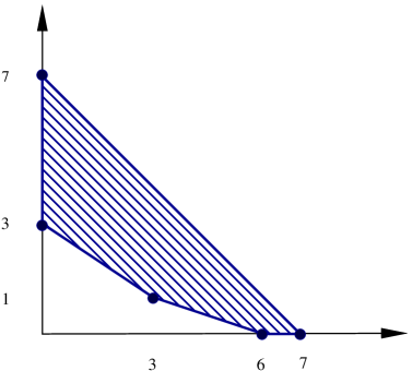
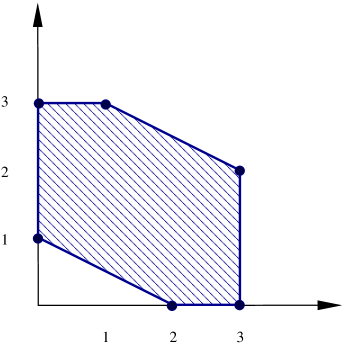
Figure 1: The implicit polygons of the curves of example 1.

The paper is organized as follows. The next section recalls concepts from sparse elimination and focuses on the Newton polytope of the sparse resultant. It also defines the problem of computing the implicit polytope. Section 3 solves the problem for rational parameterizations with identical denominators, by studying relevant mixed subdivisions. Section 4 determines the implicit polygon for polynomially parameterized curves. Section 5 refers to rational parametric curves, where denominators are different. We conclude with further work in section 6.

2 Sparse elimination and Implicitization

We first recall some notions of sparse elimination theory; see [GKZ94] for more information. Then, we define the problem of implicitization.

Given a polynomial $f$, its support $A(f)$ is the set of the exponent vectors corresponding to monomials with nonzero coefficients. Its Newton polytope $N(f)$ is the convex hull of $A(f)$, denoted CH$(A(f))$. The Minkowski sum $A+B$ of (convex polytopes) $A,B\subset\mathbb{R}^{n}$ is the set $A+B=\{a+b~{}|~{}a\in A,b\in B\}\subset\mathbb{R}^{n}.$

Definition 1.

Consider Laurent polynomials $f_{i},~{}i=0,\dots,n$, in $n$ variables, with fixed supports. Let $\mathrm{c}=(c_{0,0},\ldots,c_{0,s_{0}},\ldots,c_{n,0},\ldots,c_{n,s_{n}})$ be the vector of all nonzero (symbolic) coefficients. The sparse (or toric) resultant $\mathcal{R}$ of the $f_{i}$ is the unique, up to sign, irreducible polynomial in $\mathbb{Z}[\mathrm{c}]$, which vanishes iff the $f_{i}$ have a common root in the toric variety corresponding to the supports of the $f_{i}$.

Let the system’s Newton polytopes be $P_{0},\ldots,P_{n}\subset\mathbb{R}^{n}$. Their mixed volume is the unique integer-valued function, which is symmetric, multilinear with respect to Minkowski addition, and satisfies MV$(Q,\dots,Q)=n!$ Vol$(Q)$, for any lattice polytope $Q\subset\mathbb{R}^{n}$, where Vol$(\cdot)$ indicates Euclidean volume. For the rest of the paper we assume that the Minkowski sum $P=P_{0}+\cdots+P_{n}\subset\mathbb{R}^{n}$ is $n$-dimensional. The family of supports $A_{0},\dots,A_{n}$ is essential according to the terminology of [Stu94, sec. 1]. This is equivalent to the existence of a non-zero partial mixed volume MV${}_{i}=$ MV$(A_{0},\ldots,A_{i-1},A_{i+1},\ldots,A_{n})$, for some $i\in\{0,\dots,n\}$

A Minkowski cell of $P$ is any full-dimensional convex polytope $B=\sum_{i=0}^{n}B_{i}$, where each $B_{i}$ is a convex polytope with vertices in $A_{i}$. We say that two Minkowski cells $B=\sum_{i=0}^{n}B_{i}$ and $B^{\prime}=\sum_{i=0}^{n}B_{i}^{\prime}$ intersect properly when the intersection of the polytopes $B_{i}$ and $B_{i}^{\prime}$ is a face of both and their Minkowski sum descriptions are compatible, cf. [San05].

Definition 2.

[San05, definition 1.1] A mixed subdivision of $P$ is any family $S$ of Minkowski cells which partition $P$ and intersect properly as Minkowski sums. Cell $R$ is mixed, in particular $i$-mixed or $v_{i}$-mixed, if it is the Minkowski sum of $n$ one-dimensional segments $E_{j}\subset P_{j}$, which are called edge summands, and one vertex $v_{i}\in P_{i}$.

Note that mixed subdivisions contain faces of all dimensions between 0 and $n$, the maximum dimension corresponding to cells. Every face of a mixed subdivision of $P$ has a unique description as Minkowski sum of subpolytopes of the $P_{i}$’s. A mixed subdivision is called regular if it is obtained as the projection of the lower hull of the Minkowski sum of lifted polytopes $\{(p_{i},\omega_{i}(p_{i}))~{}|~{}p_{i}\in P_{i}\}$. If the lifting function $\omega:=\{\omega_{i}\ldots,\omega_{n}\}$ is sufficiently generic, then the induced mixed subdivision is called tight.

A monomial of the sparse resultant is called extreme if its exponent vector corresponds to a vertex of the Newton polytope $N(\mathcal{R})$ of the resultant. Let $\omega$ be a sufficiently generic lifting function. The $\omega$-extreme monomial of $\mathcal{R}$ is the monomial with exponent vector that maximizes the inner product with $\omega$; it corresponds to a vertex of $N(\mathcal{R})$ with outer normal vector $\omega$.

Proposition 2.

[Stu94]. For every sufficiently generic lifting function $\omega$, we obtain the $\omega$-extreme monomial of $\mathcal{R}$, of the form

$$\pm\prod_{i=0}^{n}\prod_{R}c_{i,v_{i}}^{\mathrm{Vol}(R)},$$ (1)

where ${\rm Vol}(R)$ is the Euclidean volume of $R$, the second product is over all $v_{i}$-mixed cells $R$ of the regular tight mixed subdivision of $P$ induced by $\omega$, and $c_{i,v_{i}}$ is the coefficient of the monomial of $f_{i}$ corresponding to vertex $v_{i}$.

Corollary 3.

There exists a surjection from the mixed cell configurations onto the set of extreme monomials of the sparse resultant.

Given supports $A_{0},\ldots,A_{n}$, the Cayley embedding $\kappa$ introduces a new point set

$$C:=\kappa\left(A_{0},A_{1},\ldots,A_{n}\right)=\bigcup_{i=0}^{n}(A_{i}\times\{e_{i}\})\subset\mathbb{R}^{2n},$$

where $e_{i}$ are an affine basis of $\mathbb{R}^{n}$.

Proposition 4.

[The Cayley Trick] [MV99, San05]. There exists a bijection between the regular tight mixed subdivisions of the Minkowski sum $P$ and the regular triangulations of $C$.

We now consider the general problem of implicitization. Let $h_{0},\ldots,h_{n}\in\mathbb{C}[t_{1},\ldots,t_{r}]$ be polynomials in parameters $t_{i}$. The implicitization problem is to compute the prime ideal $I$ of all polynomials $\phi\in\mathbb{C}[x_{0},\ldots,x_{n}]$ which satisfy $\phi(h_{0},\ldots,h_{n})\equiv 0$ in $\mathbb{C}[t_{1},\ldots,t_{r}]$. We are interested in the case where $r=n$, and generalize $h_{i}$ to be rational expressions in $\mathbb{C}(t_{1},\ldots,t_{n})$. Then $I=\langle\phi\rangle$ is a principal ideal. Note that $\phi\in\mathbb{C}[x_{0},\dots,x_{n}]$ is uniquely defined up to sign. The $x_{i}$ are called implicit variables, $A(\phi)$ is the implicit support and $N(\phi)$ is the implicit polytope. Usually a rational parameterization may be defined by

$$x_{i}=\frac{P_{i}(\mathrm{t})}{Q(\mathrm{t})},~{}i=0,\ldots,n,~{}~{}\gcd(P_{0}(\mathrm{t}),\ldots,P_{n}(\mathrm{t}),Q(\mathrm{t}))=1,~{}\mathrm{t}=(t_{1},\ldots,t_{n}).$$ (2)

Alternatively, the input may be

$$x_{i}=\frac{P_{i}(\mathrm{t})}{Q_{i}(\mathrm{t})},~{}i=0,\ldots,n,~{}~{}\gcd(P_{i}(\mathrm{t}),Q_{i}(\mathrm{t}))=1,~{}\mathrm{t}=(t_{1},\ldots,t_{n}).$$ (3)

In both cases, all polynomial have fixed supports. We assume that the degree of the parameterization equals 1. This avoids, e.g., having all terms in $t^{a}$ for some $a>1$.

Proposition 5.

Consider system (2) and let $S\subset\mathbb{Z}^{n}$ be the union of the supports of polynomials $x_{i}Q-P_{i}$. Then, the total degree of the implicit equation $\phi$ is bounded by the volume of the convex hull CH$(S)$ multiplied by $n!$. The degree of $\phi$ in $x_{j}$ is bounded by the mixed volume of the $f_{i},~{}i\neq j$.

When the rational parameterization is given by equations (3), we have the following.

Corollary 6.

Let $S=(A(P_{i})+\sum_{j=0,j\neq i}^{n}A(Q_{j}))\cup(\sum_{i=0}^{n}A(Q_{i}))$. The total degree of the implicit equation $\phi$ is bounded by the volume of the convex hull CH$(S)$ multiplied by $n!$.

The implicit supports predicted solely by degree bounds are typically larger than optimal.

3 Rational parameterizations with equal denominators

We study rationally parameterized curves, when both denominators are the same.

$$x=\frac{P_{0}(t)}{Q(t)},~{}y=\frac{P_{1}(t)}{Q(t)},~{}~{}\gcd(P_{i}(t),Q(t))=1,\,P_{i},Q\in\mathbb{C}[t],\,i=0,1,$$ (4)

where the $P_{i},Q$ have fixed supports and generic coefficients. If some $P_{i}(t),Q(t)$ have a nontrivial GCD, then common terms are divided out and the problem reduces to the case of different denominators. In general, the $P_{i},Q$ are Laurent polynomials, but this case can be reduced to the case of polynomials by shifting the supports.

Applying the methods for the case of different denominators does not lead to optimal implicit support. The reason is that this does not exploit the fact that the coefficients of $Q(t)$ are the same in the polynomials $xQ-P_{0},yQ-P_{1}$. Therefore, we introduce a new variable $r$ and consider the following system

$$f_{0}=xr-P_{0}(t),\;f_{1}=yr-P_{1}(t),\;f_{2}=r-Q(t)\in\mathbb{C}[t,r].$$ (5)

By eliminating $t,r$ the resultant gives, for generic coefficients, the implicit equation in $x,y$. This is the de-homogenization of the resultant of $x_{0}-P_{0}^{h},x_{1}-P_{1}^{h},x_{2}-Q^{h}$, where $P_{0}^{h},P_{1}^{h},Q^{h}$ are the homogenizations of $P_{0},P_{1},Q$. This resultant is homogeneous in $x_{0},x_{1},x_{2}$ and generically equals the implicit equation $\Phi\in\mathbb{C}[x_{0},x_{1},x_{2}]$ of parameterization $\mathbb{P}\rightarrow\mathbb{P}^{2}:(t:t_{0})\mapsto(x_{0}:x_{1}:x_{2})=(P_{0}^{h}:P_{1}^{h}:Q^{h})$.

Let the input Newton segments be

$$B_{i}=N(P_{i}),i=0,1,\;B_{2}=N(Q),\mbox{ where }B_{i}=\{b_{iL},\dots,b_{iR}\},i=0,1,2,$$

where $b_{iL},~{}b_{iR}$ are the endpoints of segment $B_{i}$. The supports of the $f_{i}$ are

$$A_{0}=\{a_{00},a_{0L},\dots,a_{0R}\},A_{1}=\{a_{10},a_{1L},\dots,a_{1R}\},A_{2}=\{a_{20},a_{2L},\dots,a_{2R}\}\in\mathbb{N}^{2},$$

where

• each point $a_{i0}=(0,1)$, for $i=0,1,2$, corresponds to the unique term in $f_{i}$ which depends on $r$,

• each other point $a_{it}$, for $t\neq 0$, is of the form $(b_{it},0)$, for one $b_{it}\in B_{i}$.

One could think that index $L=1$ whereas each $R$ equals the cardinality of the respective $B_{i}$. By the above hypotheses either $A_{2}$ or both $A_{0},A_{1}$ contain $(0,0)$.

Lemma 7.

MV${}_{\mathbb{R}}(B_{i}\cup B_{j})=$ MV${}_{\mathbb{R}^{2}}(A_{i},A_{j}),~{}i,j\in\{0,1,2\}$, where MV${}_{\mathbb{R}^{d}}$ denotes mixed volume in $\mathbb{R}^{d}$.

Proof.

Let $B_{i}=[m_{i},l_{i}],~{}B_{j}=[m_{j},l_{j}]$ be intervals in $\mathbb{N}$. If $m_{i}\leq m_{j}$ and $l_{i}\leq l_{j}$, then MV${}_{\mathbb{R}}(B_{i}\cup B_{j})=l_{j}-m_{i}$. Consider a mixed subdivision of $A_{i}+A_{j}$, with unique mixed cell $((0,1),(m_{i},0))+((0,1),(l_{j},0))$, hence MV${}_{\mathbb{R}^{2}}(A_{i},A_{j})=l_{j}-m_{i}.$ If $m_{i}\leq m_{j}\leq l_{j}\leq l_{i}$, then MV${}_{\mathbb{R}}(B_{i}\cup B_{j})=l_{i}-m_{i}$, and a similar subdivision as above yields a unique mixed cell with this volume. The rest of the cases are symmetric. ∎

Now, let $u=\max\{{b_{0R},b_{1R},b_{2R}}\}$. Let $C_{i}=$CH$(A_{i})$ and consider the mixed subdivisions of $C=C_{0}+C_{1}+C_{2}$. The following points lie on the boundary of $C$: $(0,3),(0,2),(u,2),(b_{0L}+b_{1L}+b_{2L},0)$ and $(b_{0R}+b_{1R}+b_{2R},0)$.

The vertices of implicit Newton polytope $N(\Phi)$ correspond to monomials in $x_{0},x_{1},x_{2}$; the power of each $x_{i}$ is determined by the volumes of $a_{i0}$-mixed (or simply $i$-mixed) cells, for $i=0,1,2$. This leads us to computing mixed subdivisions of three polygons in the plane.

Lemma 8 (Cell types).

In any mixed subdivision of $C$, the $i$-mixed cells, with vertex summand $a_{i0}$, for some $i\in\{0,1,2\}$, have an edge summand $(a_{j0},a_{jh}),\ i\neq j,\ h>0$. Their second edge summand is from $B_{l}$, where $\{i,j,l\}=\{0,1,2\}$ and classifies the $i$-mixed cells in two types:
(I) If it is $(a_{l0},a_{lm})$, where $a_{lm}=(b_{lm},0)$, then the cell vertices are $(0,3),(b_{jh},2)$, $(b_{lm},2)$, $(b_{jh}+b_{lm},1)$.
(II) If it is $(a_{lt},a_{lm})$, where $a_{lt}=(b_{lt},0),a_{lm}=(b_{lm},0)$, then the cell vertices are $(b_{lt},2),(b_{lm},2)$, $(b_{jh}+b_{lt},1),(b_{jh}+b_{lm},1)$.

Proof.

Any mixed cell has two non-parallel edge summands, hence one of the edges is $(a_{j0},a_{jh})$ for some $i\neq j,\ h>0$. The rest of the statements are straightforward. ∎

Observe that for every type-II cell, there is a non-mixed cell with vertices $(0,3),(b_{lt},2),(b_{lm},2)$.

Example 2.

We consider the folium of Descartes:

$$x=\frac{3t^{2}}{1+t^{3}},y=\frac{3t}{1+t^{3}}\Rightarrow\phi=x^{3}+y^{3}-3xy=0.$$

Now $f_{0}=xr-3t^{2},f_{1}=yr-3t,f_{2}=r-(t^{3}+1)$. Figure 2 shows the Newton polygons, $C$ and two mixed subdivisions. The shaded triangle is the only unmixed cell with nonzero area; it is a copy of $C_{2}$. The first subdivision shows two cells of type I, of area 1 and 2, which yield factors $x$ and $y^{2}$ respectively, to give term $xy^{2}$. The second subdivision has one cell of type II and area 3, which yields term $x^{3}$. We shall obtain an optimal support in example 4. Now, $u=3$ which equals the total degree of $\phi$.

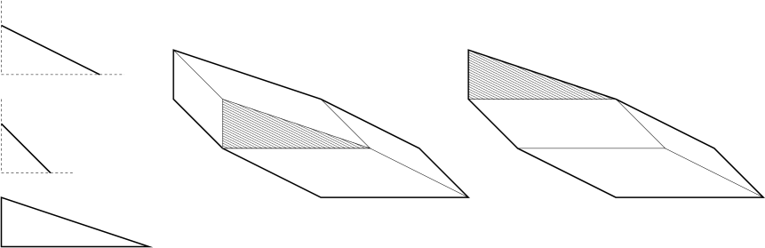
Figure 2: Example 2: polygons $C_{i}$, and two mixed subdivisions of $C$.

Consider segment $L$ defined by vertices $(0,2),(u,2)$ in $C$.

Lemma 9.

The resultant of the $f_{i}\in\mathbb{C}[t,r]$ is homogeneous, of degree $u$, wrt the coefficients of the $a_{i0}$, for $i=0,1,2$.

Proof.

Consider any mixed subdivision of $C$ and the cells of type I and II. Consider these cells as closed polygons: We claim that their union contains segment $L$. Then, it is easy to see that the total volume of these cells equals $u$.

Consider the closed cells that intersect $L$. If the intersection lies in the cell interior, then it is a parallelogram, hence it is mixed and its vertex summand is $(0,1)$, thus it is of type I. If the intersection is a cell edge, say $(a_{kl},a_{km})$, for $k\in\{0,1,2\}$ and $1\leq l<m$, then the cell above $L$ is unmixed, namely a triangle with basis $(a_{kl},a_{km})$ and apex at $(0,3)$. In this case, the cell below $L$ is mixed of type II. ∎

Generically, $u$ equals the total degree of every term in the implicit equation $\phi(x,y)$ wrt $x,y$ and the coefficient of $r$ in $f_{2}$. By prop. 5, the degree of $\Phi(x_{0},x_{1},x_{2})$ is $u$.

In the following, we focus on segment $L$ and subsegments defined by points $(b_{it},2)\in L,i\in\{0,1,2\}$. Usually, we shall omit the ordinate, so the corresponding segments will be denoted by $[b_{jt},b_{kl}]$. We say that such a segment contributes to some coordinate $e_{i}$ when a $i$-mixed cell of the mixed subdivision contains this segment. Moreover,

• a type-I, $i$-mixed cell $a_{i0}+(a_{j0},a_{jt})+(a_{k0},a_{kl})$ is identified with segment $[b_{jt},b_{kl}]$.

• a type-II, $i$-mixed cell $a_{i0}+(a_{jt},a_{js})+(a_{k0},a_{kl})$ is identified with segment $[b_{jt},b_{js}]$ and the coordinate $e_{i}$ to which it contributes.

We show that one needs to examine only subsegments defined by endpoints $b_{iL},b_{iR}\in B_{i}$. This is equivalent to saying that it suffices to consider mixed subdivisions induced by linear liftings.

Theorem 10.

Let $S$ be a mixed subdivision of $C_{0}+C_{1}+C_{2}$, where an internal point $b_{i}\in B_{i}$ defines a 0-dimensional face $(b_{i},2)=(b_{i},0)+(0,1)+(0,1)\in L$. Then, the point of $N(\phi)$ obtained by $S$ cannot be a vertex because it is a convex combination of points obtained by other mixed subdivisions defined by points of $B_{0},B_{1},B_{2}$ which are either endpoints, or are used in defining $S$ except from $(b_{i},2)$.

The theorem is established by lemmas 11, 12 and 13. We shall construct mixed subdivisions that yield points in the $e_{k}e_{j}$-plane whose convex hull contains the initial point. All cells of the original subdivision which are not mentioned are taken to be fixed, therefore we can ignore their contribution to $e_{k},e_{j}$. All convex combinations in these lemmas are decided by the $3\times 3$ orientation determinant (cf. expression (7)).

Lemma 11 (II-II).

Consider the setting of theorem 10 and suppose that $(b_{i},2)$ is a vertex of two adjacent type II cells. Then, the theorem follows.

Proof.

If both cells are $j$-mixed, then the same point in $e_{k}e_{j}$-plane is obtained by one $j$-mixed cell equal to their union, $\{i,j,k\}=\{0,1,2\}$. If the cells are $j$- and $k$-mixed, then there are two mixed subdivisions yielding points in the $e_{k}e_{j}$-plane, which define a segment that contains the initial point. The subdivisions have one $j$-mixed or one $k$-mixed cell respectively, intersecting the entire subsegment. ∎

Lemma 12 (I-I).

Consider the setting of theorem 10 and suppose that $(b_{i},2)$ is a vertex of two adjacent type I cells. Wlog, these are $k$- and $j$-mixed cells, $\{i,j,k\}=\{0,1,2\}$. Then, the theorem follows.

Proof.

Let $[b_{jl},b_{i}],[b_{i},b_{kt}]$ be the subsegments defined on $L$ by the two mixed cells, and let $\alpha,\beta$ be their respective lengths. Since $b_{i}$ is internal, $b_{iR}$ lies to its right-hand side and $b_{iL}$ lies to its left-hand side.

Case $b_{iR}<b_{kt}$ and $b_{iL}>b_{jl}$. Let $\gamma=b_{i}-b_{iL}$ and $\delta=b_{iR}-b_{i}$. The initial point $(\alpha,\beta)$ shall be enclosed by two points. The mixed subdivision with type-I cells corresponding to $[b_{jl},b_{iR}]$ and $[b_{iR},b_{kt}]$ yields point $(\alpha+\delta,\beta-\delta)$. The subdivision with type-I cells corresponding to $[b_{jl},b_{iL}],[b_{iL},b_{kt}]$ yields point $(\alpha-\gamma,\beta+\gamma)$.

Case $b_{iR}<b_{kt}$ and $b_{iL}<b_{jl}$. Let $\gamma=b_{jl}-b_{iL}$ and $\delta=b_{iR}-b_{i}<\beta$. The initial point is $(\alpha+v_{k},\beta+v_{j})$, where $v_{k},v_{j}\geq 0$ is the contribution to $e_{k},e_{j}$ respectively from subsegment $[b_{iL},b_{jl}]$, and $v_{k}+v_{j}\leq\gamma$. Now consider 3 mixed subdivisions on $[b_{iL},b_{kt}]$: The first containing the type-II $k$-mixed cell $[b_{iL},b_{iR}]$ and the type-I $j$-mixed cell $[b_{iR},b_{kt}]$ gives point $(\alpha+\gamma+\delta,\beta-\delta)$. The second containing the type-I $j$-mixed cell $[b_{iL},b_{kt}]$ gives point $(0,\alpha+\beta+\gamma)$. The third containing the type-I $i$-mixed cell $[b_{jl},b_{kt}]$ and the initial cells in $[b_{iL},b_{jl}]$, gives $(v_{k},v_{j})$.

Case $b_{iR}>b_{kt}$ and $b_{iL}>b_{jl}$. Let $\gamma=b_{i}-b_{iL}<\alpha$ and $\delta=b_{iR}-b_{kt}$. The initial point is $(\alpha+v_{k},\beta+v_{j})$, where $v_{k},v_{j}\geq 0$ is the contribution to $e_{k},e_{j}$ respectively from $[b_{kt},b_{iR}]$, and $v_{k}+v_{j}\leq\delta$. Now consider 3 mixed subdivisions on $[b_{jl},b_{iR}]$: The first containing the type-I $i$-mixed cell $[b_{jl},b_{kt}]$ and the initial cells in $[b_{kt},b_{iR}]$, gives point $(v_{k},v_{j})$. The second containing the type-I $k$-mixed cell $[b_{jl},b_{iR}]$, gives point $(\alpha+\beta+\delta,0)$. The third containing the type-I $k$-mixed cell $[b_{jl},b_{iL}]$ and the type-II $j$-mixed cell $[b_{iL},b_{iR}]$, gives $(\alpha-\gamma,\beta+\gamma+\delta)$.

Case $b_{iR}>b_{kt}$ and $b_{iL}<b_{jl}$. Let $\gamma=b_{jl}-b_{iL}$ and $\delta=b_{iR}-b_{kt}$. The initial point is $(\alpha+v_{k}+u_{k},\beta+v_{j}+u_{j})$, where $v_{k},v_{j}\geq 0$ is the contribution to $e_{k},e_{j}$ respectively from $[b_{kt},b_{iR}]$, and $v_{k}+v_{j}\leq\delta$. Similarly, $u_{k},u_{j}\geq 0$ is the contribution to $e_{k},e_{j}$ respectively from $[b_{iL},b_{jl}]$, and $u_{k}+u_{j}\leq\gamma$. Now consider 3 mixed subdivisions on $[b_{iL},b_{iR}]$: The first containing the type-II $k$-mixed cell $[b_{iL},b_{iR}]$, gives point $(\alpha+\beta+\gamma+\delta,0)$. The second containing the type-II $j$-mixed cell $[b_{iL},b_{iR}]$, gives point $(0,\alpha+\beta+\gamma+\delta)$. The third containing the type-I $i$-mixed cell $[b_{jl},b_{kt}]$ and the initial cells in $[b_{iL},b_{jl}]$ and $[b_{kt},b_{iR}]$, gives point $(v_{k}+u_{k},v_{j}+u_{j})$. ∎

\psfrag{S}{\footnotesize$S$}\psfrag{S1}{\footnotesize$S_{1}$}\psfrag{S2}{\footnotesize$S_{2}$}\psfrag{S3}{\footnotesize$S_{3}$}\psfrag{a+g+d}{\footnotesize$\alpha+\gamma+\delta$}\psfrag{u}{\footnotesize$\alpha+\beta+\gamma$}\psfrag{b-d}{\footnotesize$\beta-\delta$}\psfrag{vk}{\footnotesize$v_{k}$}\psfrag{vj}{\footnotesize$v_{j}$}\psfrag{vk,vj}{\footnotesize$v_{k},v_{j}$}\psfrag{a}{\footnotesize$\alpha$}\psfrag{b}{\footnotesize$\beta$}\psfrag{g}{\footnotesize$\gamma$}\psfrag{d}{\footnotesize$\delta$}\psfrag{b+g}{\footnotesize$\beta+\gamma$}\psfrag{a+g}{\footnotesize$\alpha+\gamma$}\psfrag{ek}{\footnotesize$e_{k}$}\psfrag{ej}{\footnotesize$e_{j}$}\psfrag{ei}{\footnotesize$e_{i}$}\psfrag{biL}{\footnotesize$b_{iL}$}\psfrag{bjl}{\footnotesize$b_{jl}$}\psfrag{bi}{\footnotesize$b_{i}$}\psfrag{biR}{\footnotesize$b_{iR}$}\psfrag{bkt}{\footnotesize$b_{kt}$}\includegraphics[width=308.91327pt]{Case2-LI-I.eps}

\psfrag{S}{\footnotesize$S$}\psfrag{S1}{\footnotesize$S_{1}$}\psfrag{S2}{\footnotesize$S_{2}$}\psfrag{S3}{\footnotesize$S_{3}$}\psfrag{a+g+d}{\footnotesize$\alpha+\gamma+\delta$}\psfrag{u}{\footnotesize$\alpha+\beta+\gamma$}\psfrag{b-d}{\footnotesize$\beta-\delta$}\psfrag{vk}{\footnotesize$v_{k}$}\psfrag{vj}{\footnotesize$v_{j}$}\psfrag{vk,vj}{\footnotesize$v_{k},v_{j}$}\psfrag{a}{\footnotesize$\alpha$}\psfrag{b}{\footnotesize$\beta$}\psfrag{g}{\footnotesize$\gamma$}\psfrag{d}{\footnotesize$\delta$}\psfrag{b+g}{\footnotesize$\beta+\gamma$}\psfrag{a+g}{\footnotesize$\alpha+\gamma$}\psfrag{ek}{\footnotesize$e_{k}$}\psfrag{ej}{\footnotesize$e_{j}$}\psfrag{ei}{\footnotesize$e_{i}$}\psfrag{biL}{\footnotesize$b_{iL}$}\psfrag{bjl}{\footnotesize$b_{jl}$}\psfrag{bi}{\footnotesize$b_{i}$}\psfrag{biR}{\footnotesize$b_{iR}$}\psfrag{bkt}{\footnotesize$b_{kt}$}\includegraphics[width=168.49893pt]{Case2-LI-I-subds.eps}

Figure 3: The three points that enclose the point given by $S$ and the corresponding mixed subdivisions for the second case of Lemma 12.

Lemma 13 (I-II).

Consider the setting of theorem 10 and suppose that $(b_{i},2)$ is a vertex of two adjacent type II and I cells. Wlog, these are $k$- and $j$-mixed cells, $\{i,j,k\}=\{0,1,2\}$. Then, the theorem follows.

Proof.

Let $[b_{il},b_{i}],[b_{i},b_{kt}]$ be the subsegments defined on $L$ by the two mixed cells, and let $\alpha,\beta$ be their respective lengths. Since $b_{i}$ is internal, $b_{iR}$ lies to its right-hand side. Moreover, the initial $k$-mixed cell implies the existence of 1-dimensional face $(b_{i},2)+a_{k0}+E_{jl}$, for some edge $E_{jl}=(a_{j0},a_{jl})\subset B_{j}$. The initial $j$-mixed cell implies the existence of 1-face $(b_{i},2)+a_{j0}+E_{kt}$, for edge $E_{kt}=(a_{k0},a_{kt})\subset B_{k}$. The second 1-face cannot be to the left of the first one, hence $b_{jl}\leq b_{kt}$. Hence, $b_{jL}\leq b_{kt}$.

Case $b_{iR}\leq b_{kt}$. The initial point $(\alpha,\beta)$ shall be enclosed by two points. The mixed subdivision with type-I cell $[b_{il},b_{kt}]$ yields point $(0,\alpha+\beta)$. The subdivision with type-II and type-I cells corresponding to $[b_{il},b_{iR}],[b_{iR},b_{kt}]$ sets $e_{k}>\alpha,e_{j}<\beta$, where $e_{k}+e_{j}=\alpha+\beta$.

Case $b_{iR}>b_{kt}$ and $b_{jL}>b_{il}$. Consider subsegment $[b_{il},b_{iR}]$: the initial point is $(\alpha+v_{k},\beta+v_{j})$, where $v_{k},v_{j}\geq 0$ is the contribution to $e_{k},e_{j}$ respectively from subsegment $[b_{kt},b_{iR}]$, and $v_{k}+v_{j}\leq\gamma=b_{iR}-b_{kt}$. Now consider 3 mixed subdivisions on $[b_{il},b_{iR}]$: One $k$-mixed cell $[b_{il},b_{iR}]$ gives point $(\alpha+\beta+\gamma,0)$. One $j$-mixed cell $[b_{il},b_{kt}]$ and the initial cells in $[b_{kt},b_{iR}]$ give $(v_{k},\alpha+\beta+v_{j})$. One $k$-mixed cell $[b_{il},b_{jL}]$, one $i$-mixed cell $[b_{jL},b_{kt}]$ and the initial cells in $[b_{kt},b_{iR}]$ give $(e_{k}+v_{k},v_{j})$, for some $e_{k}\leq\alpha+\beta$.

Case $b_{iR}>b_{kt}$ and $b_{jL}\leq b_{il}$. Consider subsegment $[b_{jL},b_{iR}]$: the initial point is $(\alpha+u_{k}+v_{k},\beta+u_{j}+v_{j})$, where $v_{k},v_{j}$ are as above, $u_{k},u_{j}\geq 0$ correspond to subsegment $[b_{jL},b_{il}]$, and $u_{k}+u_{j}\leq\delta=b_{il}-b_{jL}$. Now consider 3 mixed subdivisions on $[b_{jL},b_{iR}]$: One $k$-mixed cell $[b_{jL},b_{iR}]$ gives point $(\alpha+\beta+\gamma+\delta,0)$. One $j$-mixed cell $[b_{il},b_{iR}]$ and the initial cells in $[b_{jL},b_{il}]$ give $(u_{k},\alpha+\beta+\gamma+u_{j})$. One $i$-mixed cell $[b_{jL},b_{kt}]$, and the initial cells in $[b_{kt},b_{iR}]$ give $(v_{k},v_{j})$. ∎

In the next lemma and corollary, we shall determine certain points in $N(\Phi)$. We shall later see that among these points lie the vertices of $N(\Phi)$ and, therefore, the vertices of $N(\phi)$. Recall that MV${}_{i}=$MV${}_{\mathbb{R}^{2}}(A_{j},A_{k})$, where $\{i,j,k\}=\{0,1,2\}$.

Lemma 14.

Let $b_{tL}=\min\{b_{iL},b_{jL}\},~{}b_{mR}=\max\{b_{iR},b_{jR}\}$ and $\Delta=[b_{tL},b_{mR}]$, for $i\neq j\in\{0,1,2\}$ and $t,m\in\{i,j\}$ not necessarily distinct. Set $e_{\lambda}=|\Delta|$, where $\lambda\in\{0,1,2\}-\{i,j\}$, and $e_{i}=e_{j}=0$. Then, add $b_{tL}$ to $e_{\tau}$, where $\tau\in\{i,j\}-\{t\}$, and add $u-b_{mR}$ to $e_{\mu}$, where $\mu\in\{i,j\}-\{m\}$. Then, $(e_{0},e_{1})$ is a vertex of $N(\phi)$.

Proof.

Clearly $\Delta=$CH$(B_{i}\cup B_{j})\subseteq[0,u]$, so MV${}_{\lambda}=|\Delta|$. It is possible to construct a mixed subdivision that yields the implicit vertex. If $t\neq m$, then the mixed subdivision contains a type-I mixed cell $(a_{t0},a_{tL})+(a_{m0},a_{mR_{m}})+a_{\lambda 0}$ which intersects segment $L$ at subsegment $[b_{tL},b_{mR}]$. This contributes $\mbox{\rm MV}_{\lambda}=b_{mR}-b_{tL}$ to $e_{\lambda}$. There is a type-I cell $(a_{\lambda 0},a_{\lambda L})+(a_{t0},a_{tL})+a_{\tau 0}$ which intersects $L$ at subsegment $[0,b_{tL}]$. This contributes $b_{tL}$ to $e_{\tau}$. Similarly, we assign the area $u-b_{mR}$ of the type-I cell $(a_{\lambda 0},a_{\lambda R})+(a_{m0},a_{mR_{m}})+a_{\mu 0}$ to $e_{\mu}$.

If $t=m$, then $\Delta$ is an edge of one of the initial Newton segments, say $B_{t}$, and $\Delta=[b_{tL},b_{tR}]$. The mixed subdivision contains the type-II mixed cell $(a_{\tau 0},a_{\tau L})+(a_{tL},a_{tR})+a_{\lambda 0}$ which contributes $\mbox{\rm MV}_{\lambda}=|\Delta|=b_{tR}-b_{tL}$ to $e_{\lambda}$. There are also two type-I cells intersecting $L$ at its leftmost and rightmost subsegments, as in the previous case. Since $t=m$, we have $\mu=\tau$, hence $e_{t}=0$.

The type-I mixed cells in any of the above mixed subdivisions vanish when $b_{tL}=0$ or $b_{mR}=u$. Notice that $e_{i}+e_{j}+e_{\lambda}=u$ and since $e_{\lambda}$ is maximized, $(e_{0},e_{1},e_{2})$ defines a vertex of $N(\Phi)\subset\mathbb{R}^{3}$. Projecting to the $e_{0}e_{1}$-plane yields the implicit vertex.

\psfrag{Al}{\footnotesize$A_{\lambda}$}\psfrag{Ai}{\footnotesize$A_{i}$}\psfrag{Aj}{\footnotesize$A_{j}$}\psfrag{t=m=j}{\footnotesize$t=m=j$}\psfrag{tn=m}{\footnotesize$i=t\neq m=j$}\includegraphics[width=505.48822pt]{L419-mxd-subds.eps}

Figure 4: Lemma 14: the mixed subdivisions for the cases $t=m$ and $t\neq m$.

∎

The following corollary is proven similarly to the above proof.

Corollary 15.

Under the notation of lemma 14 consider the following 3 definitions:

1. $b_{tL}=\min\{b_{iL},b_{jL}\},~{}b_{mR}=\min\{b_{iR},b_{jR}\}$,

2. $b_{tL}=\max\{b_{iL},b_{jL}\},~{}b_{mR}=\max\{b_{iR},b_{jR}\}$,

3. $b_{tL}=\max\{b_{iL},b_{jL}\},~{}b_{mR}=\min\{b_{iR},b_{jR}\}$, provided $b_{tL}\leq b_{mR}$.

In each case, define $e_{0},e_{1},e_{2}$ as in lemma 14. Then $(e_{0},e_{1})\in N(\phi)$.

3.1 The implicit vertices

Overall, there are three cases for the relative positions of the $B_{i}$:

1. CH$(B_{i}\cup B_{j})=[0,u]$ for all pairs $i,j$.

2. CH$(B_{j}\cup B_{l})=$ CH$(B_{i}\cup B_{l})=[0,u]\neq$ CH$(B_{i}\cup B_{j})$.

3. CH$(B_{i}\cup B_{j})=[0,u]\neq$ CH$(B_{l}\cup B_{t})$ for $t=i,j$.

Orthogonally, we can distinguish the following two cases:
(A) there exists at least one $B_{i}=[0,u]$,
(B) none of the $B_{i}$’s equals $[0,u]$.

In case (B), every union $B_{i}\cup B_{j}$ contains either 0 or $u$. Cases (1B) and (3A) cannot exist, which leaves 4 cases overall. In the sequel, we let $E_{it}$ denote a segment $(a_{i0},a_{it})\subset B_{i}$.

Theorem 16 (case (A)).

If all unions CH$(B_{i}\cup B_{j})=[0,u],i\neq j$, then the implicit polygon is a triangle with vertices $(0,0),(0,u),(u,0)$. If exactly one support, say $B_{k},k\in\{0,1,2\}$, equals $[0,u]$, then $N(\phi)$ has up to 5 vertices in the following set of $(e_{i},e_{j})$ vectors:

$$\{(u,0),(0,u),(0,u-b_{iR}+b_{iL}),(b_{jL},u-b_{iR}),(u-b_{jR}+b_{jL},0)\},$$

where $\{i,j,k\}=\{0,1,2\}$, assuming $i,j$ are chosen so that

$$b_{iL}(u-b_{jR})\geq b_{jL}(u-b_{iR}).$$ (6)

\psfrag{ei}{$e_{i}$}\psfrag{ej}{$e_{j}$}\psfrag{e2}{$e_{k}$}\psfrag{biL}{$b_{iL}$}\psfrag{bjL}{$b_{jL}$}\psfrag{biR}{$b_{iR}$}\psfrag{bjR}{$b_{jR}$}\psfrag{u}{$u$}\psfrag{u_biR}{$u-b_{iR}$}\psfrag{u_Bi}{$u-b_{iR}+b_{iL}$}\psfrag{u_Bj}{$u-b_{jR}+b_{jL}$}\includegraphics[width=308.91327pt]{case2a.eps}

Figure 5: The implicit polygon in case (2A), in the $e_{i}e_{j}$-plane, and the subdivisions of the proof of theorem 16.

Proof.

First is the case (1A), established from lemma 14. The second statement concerns case (2A): By switching $i$ and $j$, assumption (6) can always be satisfied. Unless $B_{i}\subset B_{j}$ or $B_{j}\subset B_{i}$, this assumption holds simply by choosing $i,j$ so that $b_{jL}\leq b_{iL}$.

The vertices $(u,0),(0,u)$ are obtained by lemma 14, applied to CH$(B_{j}\cup B_{k})$ and CH$(B_{i}\cup B_{k})$ respectively. The third point is obtained by a mixed subdivision with two type-I cells $E_{iL}+a_{j0}+E_{kL},E_{iR}+a_{j0}+E_{kR}$, which contribute the lengths of $[b_{kL},b_{iL}],[b_{iR},b_{kR}]$ to $e_{j}$, and one type-II cell $E_{i0}+E_{jt}+a_{k0}$, contributing the length of $[b_{iL},b_{iR}]$ to $e_{k}$, where $E_{i0}$ is the horizontal edge of $A_{i}$ and $t\in\{L,R\}$; see figure 5. By switching $i$ and $j$ we define a subdivision that yields the fifth point.

The fourth point is obtained by a subdivision with 3 type-I cells: $a_{i0}+E_{jL}+E_{kL},E_{iR}+a_{j0}+E_{kR}$ and $E_{iR}+E_{jL}+a_{k0}$, which contribute to $e_{i},e_{j}$ and $e_{k}$ respectively, see fig. 5. It suffices to show that the line defined by this and the third point supports the implicit polygon. An analogous proof then shows that the line defined by this and the 5th point also supports the polygon, and the theorem follows. Our claim is equivalent to showing

$$\det\left[\begin{array}[]{ccc}b_{jR}&u-b_{iR}&1\\ 0&u-b_{iR}+b_{iL}&1\\ e_{i}&e_{j}&1\end{array}\right]\leq 0\Leftrightarrow b_{iL}(e_{i}-b_{jL})\geq b_{jL}(u-b_{iR}-e_{j}).$$ (7)

We consider the rightmost subsegment on $L$, where one endpoint is $b_{kR}=u$. This contributes to either $e_{i}$ or $e_{j}$ an amount equal to the length of a subsegment extending at least as far left as $b_{jR}$ or $b_{iR}$, respectively. Symmetrically, the leftmost subsegment has endpoint $b_{kL}=0$ and contributes to $e_{i}$ or $e_{j}$ the length of a subsegment extending at least as far right as $b_{jL}$ or $b_{iL}$, respectively. In general, there are 4 cases, depending on the contribution of the rightmost and leftmost subsegments. The last case is infeasible if $B_{i},B_{j}$ have no overlap.

If the rightmost subsegment contributes to $e_{j}$ then $e_{j}\geq u-b_{iR}$. If the leftmost subsegment contributes to $e_{j}$ then this contribution is at least $b_{iL}$, hence $e_{j}\geq u-b_{iR}+b_{iL}$, where $e_{i}\geq 0$. Otherwise, the leftmost subsegment contributes to $e_{i}$, thus $e_{i}\geq b_{jL}$. In both cases, inequality (7) follows.

If the rightmost subsegment contributes to $e_{i}$ then $e_{i}\geq u-b_{jR}$. If the leftmost subsegment also contributes to $e_{i}$, then $e_{i}\geq u-b_{jR}+b_{jL}$. Using also $e_{j}\geq 0$, it suffices to prove $b_{iL}(u-b_{jR})\geq b_{jL}(u-b_{iR})$. Otherwise, the leftmost subsegment contributes to $e_{j}$, so $e_{j}\geq b_{iL}$, and it suffices to prove $b_{iL}(u-b_{jR}-b_{jL})\geq b_{jL}(u-b_{iR}-b_{iL})$. Both sufficient conditions are equivalent to assumption (6). ∎

Theorem 17 (case (B)).

If none of the $B_{t}$’s is equal to $[0,u]$, then we may choose $\{i,j,k\}=\{0,1,2\}$ such that:

$$0<b_{iL}\leq b_{iR}=u,0=b_{jL}\leq b_{jR}<u,0\leq b_{kL}\leq b_{kR}<u.$$

Then, $N(\phi)$ has at most 5 or 4 vertices, depending on whether $b_{kL}$ is positive or 0. In the former case, the vertices $(e_{i},e_{j})$ lie in

$$\{(b_{jR},0),(b_{kR},u-b_{kR}),(b_{kL},u-b_{kL}),(0,u-b_{0L}),(0,0),\}$$

and, in the latter case, the third and fourth vertices are replaced by $(0,u)$.

By lemma 9, at every point $e_{k}=u-e_{i}-e_{j}$. The theorem is established by the following two lemmas.

Lemma 18 (case (2B)).

Suppose $b_{kL}=0$ in theorem 17 and wlog assume $b_{jR}\leq b_{kR}$. Then, $N(\phi)$ has up to 4 vertices $(e_{i},e_{j})$ in the set

$$\{(b_{jR},0),(b_{kR},u-b_{kR}),(0,u),(0,0)\}.$$

Proof.

The last two vertices follow from lemma 14, applied to CH$(B_{i}\cup B_{k})$ and CH$(B_{i}\cup B_{j})$, respectively. The same lemma, applied to CH$(B_{j}\cup B_{k})$, yields the second vertex, whereas cor. 15(1) yields the first point. It suffices to show that any point $(e_{i},e_{j})\in N(\phi)$ defines a counter-clockwise turn in the $e_{i}e_{j}$-plane, when appended to $(b_{jR},0)$ and $(b_{kR},u-b_{kR})$. This is equivalent to proving

$$\det\left[\begin{array}[]{ccc}b_{jR}&0&1\\ b_{kR}&u-b_{kR}&1\\ e_{i}&e_{j}&1\end{array}\right]\geq 0\Leftrightarrow e_{j}(b_{kR}-b_{jR})\geq(u-b_{kR})(e_{i}-b_{jR}).$$ (8)

Rightmost segment $[b_{kR},b_{iR}=u]$ cannot contribute to $e_{i}$, since each corresponding mixed cell has an edge summand from $A_{i}$. If the segment lies in a $j$-mixed cell, then $e_{j}\geq u-b_{kR}$ and $e_{i}\leq b_{kR}$, and inequality (8) is proven. Otherwise, at least a subsegment contributes to a $k$-mixed cell.

If this subsegment contains $b_{kR}$, then it must extend at least to the next endpoint lying left of $b_{kR}$, hence to $b_{jR}$ or $b_{iL}$. In the latter case, the subsegment to the left of $b_{iL}$ cannot contribute to $e_{i}$. Thus, in any case, $e_{i}\leq b_{jR}$, so (8) is proven.

If none of the above happens, then the subsegment contributing to $e_{k}$ does not contain $b_{kR}$, so the only way for the $k$-mixed cell to be defined is to have $b_{iL}$ lie in $(b_{kR},b_{iR})$ and $k$-mixed cell intersecting $L$ at $[b_{iL},b_{iR}]$. Then, $[b_{kR},b_{iL}]$ contributes to $e_{j}$, so the $j$-mixed cell intersects $L$ at $[b_{kt},b_{iL}]$, where $t\in\{L,R\}$. If $b_{kt}=b_{kL}$, then $e_{i}=0$ and (8) is proven.

Otherwise, $b_{kt}=b_{kR}$. The $j$-mixed cell is of type I and implies that the $1$-dimensional face $(b_{iL},2)+E_{kR}$ belongs to the subdivision, see lemma 8. The $k$-mixed cell is of type II, with some edge summand $E_{jt}\subset A_{j}$, which implies that the $1$-face $(b_{iL},2)+E_{jt}$ is in the subdivision and cannot lie to the left of the previous $1$-face. Since $b_{jR}\leq b_{kR}$, we have $b_{kR}=b_{jR}$, hence $e_{i}\leq b_{jR}$. ∎

Lemma 19 (case (3B)).

Suppose $b_{kL}>0$ in theorem 17. Then, $N(\phi)$ has up to 5 vertices $(e_{i},e_{j})$ in the set

$$\{(b_{jR},0),(b_{kR},u-b_{kR}),(b_{kL},u-b_{kL}),(0,u-b_{iL}),(0,0)\}.$$

Proof.

The last vertex follows from lemma 14, applied to CH$(B_{i}\cup B_{j})$. We shall prove that the first two points are vertices; they are obtained by using CH$(B_{j}\cup B_{k})$ in lemma 14 and cor. 15(1). Which point is obtained from which lemma depends on the sign of $b_{jL}-b_{kL}$. The third and fourth vertices are established analogously, by considering CH$(B_{i}\cup B_{k})$.

Our proof shall establish inequality (8). If $b_{jR}\leq b_{kR}$, this is similar to the proof of lemma 18. Otherwise, $b_{kR}<b_{jR}$, and the rightmost segment $[b_{jR},b_{iR}=u]$ cannot contribute to $e_{i}$. If it contributes to $e_{k}$ only, then $e_{k}\geq u-b_{jR}$ so $e_{i}+e_{j}\leq b_{jR}$ and (8) follows.

If it contributes to $e_{j}$ only, the union of the corresponding $j$-mixed cells intersect $L$ at a segment with an endpoint to the left of $b_{jR}$, namely $b_{kt},t\in\{L,R\}$, or $b_{iL}$. In the former case, $e_{i}\leq b_{kR}$ and $e_{j}\geq u-b_{kR}$. In the latter case, $[0,b_{iL}]$ contributes to $e_{k}$ only, so $e_{i}=0,e_{j}=u-b_{iL}$. In both cases, (8) follows readily.

Lastly, $[b_{jR},b_{iR}]$ might be split into subsegments $[b_{jR},b_{iL}],[b_{iL},b_{iR}]$, contributing to $e_{k},e_{j}$ respectively. The corresponding cells are of type I and type II, the latter having an edge summand from $A_{k}$. This requires the subdivision to have $j$-faces $(b_{iL},k)+E_{jR}$ and $(b_{iL},2)+E_{kt},t\in\{L,R\}$, where the first lies to the left of the second, see lemma 8. This cannot happen because $b_{kR}<b_{jR}$. ∎

Example 3.

For the unit circle,

$$x=2t/(t^{2}+1),~{}y=(1-t^{2})/(t^{2}+1)$$

we have $f_{0}=xt^{2}-2t+x,~{}f_{1}=(y+1)t^{2}+(y-1)$. In lemma 14, the sets $B_{0}=\{1\},B_{1}=\{0,2\},B_{2}=\{0,2\}$ yield terms $x^{2},y^{2},1$ in $\phi$ and, hence, an optimal support. See example 13 for a treatment assuming different denominators.

Example 4.

For the folium of Descartes

$$x=\frac{3t^{2}}{t^{3}+1},y=\frac{3t}{t^{3}+1}\Rightarrow\phi=x^{3}+y^{3}-3xy=0;$$

see example 2 and figure 2. Now, $B_{0}=\{2\},B_{1}=\{1\},B_{2}=\{0,3\}$, hence this is case (2B). In theorem 16, we set $i=0,j=1,k=2$ and obtain, in the order stated by the theorem: $x^{3},x^{3},y^{3},y^{3},xy$, hence an optimal support.

If we do not account for the same denominators, use degree bounds alone, or project the Sylvester resultant, we obtain an overestimation of the support.

Example 5.

$$x=\frac{2t^{3}+t+1}{t^{2}+1},y=\frac{t^{4}+t^{3}-1}{t^{2}+1},$$

hence $B_{0}=\{0,1,3\},B_{1}=\{0,3,4\},B_{2}=\{0,2\}$, so this is case (2A) with $B_{1}=[0,u]$. In theorem 16, we set $i=0,j=2$ and obtain the vectors $(e_{i},e_{j})=(4,0),(0,4),(0,1),(0,3),(2,0)$, in the order stated by the theorem. This yields the implicit points $(e_{0},e_{1})=(4,0),(0,0),(0,3),(0,1),(2,2)$, hence vertices $(4,0),(0,0),(0,3),(2,2)$. These define the optimal polygon because the implicit equation is

$$\phi=59-21x+110y+52y^{2}-13x^{2}-48xy+5x^{3}-5x^{2}y-x^{4}+8y^{3}-2x^{2}y^{2}+2x^{3}y-12xy^{2}.$$

If we do not exploit the identical denominators, we obtain a superset of the support.

Example 6.

$$x=\frac{t^{6}+2t^{2}}{t^{7}+1},y=\frac{t^{4}-t^{3}}{t^{7}+1},$$

hence $B_{0}=\{2,6\},B_{1}=\{3,4\},B_{2}=\{0,7\}$, so this is case (2A) with $B_{2}=[0,u]$. In theorem 16, we set $i=0,j=1$ and obtain the implicit points $(e_{0},e_{1})=(7,0),(0,7),(0,3),(3,1),(6,0)$, in the order stated by the theorem. These are also the implicit vertices and define the optimal polygon because the implicit equation is

$\phi=-32y^{4}-30x^{3}y^{2}-x^{4}y-12x^{2}y^{2}-3x^{3}y-7x^{6}y-2x^{7}+20xy^{3}+280x^{2}y^{5}-7^{3}y^{4}x-70x^{4}y^{3}-\\ 22x^{3}y^{3}-49x^{5}y^{2}-21x^{4}y^{2}+11x^{5}y+216y^{5}+129y^{7}-248y^{6}+70xy^{6}+185xy^{5}+24y^{3}+100xy^{4}+\\ 43x^{2}y^{3}+72x^{2}y^{4}+3x^{6}.\\$

In figure 1 is shown the implicit polygon. Changing the coefficient of $t^{2}$ to -1, leads to an implicit polygon with 6 vertices $(1,3),(0,4),(0,6),(2,5),(7,0),(4,1)$, which is contained in the polygon predicted by theorem 16. This shows the importance of the genericity condition on the coefficients of the parametric polynomials.

4 Polynomial parameterizations

We consider polynomial parameterizations of curves. In this case we define polynomials

$$f_{0}=x-P_{0}(t),~{}f_{1}=y-P_{1}(t)\in(\mathbb{C}[x,y])[t].$$

The supports of $f_{0},f_{1}$ are fixed, namely $A_{0}=\{a_{00},a_{01},\ldots,a_{0n}\}$ and $A_{1}=\{a_{10},a_{11},\ldots,a_{1m}\}$, with generic coefficients. Here, $a_{0i}$ and $a_{1j}$ are sorted in ascending order. Points $a_{00},a_{10}$ are always equal to zero. The new point set

$$C=\kappa(A_{0},A_{1})=\{(a_{00},0),\ldots,(a_{0n},0),(a_{10},1),\ldots,(a_{1m},1)\},\in\mathbb{N}^{2}$$

is introduced by the Cayley embedding. For convenience, we shall omit the second coordinate. Every triangulation of this set is regular, and corresponds to a mixed cell configuration of $A_{0}+A_{1}$.

The resultant $\mathcal{R}(f_{0},f_{1})$ is a polynomial in $x,y,c_{ij}$, where $c_{ij}$ are the coefficients of the polynomials $P_{i}$. We consider the specialization of coefficients $c_{ij}$ in the resultant. Generically, this specialization yields the implicit equation. Now, $N(\phi)\subset\mathbb{Z}^{2}$ with vertices obtained from those extreme monomials of $\mathcal{R}(f_{0},f_{1})$ which contain coefficients of $a_{00}$ and $a_{10}$. Since every triangle of a triangulation $T$ of $C$ corresponds to a mixed cell of a mixed subdivision of $A_{0}+A_{1}$, we can rewrite relation (1) as:

$$\pm\prod_{i=0}^{1}\prod_{R}c_{i,p}^{\mathrm{Vol}(R)},$$ (9)

where $R$ is an $i$-mixed cell with vertex $p\in A_{i}$ and $c_{i,p}$ is the coefficient of the monomial with exponent $p\in A_{i}$. After specialization of the coefficients of $f_{0},f_{1}$, the terms of (9) associated with mixed cells having a vertex $p$ other than $a_{00},a_{10}$ contribute only a constant to the corresponding term. This implies that the only mixed cells that we need to consider are the ones with vertex $a_{00}$ or $a_{10}$ (or both). For any triangulation $T$, these mixed cells correspond to triangles with vertices $a_{00},a_{1l},a_{1r}$ where $l,r\in\{0,\dots,m\}$, or $a_{10},a_{0l},a_{0r}$, where $l,r\in\{0,\dots,n\}$.

The first statement below can be obtained from the degree bounds; we establish it by our methods for completeness.

Theorem 20.

If $P_{0}$ or $P_{1}$ (or both) contain a constant term, then the implicit polygon is the triangle with vertices $(0,0),(a_{1m},0),(0,a_{0n})$. Otherwise, $P_{0},P_{1}$ contain no constant terms, and the implicit polygon is the quadrilateral with vertices $(a_{11},0),(a_{1m},0)$, $(0,a_{0n}),(0,a_{01})$.

Proof.

Let us consider the first statement. To obtain vertices $(a_{1m},0)$ and $(0,0)$ consider the triangulation $T$ of $C$ obtained by drawing edge $(a_{00},a_{1m})$ (see figure 6). The only 0-mixed cell with vertex $a_{00}$ corresponding to $T$ is $R=a_{00}+(a_{10},a_{1m})$ with volume equal to $a_{1m}$; there are no 1-mixed cells with vertex $a_{10}$. The extreme monomial associated with such a triangulation is of the form $(x-c_{00})^{a_{1m}}c_{1m}^{a_{0n}}$ which, after specializing $c_{00},c_{1m}$ and expanding, gives monomials in $x$ with exponents $a_{1m},a_{1m-1},\ldots,0$.

For vertex $(0,a_{0n})$ consider triangulation $T^{\prime}$ obtained by drawing edge $(a_{10},a_{0n})$. The only 1-mixed cell with vertex $a_{10}$ is $R=a_{10}+(a_{00},a_{0n})$ with volume equal to $a_{0n}$; there are no 0-mixed cells with vertex $a_{00}$. The extreme monomial is $(y-c_{10})^{a_{0n}}c_{0n}^{a_{1m}}$ which, after specializing $c_{10},c_{0n}$ and expanding, gives monomials in $y$ with exponents $a_{0n},a_{0n-1},\ldots,0$.

To complete the proof it suffices to observe that every triangulation of $C$ having edges of the form $(a_{00},a_{1j}),~{}0<j<m$ and $(a_{1j},a_{0i})$, $i>0$ leads to an extreme monomial which specializes to a polynomial in $x$ of degree $a_{1j}$. Therefore we obtain monomials with exponents $(a_{1j},0),\ldots,(0,0)$ which lie in the interior of the triangle. Similarly, every triangulation of $C$ having edges of the form $(a_{10},a_{0i}),~{}0<i<n$ and $(a_{0i},_{1j})$, $j>0$ leads to an extreme monomial which specializes to a polynomial in $y$ of degree $a_{0i}$. Therefore we obtain monomials with exponents $(0,a_{0i}),\ldots,(0,0)$ which lie in the interior of the triangle.

The extreme monomials associated with $a_{00}$ and $a_{10}$ are specialized to monomials of the implicit equation in $x$ or $y$ respectively, thus not producing any constant terms. The proof of the previous lemma implies that, when $y$’s exponent is $0$, the smallest exponent of $x$ is $a_{11}$, which is obtained by a triangulation containing edges $(a_{00},a_{11})$ and $(a_{11},a_{0i}),~{}i>0$. Similarly, the smallest exponent of $y$ is $a_{01}$. ∎

\psfrag{a0}{\tiny$a_{00}$}\psfrag{a1}{\tiny$a_{01}$}\psfrag{an}{\tiny$a_{0n}$}\psfrag{b0}{\tiny$a_{10}$}\psfrag{b1}{\tiny$a_{11}$}\psfrag{bm}{\tiny$a_{1m}$}\psfrag{YM}{\tiny$(0,a_{0n})$}\psfrag{Ym}{\tiny$(0,a_{01})$}\psfrag{XM}{\tiny$(a_{1m},0)$}\psfrag{Xm}{\tiny$(a_{11},0)$}\includegraphics[width=336.99786pt]{Nf_polynomial.eps}

Figure 6: The implicit polygon of a polynomially parameterized curve.

Now we use [GKZ90, Prop.15] to arrive at the following; recall that the implicit equation is defined up to a sign. The coefficient of $x^{a_{1m}}$ is $c(-1)^{(1+a_{0n})a_{1m}}c_{1m}^{a_{0n}}$ and that of $y^{a_{0n}}$ is $c(-1)^{a_{0n}(1+a_{1m})}c_{0n}^{a_{1m}}$, where $c\in\{-1,1\}$.

Corollary 21.

There exists $c\in\{-1,1\}$ s.t. the coefficient of $x^{a_{1m}}$ is $c(-c_{1m})^{a_{0n}}$ and that of $y^{a_{0n}}$ is $c(-c_{0n})^{a_{1m}}$.

Example 7.

Parameterization $x=y=t$ yields implicit equation $\phi=x-y$. Our method yields vertices $(1,0)$ and $(0,1)$ which are optimal.

Example 8.

Parameterization $x=2t^{3}-t+1,y=t^{4}-2t^{2}+3$ yields implicit equation $\phi=608-136x+569y+168y^{2}-72x^{2}-32xy-4x^{3}-16x^{2}y-x^{4}+16y^{3}$. Our method yields the vertices $(0,0),(4,0),(0,3)$ which are optimal. The degree bounds describe a larger quadrilateral with vertices $(0,0),(4,0),(1,3),(0,3)$. Corollary 21 predicts, for $x^{4}$, coefficient $(-1)^{16}=1$, and for $y^{3}$, coefficient $(-1)^{15}2^{4}=-16$, up to a fixed sign which equals $-1$ in $\phi(x,y)$.

Example 9.

For the Fröberg-Dickenstein example [EK05, Exam.3.3],

$$x=t^{48}-t^{56}-t^{60}-t^{62}-t^{63},y=t^{32},$$

our method yields vertices $(32,0),(0,48),(0,63)$, which define the optimal polygon. Here the degree bounds describe the larger quadrilateral with vertices $(0,0),(32,0),(32,31),(0,63)$.

Example 10.

Parameterization $x=t+t^{2},y=2t-t^{2}$ yields implicit equation $\phi=6x-3y+x^{2}+2xy+y^{2}$. The previous lemma yields vertices $(1,0),(2,0),(0,2),(0,1)$, which define the actual implicit polygon. Here the degree bounds imply a larger triangle, with vertices $(0,0),(2,0),(0,2)$. Corollary 21 predicts, for $x^{2}$ and $y^{2}$, coefficients $(-1)^{6}(-1)^{2}=1$ and $(-1)^{6}(1)^{2}=1$ respectively.

5 Rational parameterizations with different denominators

Now we turn to the case of rationally parameterized curves, with different denominators. We have

$$f_{0}(t)=xQ_{0}(t)-P_{0}(t),\ f_{1}(t)=yQ_{1}(t)-P_{1}(t)\ \in(\mathbb{C}[x,y])[t],\,\gcd(P_{i},Q_{i})=1,$$

and let $c_{ij}~{}(0\leq j\leq m_{i})$,  $q_{ij}~{}(0\leq j\leq k)$ denote the coefficients of polynomials $P_{i}(\mathrm{t})$ and $Q_{i}(t)$, respectively. The supports of $f_{0},f_{1}$ are of the form $A_{0}=\{a_{00},a_{01},\ldots,a_{0n}\}$ and $A_{1}=\{a_{10},a_{11},\ldots,a_{1m}\}$ where the $a_{0i}$ and $a_{1j}$ are sorted in ascending order; $a_{00}=a_{10}=0$ because $\gcd(P_{i},Q_{i})=1$. Points in $A_{0},A_{1}$ are embedded by $\kappa$ in $\mathbb{R}^{2}$. The embedded points are denoted by $(a_{0i},0),(a_{1i},1)$; by abusing notation, we will omit the extra coordinate.

Recall that each $p\in A_{0}$ corresponds to a monomial of $f_{0}$. The corresponding coefficient either lies in $\mathbb{C}$, or is a monomial $q_{i}x$, or a binomial $q_{i}x+c_{0i}$, where $q_{i},c_{0i}\in\mathbb{C}$. An analogous description holds for the second polynomial.

Definition 3.

Let $V,W$ be non-empty subsets of $\mathbb{Z}$. A selection is a pair of sets $S,T$ such that $S\subseteq V$ and $T\subseteq W$. We say that the elements of the sets $S$ and $T$ are selected, and that the elements of $V\setminus S$ and $W\setminus T$ are non-selected.

With respect to the sets $A_{0}$ and $A_{1}$, we now define two types of selections:

• Selection1: the exponents in $A_{0}$ and $A_{1}$ corresponding to coefficients which are non-constant polynomials (i.e., they are either linear monomials or linear binomials) in $\mathbb{C}[x]$ and $\mathbb{C}[y]$, respectively, are selected. Let $S_{i}\subseteq A_{i}$ ($i=0,1$) be the sets of the selection. The selected exponents in $S_{i}$ are those in the support of the denominator $Q_{i}(t)$; moreover, $|S_{0}|\geq 1$ and $|S_{1}|\geq 1$, i.e., at least one exponent from both $A_{0}$ and $A_{1}$ is selected since $Q_{i}(t)\neq 0$.

• Selection2: the exponents in $A_{0}$ and $A_{1}$ corresponding to coefficients which are monomials in $\mathbb{C}[x]$ and $\mathbb{C}[y]$, respectively, are selected. Let $S^{\prime}_{i}\subseteq A_{i}$ ($i=0,1$) be the sets of the selection. In this case, $S^{\prime}_{i}={\rm supp}(Q_{i})\setminus{\rm supp}(P_{i})$; there is at least one non-selected exponent in $A_{0}$ and in $A_{1}$ coming from the numerator $P_{i}(t)$.

In order to denote that $a_{0i}\in A_{0}$ or $a_{1i}\in A_{1}$ is selected (non-selected, resp.), we write $a_{0i}^{+}$ or $a_{1i}^{+}$  ($a_{0i}^{-}$ or $a_{1i}^{-}$, resp.). For example, the case of polynomial parameterizations yields $A_{0}=\{a_{00}^{+},a_{01}^{-},\dots,a_{0n}^{-}\}$, $A_{1}=\{a_{10}^{+},a_{11}^{-},\dots,a_{1m}^{-}\}$, under Selection1.

We shall consider only $i$-mixed cells associated with a selected vertex in $A_{i}$. For any triangulation $T$, these mixed cells correspond either to triangles with vertices $\{a_{0i}^{+},a_{1{\ell}},a_{1r}\}$, where ${\ell},r\in\{0,\dots,m\}$, or to $\{a_{0{\ell}},a_{0r},a_{1j}^{+}\}$, where ${\ell},r\in\{0,\dots,n\}$. Given a selection and a triangulation, we set

$$e_{0}=\sum_{i,\ell,r}{\rm Vol}(a_{0i}^{+},a_{1{\ell}},a_{1r}),\qquad\qquad e_{1}=\sum_{\ell,r,j}{\rm Vol}(a_{0{\ell}},a_{0r},a_{1j}^{+}),$$ (10)

where $i,j$ range over all selected points in $A_{0}$ and $A_{1}$, respectively, and we sum up the normalized volumes of mixed triangles.

In the following, we use the upper (lower, resp.) hull of a convex polygon in $\mathbb{R}^{2}$ wrt some direction $v\in\mathbb{R}^{2}$. Let us consider the unbounded convex polygons defined by the computed upper and lower hulls. The intersection of these two unbounded polygons is the implicit Newton polygon.

The resultant $\mathcal{R}(f_{0},f_{1})$ is a polynomial in $x,y,c_{ij},q_{k}$. We consider the specialization of coefficients $c_{ij},q_{k}$ in order to study $\phi$; this specialization yields the implicit equation. The relevant terms are products of one polynomial in $x$ and one in $y$. The former is the product of powers of terms of the form $q_{i}x$ or $q_{i}x+c_{0j}$ ; the $y$-polynomial is obtained analogously.

Lemma 22.

Consider all points $(e_{0},e_{1})$ defined by expressions (10). The polygon defined by the upper hull of points $(e_{0},e_{1})$ under Selection1 and the lower hull of points $(e_{0},e_{1})$ under Selection2 equals the implicit polygon $N(\phi)$.

Proof.

Consider the extreme terms of the resultant, given by thm 2 and expression (9). After the specialization of the coefficients, those associated with $i$-mixed cells having a non-selected vertex $p\in A_{i}$ contribute only a coefficient in $\mathbb{C}$ to the corresponding term of $\phi$. This is why they are not taken into account in (10).

Now consider Selection1. By maximizing $e_{0}$ or $e_{1}$, as defined in (10), it is clear that we shall obtain the maximum possible exponents in the terms which are polynomials in $x$ and $y$ respectively, hence the largest degrees in $x,y$ in $\phi$. Under certain genericity assumptions, we shall obtain all vertices in the implicit polygon, which appear in its upper hull with respect to vector $(1,1)$. If genericity fails, the implicit polygon will contain vertices with smaller coordinates.

Selection2 minimizes the powers of coefficients corresponding to monomials in the implicit variables. All other coefficients are in $\mathbb{C}$ or are binomials in $x$ (or $y$), so they contain a constant term, hence their product will contain a constant, assuming generic coefficients in the parametric equations. Therefore these are vertices on the lower hull with respect to $(1,1)$. If genericity fails, then fewer terms appear in $\phi$ and the implicit polygon is interior to the lower hull computed. ∎

5.1 The implicit vertices

For a set $P$ and any $p\in P$, we define functions $\mathcal{X}(p^{+})$ and $\mathcal{X}(P^{-})$ where $\mathcal{X}(p^{+})=1$ if $p$ is selected and $\mathcal{X}(p^{+})=0$ otherwise, and $\mathcal{X}(P^{-})=1$ if there exists some non-selected point $p^{-}\in P$ and $\mathcal{X}(P^{-})=0$ otherwise. Function $\mathcal{X}(P^{-})$ satisfies ${\mathcal{X}}(P^{-})=1-\prod_{i}{\mathcal{X}}(p_{i}^{+})$. Recall that $a_{00}=a_{10}=0$; nevertheless, we still use $a_{00},a_{10}$ for generality.

The following two lemmas describe the upper hull defined by expressions (10).

Lemma 23.

The maximum exponent of $x$ in the implicit equation is $e_{0}^{max}=a_{1m}-a_{10}.$ When this is attained, the maximum exponent of $y$ is

$$e_{1}^{max}|_{e_{0}^{max}}=(a_{0R}^{+}-a_{0L}^{+})+\mathcal{X}(a_{10}^{+})\cdot(a_{0L}^{+}-a_{00})+\mathcal{X}(a_{1m}^{+})\cdot(a_{0n}-a_{0R}^{+}),$$

where $a_{0R}^{+},a_{0L}^{+}$ are the rightmost and leftmost selected points (not necessarily distinct) in $A_{0}$, with respect to Selection1. A symmetric result holds for $e_{0}^{max}|_{e_{1}^{max}}$.

Proof.

There always is at least one selected point $a_{0j}^{+}\in A_{0}$ and $a_{1i}^{+}\in A_{1}$. This implies that the maximum exponent of $x$ is equal to $a_{1m}-a_{10}$ and is attained by the triangulation with edges $(a_{0j}^{+},a_{10}),(a_{0j}^{+},a_{1m})$. Then, the maximum exponent of $y$ is attained from any triangulation such that a maximum part of segment $(a_{00},a_{0n})$ is visible from some selected points in $A_{1}$. Such a triangulation must contain edges $(a_{0L}^{+},a_{10})$ and $(a_{0R}^{+},a_{1m})$ (see Figure 7).

Assume that $\mathcal{X}(a_{10}^{+})=1$. If all other selected points in $A_{1}$ (if any) lie inside $(a_{10},a_{1m})$, then $\mathcal{X}(a_{1m}^{+})=0$; the maximum exponent of $y$ is $a_{0R}^{+}-a_{00}$; it is obtained by drawing edge $(a_{10},a_{0R}^{+})$. If $a_{1m}$ is also selected, then $\mathcal{X}(a_{1m}^{+})=1$ and segment $(a_{0R}^{+},a_{0n})$ is also visible from selected points in $A_{1}$ (namely $a_{1m}$) hence the maximum exponent of $y$ is $(a_{0R}^{+}-a_{00})+(a_{0n}-a_{0R}^{+})=a_{0n}-a_{00}$.

Assume that $\mathcal{X}(a_{10}^{+})=0$. If all selected points in $A_{1}$ lie inside $(a_{10},a_{1m})$, then $\mathcal{X}(a_{1m}^{+})=0$ and the maximum exponent of $y$ is $a_{0R}^{+}-a_{0L}^{+}$. It is obtained by drawing edges $(a_{1i}^{+},a_{0L}^{+}),(a_{1i}^{+},a_{0R}^{+})$, from some selected point $a_{1i}^{+}\in A_{1}$. If $\mathcal{X}(a_{1m}^{+})=1$, segment $(a_{0R}^{+},a_{0n})$ is also visible from selected points in $A_{1}$ (namely $a_{1m}$) hence the maximum exponent of $y$ is $(a_{0R}^{+}-a_{0L}^{+})+(a_{0n}-a_{0R}^{+})=a_{0n}-a_{0L}^{+}$. ∎

\psfrag{a0}{\footnotesize$a_{00}$}\psfrag{ai}{\footnotesize$a_{0i}^{+}$}\psfrag{an}{\footnotesize$a_{0n}$}\psfrag{an+}{\footnotesize$a_{0n}^{+}$}\psfrag{an-}{\footnotesize$a_{0n}^{-}$}\psfrag{aR}{\footnotesize$a_{0R}^{+}$}\psfrag{aL}{\footnotesize$a_{0L}^{+}$}\psfrag{bi}{\footnotesize$a_{1i}^{+}$}\psfrag{b0}{\footnotesize$a_{10}$}\psfrag{bm}{\footnotesize$a_{1m}$}\psfrag{bm-}{\footnotesize$a_{1m}^{-}$}\psfrag{bm+}{\footnotesize$a_{1m}^{+}$}\psfrag{bR}{\footnotesize$a_{1R}^{+}$}\psfrag{bL}{\footnotesize$a_{1L}^{+}$}\includegraphics[width=449.32762pt]{maximum_rational.eps}

Figure 7: The triangulations of $C$ giving vertices $e_{1}^{max}|_{e_{0}^{max}}$ (left subfigure) and $e_{0}^{max}|_{e_{1}^{max}}$ (right subfigure).

Lemma 24.

Suppose that the maximum exponent $e_{0}^{max}$ of $x$ equal to $a_{1m}-a_{10}$ is attained; then the minimum exponent of $y$ is

$$e_{1}^{min}|_{e_{0}^{max}}=\mathcal{X}(a_{10}^{+})\cdot(a_{0L}^{+}-a_{00})+\mathcal{X}(a_{1m}^{+})\cdot(a_{0n}-a_{0R}^{+})+(1-\mathcal{X}(A_{1}^{-}))\cdot(a_{0R}^{+}-a_{0L}^{+})$$

where $a_{0R}^{+},a_{0L}^{+}$ are the rightmost and leftmost selected points in $A_{0}$ with respect to Selection1. A symmetric result holds for $e_{0}^{min}|_{e_{1}^{max}}$.

Proof.

To attain the maximum exponent of $x$ equal to $a_{1m}-a_{10}$, we have to draw edges $(a_{0i}^{+},a_{10}),(a_{0i}^{+},a_{1m})$, where $a_{0i}^{+}$ is some selected point in $A_{0}$. An analogous reasoning as before asks for the minimization of the segment of $(a_{00},a_{0n})$ which is visible from selected points in $A_{1}$. We can minimize this segment by drawing edges from non-selected points (if any) $a_{1i}^{-}\in A_{1}$ to the leftmost and rightmost selected points in $A_{0}$. The rest of the proof is similar to that of lemma 23. ∎

\psfrag{a0}{\footnotesize$a_{00}$}\psfrag{ai}{\footnotesize$a_{0i}^{-}$}\psfrag{an}{\footnotesize$a_{0n}$}\psfrag{an+}{\footnotesize$a_{0n}^{+}$}\psfrag{an-}{\footnotesize$a_{0n}^{-}$}\psfrag{aR}{\footnotesize$a_{0R}^{+}$}\psfrag{aL}{\footnotesize$a_{0L}^{+}$}\psfrag{bi}{\footnotesize$a_{1i}^{-}$}\psfrag{b0}{\footnotesize$a_{10}$}\psfrag{bm}{\footnotesize$a_{1m}$}\psfrag{bm-}{\footnotesize$a_{1m}^{-}$}\psfrag{bm+}{\footnotesize$a_{1m}^{+}$}\psfrag{bR}{\footnotesize$a_{1R}^{+}$}\psfrag{bL}{\footnotesize$a_{1L}^{+}$}\includegraphics[width=449.32762pt]{minimum_rational.eps}

Figure 8: The triangulations of $C$ that give the points $e_{1}^{min}|_{e_{0}^{max}}$ (left subfigure) and $e_{0}^{min}|_{e_{1}^{max}}$ (right subfigure).

Now we describe the lower hull defined by expressions (10).

Lemma 25.

Consider Selection2 and suppose that no point in $A_{0}$ is selected. Then,

• if no point in $A_{1}$ is selected, the lower hull contains only vertex $(0,0)$;

• if there exists at least one selected and at least one non-selected point in $A_{1}$, the lower hull contains only vertices $(0,0)$ and $(0,a_{0n}-a_{00})$.

It is not difficult to see that the lemma holds. A similar result holds if no point in $A_{1}$ is selected.

In the following, we assume that there exists at least one selected point in each of the sets $A_{0}$ and $A_{1}$. Moreover, since we consider Selection2, there exists at least one non-selected point in each of $A_{0}$ and $A_{1}$ as well.

Lemma 26.

When the exponent of $x$ attains its minimum value $e_{0}^{min}=0$, the maximum exponent of $y$ is

$$e_{1}^{max}|_{e_{0}^{min}}\ =\ a_{0R}^{-}-a_{0L}^{-}+\mathcal{X}(a_{10}^{+})\cdot(a_{0L}^{-}-a_{00})+\mathcal{X}(a_{1m}^{+})\cdot(a_{0n}-a_{0R}^{-}),$$

where $a_{0L}^{-},a_{0R}^{-}$ are the leftmost and rightmost non-selected points in $A_{0}$ under Selection2. A symmetric result holds for $e_{0}^{max}|_{e_{1}^{min}}$.

The proof of lemma 26 is similar to the proof of lemma 23; the only difference is that we focus on the non-selected points instead of the selected points in $A_{0}$.

Lemma 27.

When the exponent of $x$ attains its minimum value $e_{0}^{min}=0$, the minimum exponent of $y$ is

$$e_{1}^{min}|_{e_{0}^{min}}=\mathcal{X}(a_{10}^{+})\cdot(a_{0L}^{-}-a_{00})+\mathcal{X}(a_{1m}^{+})\cdot(a_{0n}-a_{0R}^{-}),$$

where $a_{0L}^{-},a_{0R}^{-}$ are the leftmost and rightmost non-selected points in $A_{0}$ under Selection2. A symmetric result holds for $e_{0}^{min}|_{e_{1}^{min}}$.

The proof is similar to that of lemma 24 except that we concentrate on the non-selected points in $A_{0}$ instead of the selected ones; note also that there is a non-selected point in $A_{1}$ and thus $1-{\mathcal{X}}(A_{1}^{-})=0$.

The above lemmas lead to the following results for the four corners of $N(\phi)$:

Theorem 28.

Suppose that $e_{1}^{max}|_{e_{0}^{min}}\neq a_{0n}-a_{00}$ and let $\delta=(a_{0n}-a_{0R}^{-})\cdot(a_{1L}^{+}-a_{10})-(a_{0L}^{-}-a_{00})\cdot(a_{1m}-a_{1R}^{+}).$ Then, under Selection2,

• $a_{00}$ is selected and $a_{10}$ is not, or $a_{0n}$ is selected and $a_{1m}$ is not, which also implies that $e_{0}^{min}|_{e_{1}^{max}}\neq 0$;

• the upper left corner of $N(\phi)$ consists of a single edge connecting the points $(0,e_{1}^{max}|_{e_{0}^{min}})$ and $(e_{0}^{min}|_{e_{1}^{max}},$ $a_{0n}-a_{00})$ unless $a_{00},a_{0n}$ are selected, $a_{10},a_{1m}$ are non-selected, and $\delta\neq 0$, in which case the corner consists of two edges connecting point $(0,e_{1}^{max}|_{e_{0}^{min}})$ to a point $p$, and point $p$ to $(e_{0}^{min}|_{e_{1}^{max}},a_{0n}-a_{00})$, where

  $$p=(a_{1L}^{+}-a_{10},a_{0R}^{-}-a_{00})\mbox{ if }\delta<0\mbox{\quad and \quad}p=(a_{1m}-a_{1R}^{+},a_{0n}-a_{0L}^{-})\mbox{ if }\delta>0.$$

Point $p$ lies on the polygon edge iff $\delta=0$. A symmetric result holds for the lower right corner.

Proof.

Lemma 26 implies that $e_{1}^{max}|_{e_{0}^{min}}=a_{0n}-a_{00}$ in all cases except if $a_{00}$ is selected and $a_{10}$ is not, or if $a_{0n}$ is selected and $a_{1m}$ is not (note that if $a_{00}$ is selected and $a_{10}$ is not, then $a_{0L}^{-}\neq a_{00}$ and $\mathcal{X}(a_{10}^{+})\cdot(a_{0L}^{-}-a_{00})=0$, and similarly if $a_{0n}$ is selected and $a_{1m}$ is not, then $a_{0R}^{-}\neq a_{0n}$ and $\mathcal{X}(a_{1m}^{+})\cdot(a_{0n}-a_{0R}^{-})=0$). In each of these cases, lemma 24 implies that $e_{0}^{min}|_{e_{1}^{max}}\neq 0$.

Let us consider the case in which $a_{00}$ is selected, $a_{10}$ is not, and $a_{0n}$ is not selected or $a_{1m}$ is selected or both. Then, $e_{1}^{max}|_{e_{0}^{min}}=a_{0n}-a_{0L}^{-}$ and $e_{0}^{min}|_{e_{1}^{max}}=a_{1L}^{+}-a_{10}$. Suppose, for contradiction, that there exists a triangulation $T$ corresponding to a point $p_{T}=(x_{T},y_{T})$ with $x_{T}<a_{1L}^{+}-a_{10}$ and $y_{T}>a_{0n}-a_{0L}^{-}$. Consider the edges $a_{0i}a_{1j}$ of $T$; as these edges do not cross, they can be ordered from left to right. The leftmost edge is $a_{00}a_{10}$ with $a_{00}$ selected and $a_{10}$ not selected. Let $a_{0i}a_{1j}$ be the leftmost edge such that either $a_{0i}$ is not selected or $a_{1j}$ is selected; exactly one of these two conditions will hold, since $a_{0i}a_{1j}$ is the leftmost such edge of a triangulation, If $a_{0i}$ is not selected, then all the points $a_{10},\ldots,a_{1j}$ are not selected, and thus no portion of the segment $(a_{00},a_{0i})$ contributes to the $y$-coordinate $y_{t}$ of $p_{T}$, i.e., $y_{T}\leq a_{0n}-a_{0i}\leq a_{0n}-a_{0L}^{-}$, a contradiction. Similarly, if $a_{1j}$ is selected, then all the points $a_{00},\ldots,a_{0i}$ are selected, and thus the entire segment $(a_{10},a_{1j})$ contributes to the $x$-coordinate $x_{t}$, i.e., $x_{T}\geq a_{1j}-a_{10}\geq a_{1L}^{+}-a_{10}$, a contradiction again. Therefore, the upper left corner in this case consists of the edge connecting $(0,a_{0n}-a_{0L}^{-})$ and $(a_{1L}^{+}-a_{10},a_{0n}-a_{00})$. The case in which $a_{0n}$ is selected, $a_{1m}$ is not, and $a_{00}$ is not selected or $a_{10}$ is selected or both is right-to-left symmetric yielding a similar result.

Finally, we consider the case in which $a_{00}$ and $a_{0n}$ are selected and $a_{10}$ and $a_{1m}$ are not. Then, $e_{1}^{max}|_{e_{0}^{min}}=a_{0R}^{-}-a_{0L}^{-}$ and $e_{0}^{min}|_{e_{1}^{max}}=a_{1L}^{+}-a_{10}+a_{1m}-a_{1R}^{+}$ leading to points $q_{1}=(0,a_{0R}^{-}-a_{0L}^{-})$ and $q_{2}=(a_{1L}^{+}-a_{10}+a_{1m}-a_{1R}^{+},a_{0n}-a_{00})$. Let us consider the points $p_{1}=(a_{1L}^{+}-a_{10},a_{0R}^{-}-a_{00})$ and $p_{2}=(a_{1m}-a_{1R}^{+},a_{0n}-a_{0L}^{-})$. It is not difficult to see that one can obtain triangulations corresponding to these points; for $p_{1}$, we add the edges $a_{00}a_{1L}^{+}$, $a_{1L}^{+}a_{0R}^{-}$, and $a_{0R}^{-}a_{1m}$, while for $p_{2}$ the edges $a_{0n}a_{1R}^{+}$, $a_{1R}^{+}a_{0L}^{-}$, and $a_{0L}^{-}a_{10}$. Moreover, the points $q_{1}$, $q_{2}$, $p_{1}$, and $p_{2}$ form a parallelogram which degenerates to a line segment if $\delta=0$; if $\delta\neq 0$, then $p_{1}$ ($p_{2}$, resp.) is above the line through $q_{1}$ and $q_{2}$ if $\delta<0$ ($\delta>0$, resp.). Assume for the moment that $\delta<0$. We will show that the edges $q_{1}p_{1}$ is an edge of $N(\phi)$; suppose, for contradiction, that there exists a triangulation $T$ corresponding to a point $p_{T}=(x_{T},y_{T})$ which has $x_{T}<a_{1L}^{+}-a_{10}$, $y_{T}>a_{0R}^{-}-a_{0L}^{-}$ and lies above the line through $q_{1}$ and $p_{1}$. Since $a_{00}$ is selected and $a_{10}$ is not, we can consider the ordered edges $a_{0i}a_{1j}$ of $T$ (from left to right) and we can show as above that either the entire segment $(a_{10},a_{1L}^{+})$ contributes to the $x$-coordinate of $p_{T}$ or no part of the segment $(a_{00},a_{0L}^{-})$ contributes to its $y$-coordinate; the former is in contradiction with the fact that $x_{T}<a_{1L}^{+}-a_{10}$, and thus the latter case holds. Moreover, by considering the edges $a_{0i}a_{1j}$ of $T$ from right to left, we can show that either the entire segment $(a_{1R}^{+},a_{1m})$ contributes to the $x$-coordinate of $p_{T}$ or no part of the segment $(a_{0R}^{-},a_{0n})$ contributes to its $y$-coordinate; the latter case, in conjunction with the latter case of the previous observation, is in contradiction with $y_{T}>a_{0R}^{-}-a_{0L}^{-}$, and hence the former case holds. Thus, $x_{T}\geq a_{1m}-a_{1R}^{+}$ and $y_{T}\leq a_{0n}-a_{0L}^{-}$. For $p_{T}$ to be above the line through $q_{1}$ and $p_{1}$, it should hold that $\frac{y_{T}-(a_{0R}^{-}-a_{0L}^{-})}{x_{T}}>\frac{a_{0L}^{-}-a_{00}}{a_{1L}^{+}-a_{10}}$; this is not possible because $\delta<0\Longrightarrow\frac{a_{0n}-a_{0R}^{-}}{a_{1m}-a_{1r}^{+}}<\frac{a_{0L}^{-}-a_{00}}{a_{1L}^{+}-a_{10}}$ and $\frac{y_{T}-(a_{0R}^{-}-a_{0L}^{-})}{x_{T}}\leq\frac{a_{0n}-a_{0R}^{-}}{a_{1m}-a_{1r}^{+}}$. Therefore, the segment $q_{1}p_{1}$ is an edge of $N(\phi)$. For $\delta<0$, we can show in a similar fashion that the segment $q_{2}p_{1}$ is also an edge of $N(\phi)$. The cases for $\delta>0$ are symmetric involving point $p_{2}$. ∎

In a similar fashion, we can show the following theorems:

Theorem 29.

Suppose that $e_{1}^{min}|_{e_{0}^{min}}\neq 0$ and let $\delta=(a_{0n}-a_{0R}^{-})\cdot(a_{1L}^{-}-a_{10})-(a_{0L}^{-}-a_{00})\cdot(a_{1m}-a_{1R}^{-}).$ Then, under Selection2,

• $a_{00},a_{10}$ are selected, or $a_{0n},a_{1m}$ are selected, which also implies that $e_{0}^{min}|_{e_{1}^{min}}\neq 0$;

• the lower left corner of $N(\phi)$ consists of a single edge connecting the points $(0,e_{1}^{min}|_{e_{0}^{min}})$ and $(e_{0}^{min}|_{e_{1}^{min}},0)$ unless all four points $a_{00},a_{10},a_{0n},a_{1m}$ are selected and $\delta\neq 0$ in which case the corner consists of two edges connecting $(0,e_{1}^{min}|_{e_{0}^{min}})$ to point $p$, and $p$ to $(e_{0}^{min}|_{e_{1}^{min}},0)$, where

  $$p=(a_{1L}^{-}-a_{10},a_{0n}-a_{0R}^{-})\mbox{ if }\delta<0\mbox{\quad and \quad}p=(a_{1m}-a_{1R}^{-},a_{0L}^{-}-a_{00})\mbox{ if }\delta>0.$$

Theorem 30.

Suppose that $e_{1}^{max}|_{e_{0}^{max}}\neq a_{0n}-a_{00}$ and let $\delta=(a_{0n}-a_{0R}^{+})\cdot(a_{1L}^{+}-a_{10})-(a_{0L}^{+}-a_{00})\cdot(a_{1m}-a_{1R}^{+}).$ Then, under Selection1,

• none of $a_{00},a_{10}$ is selected or none of $a_{0n},a_{1m}$ is selected, which also implies that $e_{0}^{max}|_{e_{1}^{max}}\neq a_{1m}-a_{10}$;

• the upper right corner of $N(\phi)$ consists of a single edge connecting $(a_{1m}-a_{10},e_{1}^{max}|_{e_{0}^{max}})$ and $(e_{0}^{max}|_{e_{1}^{max}},a_{0n}-a_{00})$, unless none of the $a_{00},a_{10},a_{0n},a_{1m}$ is selected and $\delta\neq 0$, in which case the corner consists of 2 edges connecting $(a_{1m}-a_{10},e_{1}^{max}|_{e_{0}^{max}})$ to $p$, and $p$ to $(e_{0}^{max}|_{e_{1}^{max}},a_{0n}-a_{00})$, where

  $$p=(a_{1m}-a_{1L}^{+},a_{0R}^{+}-a_{00})\mbox{ if }\delta<0\mbox{\quad and \quad}p=(a_{1R}^{+}-a_{10},a_{0n}-a_{0L}^{+})\mbox{ if }\delta>0.$$

Example 11.

$$x=\frac{a+t^{2}}{ct},\;y=\frac{b}{dt},\quad a,b,c,d\neq 0.$$

With generic coefficients, the denominators are different. The input supports are $A_{0}=\{0,1^{+},2\},A_{1}=\{0,1^{+}\}$, where we have indicated the selected points. In this example, both selection criteria lead to the same (singleton) selected subsets. The polygon obtained by our method has vertices $\{(0,0),(1,1),(0,2)\}$, which is optimal since

$$\phi=ad^{2}y^{2}-bcdxy+b^{2}.$$

Example 12.

Parameterization

$$x=\frac{t^{7}+t^{4}+t^{3}+t^{2}}{t^{3}+1},~{}y=\frac{t^{5}+t^{4}+t}{t^{5}+t^{2}+1}$$

yields implicit polygon with vertices $(0,2),(0,7),(1,0),(5,0),(5,7)$ which are the vertices computed by our method. The supports of $f_{0},f_{1}$ are $A_{0}=\{0^{+},2^{-},3^{+},4^{-},7^{-}\},~{}A_{1}=\{0^{+},1^{-},2^{+},4^{-},5^{+}\}$ where the notation is under Selection1. Selection2 gives $A_{0}=\{0^{+},2^{-},3^{-},4^{-},7^{-}\},~{}A_{1}=\{0^{+},1^{-},2^{+},4^{-},5^{-}\}$.

Example 13.

For the unit circle, $x=2t/(t^{2}+1),~{}y=(1-t^{2})/(t^{2}+1)$, the supports are $A_{0}=\{0^{+},1^{-},2^{+}\},~{}A_{1}=\{0^{+},2^{+}\}$, under the first selection and $A_{0}=\{0^{+},1^{-},2^{+}\},~{}A_{1}=\{0^{-},2^{-}\}$, under the second selection. The set $C=\kappa(A_{0},A_{1})$ has 5 triangulations shown in figure 9 which, after applying prop. 2, give the terms $y^{2}-1,~{}x^{2}y^{2}-2x^{2}y+x^{2}$ and $x^{2}y^{2}+2x^{2}y+x^{2}$. This method yields vertices $(2,2),(2,0),(0,2),(0,0)$. By degree bounds, we end up with vertices $(2,0),(0,2),(0,0)$, Interestingly, to see the cancellation of term $x^{2}y^{2}$ it does not suffice to consider only terms coming from extremal monomials in the resultant.

\psfrag{a0}{\footnotesize$a_{00}^{+}$}\psfrag{a1}{\footnotesize$a_{01}^{-}$}\psfrag{a2}{\footnotesize$a_{02}^{+}$}\psfrag{b0}{\footnotesize$a_{10}^{+}$}\psfrag{b1}{\footnotesize$a_{11}^{+}$}\psfrag{1}{\scriptsize$(y-1)(y+1)$}\psfrag{2}{\scriptsize$(y-1)^{2}x^{2}$}\psfrag{3}{\scriptsize$x^{2}(y+1)^{2}$}\psfrag{4}{\scriptsize$(y-1)(y-1)x^{2}$}\psfrag{5}{\scriptsize$x^{2}(y+1)^{2}$}\includegraphics[width=449.32762pt]{example_circle.eps}

Figure 9: The triangulations of $C$ in example 3, and the corresponding terms (under the first selection).

See example  3 for a treatment taking into account the identical denominators.

Example 14.

Consider the parameterization

$$x=\frac{t^{3}+2t^{2}+t}{t^{2}+3t-2},~{}y=\frac{t^{3}-t^{2}}{t-2}.$$

The supports of $f_{0},f_{1}$ are $A_{0}=\{0^{-},1^{+},2^{+},3^{-}\},~{}A_{1}=\{0^{+},1^{+},2^{-},3^{-}\}$ where the notation is under Selection1. Selection2 gives $A_{0}=\{0^{+},1^{-},2^{-},3^{-}\},~{}A_{1}=\{0^{+},1^{+},2^{-},3^{-}\}$. Our method yields the implicit support $\{(0,1),(0,3),(3,0),(1,3),(2,0),(3,2)\}$ which defines the actual implicit polygon. In figure 1 is shown the implicit polygon.

6 Further work

In conclusion, we have shown that the case of common denominators reduces to a particular system of 3 bivariate polynomials, where only linear liftings matter. An interesting open question is to examine to which systems this observation holds, since it simplifies the enumeration of mixed subdivisions and, hence, of the extreme resultant monomials. In particular, we may ask whether this holds whenever the Newton polytopes are pyramids, or for systems with separated variables.

It is possible to use our results in deciding which polygons can appear as Newton polygons of plane curves, and which parameterization is possible in the generic case. In particular, theorem 20 and cor. 21 imply that the Newton polygon of polynomial curves always has one vertex on each axis. These vertices define the edge that equals the polygon’s upper hull in direction $(1,1)$. The rest of the edges form the lower hull. If the implicit polygon is a segment, then the parametric polynomials must be monomials. Moreover, the implicit polygon cannot contain interior points, provided the degree of the parameterization is 1 (cf. sec. 2). Similar results hold for curves parameterized by Laurent polynomials.

By approximating the given polygon by one of the polygons described above, one might formulate a question of approximate parameterization.

Acknowledgement: We thank Carlos D’Andrea and Martin Sombra for offering example 14. The first author acknowledges discussions with Josephine Yu; part of this work was done while he was visiting the Institute of Mathematics and its Applications (IMA) at Minneapolis for the Thematic Year on Applications of Algebraic Geometry and the Workshop on Nonlinear Computational Geometry, in 2007.

The authors are supported through PENED 2003 program, contract nr. 70/03/8473. The program is co-funded by the EU – European Social Fund (75% of public funding), national resources – General Secretariat of Research and Technology of Greece (25% of public funding) as well as the private sector, in the framework of Measure 8.3 of the Community Support Framework.

References

[CGKW01]
R.M. Corless, M.W. Giesbrecht, I.S. Kotsireas, and S.M. Watt.
Numerical implicitization of parametric hypersurfaces with linear
algebra.
In Artificial intelligence and symbolic computation, (Madrid,
2000), pages 174–183. Springer, Berlin, 2001.
[Dok01]
Tor Dokken.
Approximate implicitization.
In Mathematical Methods for Curves and Surfaces (Oslo 2000),
pages 81–102. Vanderbilt University, Nashville, USA, 2001.
[DS07]
C. D’Andrea and M. Sombra.
The Newton polygon of a rational plane curve., 2007.
arXiv.org:0710.1103.
[EK03]
I.Z. Emiris and I.S. Kotsireas.
Implicitization with polynomial support optimized for sparseness.
In Proc. Intern. Conf. Comput. Science & Appl. 2003,
Montreal, Canada (Intern. Workshop Computer Graphics & Geom. Modeling),
volume 2669 of LNCS, pages 397–406. Springer, 2003.
[EK05]
I.Z. Emiris and I.S. Kotsireas.
Implicitization exploiting sparseness.
In R. Janardan, M. Smid, and D. Dutta, editors, Geometric and
Algorithmic Aspects of Computer-Aided Design and Manufacturing, volume 67 of
DIMACS, pages 281–298. AMS/DIMACS, 2005.
[EK07]
A. Esterov and A. Khovanskii.
Elimination theory and Newton polytopes, 2007.
arXiv.org:math/0611107v2.
[EKP07]
I.Z. Emiris, C. Konaxis, and L. Palios.
Computing the Newton polytope of specialized resultants., 2007.
MEGA 2007, RICAM (Johann Radon Institute for Compuational and
Applied Mathematics), Strobl, Austria.
[GKZ90]
I.M. Gelfand, M.M. Kapranov, and A.V. Zelevinsky.
Newton polytopes of the classical resultant and discriminant.
Advances in Math., 84:237–254, 1990.
[GKZ94]
I. Gelfand, M. Kapranov, and A. Zelevinsky.
Discriminants, Resultants and Multidimensional Determinants.
Birkhäuser, Boston-Basel-Berlin, 1994.
[Hof89]
C.M. Hoffmann.
Geometric and Solid Modeling.
Morgan Kaufmann, 1989.
[HSW97]
C.M. Hoffmann, J.R. Sendra, and F. Winkler.
Parametric Algebraic Curves and Applications (Special Issue),
volume 23 of J. Symbolic Computation.
Academic Press, 1997.
[MV99]
T. Michiels and Jan Verschelde.
Enumerating regular mixed-cell configurations.
Discrete & Computational Geometry, 21(4):569–579, 1999.
[PS07]
P. Philippon and M. Sombra.
A refinement of the kusnirenko-bernstein estimate., 2007.
arXiv.org:0709.3306.
[San05]
F. Santos.
The Cayley trick and triangulations of products of simplices.
In Integer Points in Polyhedra – Geometry, Number Theory,
Algebra, Optimization (Proc. AMS-IMS-SIAM Summer Research Conference),
volume 374 of Contemporary Mathematics, pages 151–177. AMS, 2005.
[Stu94]
B. Sturmfels.
On the Newton polytope of the resultant.
J. Algebraic Comb., 3(2):207–236, 1994.
[STY07]
B. Sturmfels, J. Tevelev, and J. Yu.
The Newton polytope of the implicit equation.
Moscow Math. J., 7(2), 2007.
[SY94]
B. Sturmfels and J.T. Yu.
Minimal polynomials and sparse resultants.
In F. Orecchia and L. Chiantini, editors, Zero-Dimensional
Schemes, Proceedings Ravello, June 1992, pages 317–324. De Gruyter, 1994.
[SY07]
B. Sturmfels and J. Yu.
Tropical implicitization and mixed fiber polytopes, 2007.
in preperation.