Generalization of $\ell_{1}$ constraints for high dimensional regression problems

Abstract

We focus on the high dimensional linear regression $Y\sim\mathcal{N}(X\beta^{*},\sigma^{2}I_{n})$, where $\beta^{*}\in\mathds{R}^{p}$ is the parameter of interest. In this setting, several estimators such as the LASSO [Tib96] and the Dantzig Selector [CT07] are known to satisfy interesting properties whenever the vector $\beta^{*}$ is sparse. Interestingly both of the LASSO and the Dantzig Selector can be seen as orthogonal projections of $0$ into $\mathcal{DC}(s)=\{\beta\in\mathds{R}^{p},\|X^{\prime}(Y-X\beta)\|_{\infty}\leq s\}$ - using an $\ell_{1}$ distance for the Dantzig Selector and $\ell_{2}$ for the LASSO. For a well chosen $s>0$, this set is actually a confidence region for $\beta^{*}$. In this paper, we investigate the properties of estimators defined as projections on $\mathcal{DC}(s)$ using general distances. We prove that the obtained estimators satisfy oracle properties close to the one of the LASSO and Dantzig Selector. On top of that, it turns out that these estimators can be tuned to exploit a different sparsity or/and slightly different estimation objectives.
Keywords: High-dimensional data, LASSO, Restricted eigenvalue assumption, Sparsity, Variable selection.
AMS 2000 subject classifications: Primary 62J05, 62J07; Secondary 62F25.

1 Introduction

In many modern applications, one has to deal with very large datasets. Regression problems may involve a large number of covariates, possibly larger than the sample size. In this situation, a major issue lies in dimension reduction which can be performed through the selection of a small amount of relevant covariates. For this purpose, numerous regression methods have been proposed in the literature, ranging from the classical information criteria such as $\mathop{\rm C_{p}}$, $\mathop{\rm AIC}$ and $\mathop{\rm BIC}$ to the more recent regularization-based techniques such as the $\ell_{1}$ penalized least square estimator, known as the LASSO [Tib96], and the Dantzig selector [CT07]. These $\ell_{1}$-regularized regression methods have recently witnessed several developments due to the attractive feature of computational feasibility, even for high dimensional data when the number of covariates $p$ is large.

Consider the linear regression model

$$Y=X\beta^{*}+\varepsilon,$$ (1)

where $Y$ is a vector in $\mathbb{R}^{n}$, $\beta^{*}\in\mathbb{R}^{p}$ is the parameter vector, $X$ is an $n\times p$ real-valued matrix with possibly much fewer rows than columns, $n\ll p$, and $\varepsilon$ is a random noise vector in $\mathbb{R}^{n}$. Here, for the sake of simplicity, we will assume that $\varepsilon\sim\mathcal{N}(0,\sigma^{2}I_{n})$. Let $\mathds{P}$ denote the probability distribution of $Y$ in this setting. Moreover, we assume that the matrix $X$ is normalized in such a way that $X^{\prime}X$ has only $1$ on its diagonal. The analysis of regularized regression methods for high dimensional data usually involves a sparsity assumption on $\beta^{*}$ through the sparsity index $\|\beta^{*}\|_{0}=\sum_{j=1,\ldots,p}\mathbb{I}(\beta_{j}^{*}\neq 0)$ where $\mathbb{I}(\cdot)$ is the indicator function. For any $q\geq 1$, $d\geq 0$ and $a\in\mathbb{R}^{d}$, denote by $\|a\|_{q}^{q}=\sum_{i=1}^{d}|a_{i}|^{q}$ and $\|a\|_{\infty}=\max_{1\leq i\leq d}|a_{i}|$, the $\ell_{q}$ and the $\ell_{\infty}$ norms respectively. When the design matrix $X$ is normalized, the LASSO and the Dantzig selector minimize respectively $\|X\beta\|_{2}^{2}$ and $\|\beta\|_{1}$ under the constraint $\|X^{\prime}(Y-X\beta)\|_{\infty}\leq s$ where $s$ is a positive tuning parameter (e.g. [OPT00, Alq08] for the dual form of the LASSO). This geometric constraint is central in the approach developed in the present paper and we shall use it in a general perspective. Let us mention that several objectives may be considered by the statistician when we deal with the model given by Equation (1). Usually, we consider three specific objectives in the high-dimensional setting (i.e., $p\geq n$):

Goal 1 - Prediction: The reconstruction of the signal $X\beta^{*}$ with the best possible accuracy is first considered. The quality of the reconstruction with an estimator $\hat{\beta}$ is often measured with the squared error $\|X\hat{\beta}-X\beta^{*}\|_{2}^{2}$. In the standard form, results are stated as follows: under assumptions on the matrix $X$ and with high probability, the prediction error is bounded by $C\log{(p)}\|\beta^{*}\|_{0}$ where $C$ is a positive constant. Such results for the prediction issue have been obtained in [BRT09, Bun08, BTW07b] for the LASSO and in [BRT09] for the Dantzig selector. We also refer to [Kol09a, Kol09b, MVdGB09, vdG08, DT07, CH08] for related works with different estimators (non-quadratic loss, penalties slightly different from $\ell_{1}$ and/or random design). The results obtained in the works above-mentioned are optimal up to a logarithmic factor as it has been proved in [BTW07a]. See also [vdGB09, BC11] for very nice survey papers, or the introduction of [Heb09].

Goal 2 - Estimation: Another wishful thinking is that the estimator $\hat{\beta}$ is close to $\beta^{*}$ in terms of the $\ell_{q}$ distance for $q\geq 1$. The estimation bound is of the form $C\left\|\beta^{*}\right\|_{0}(\log{(p)}/n)^{q/2}$ where $C$ is a positive constant. Such results are stated for the LASSO in [BTW07a, BTW07b] when $q=1$, for the Dantzig selector in [CT07] when $q=2$ and have been generalized in [BRT09] with $1\leq q\leq 2$ for both the LASSO end the Dantzig selector.

Goal 3 - Selection: Since we consider variable selection methods, the identification of the true support $\{j:\,\beta_{j}^{*}\neq 0\}$ of the vector $\beta^{*}$ is to be considered. One expects that the estimator $\hat{\beta}$ and the true vector $\beta^{*}$ share the same support at least when $n$ grows to infinity. This is known as the variable selection consistency problem and it has been considered for the LASSO and the Dantzig Selector in several works [Bun08, Lou08, MB06, MY09, Wai06, ZY06].

In this paper, we focus on variants of Goal 1 and Goal 2, using estimators $\hat{\beta}$ that also satisfy the constraint $\|X^{\prime}(Y-X\hat{\beta})\|_{\infty}\leq s$. It is organized as follows. In Section 2 we give some general geometrical considerations on the LASSO and the Dantzig Selector that motivates the introduction of the general form of estimator:

$$\operatorname*{Argmin}_{\beta\in\|X^{\prime}(Y-X\beta)\|_{\infty}\leq s}\|\beta\|$$

for any semi-norm $\|\cdot\|$. In Section 3, we focus on two particular cases of interest in this family, and give some sparsity inequalities in the spirit of the ones in [BRT09]. We show that under the hypothesis that $F\beta^{*}$ is sparse for a known matrix $F$, we are able to estimate properly $\beta^{*}$. Some application to a generic inverse problem are provided with numerical experiments. Finally, Section 4 is dedicated to proofs.

2 Some geometrical considerations

Definition 2.1.

Let us put, for any $s>0$, $\mathcal{DC}(s)=\left\{\beta\in\mathds{R}^{p}:\|X^{\prime}(Y-X\beta)\|_{\infty}\leq s\right\}$.

Lemma 1.

For any $s>0$, $\mathds{P}(\beta^{*}\in\mathcal{DC}(s))>1-p\exp(-s^{2}/(2\sigma^{2})).$

This means that $\mathcal{DC}(s)$ is a confidence region for $\beta^{*}$. Moreover, note that $\mathcal{DC}(s)$ is convex and closed. Let $\|\cdot\|$ be any semi-norm in $\mathds{R}^{p}$. Let $\Pi_{\|\cdot\|}^{s}$ denote an orthogonal projection on $\mathcal{DC}(s)$ with respect to $\|\cdot\|$:

$$\Pi_{\|\cdot\|}^{s}(b)\in\operatorname*{Argmin}_{\beta\in\mathcal{DC}(s)}\|\beta-b\|.$$

From properties of projections, we know that

$$\beta^{*}\in\mathcal{DC}(s)\Rightarrow\forall b\in\mathds{R}^{p},\|\Pi_{\|\cdot\|}^{s}(b)-\beta^{*}\|\leq\|b-\beta^{*}\|.$$

There is a very simple interpretation to this inequality: if $b$ is any estimator of $\beta^{*}$, then, with probability at least $1-p\exp(-s^{2}/(2\sigma^{2}))$, $\Pi_{\|\cdot\|}^{s}(b)$ is a better estimator. In order to perform shrinkage it seems natural to take $b=0$.

Definition 2.2.

We define our general estimator by

$$\hat{\beta}^{\|\cdot\|}_{s}=\Pi_{\|\cdot\|}^{s}(0)\in\operatorname*{Argmin}_{\beta\in\mathcal{DC}(s)}\|\beta\|.$$

We have the following examples:

1. for $\|\cdot\|=\|\cdot\|_{1}$, we obtain the definition of the Dantzig Selector given in [CT07].

2. for $\|\beta\|=\|X\beta\|_{2}$, we obtain the program $\operatorname*{Argmin}_{\beta\in\mathcal{DC}(s)}\|X\beta\|_{2}$. It was proved in [OPT00] for example that a particular solution of this program is Tibshirani’s LASSO estimator [Tib96] known as

   $$\hat{\beta}^{L}_{s}=\operatorname*{Argmin}_{\beta\in\mathds{R}^{p}}\left[\|Y-X\beta\|_{2}^{2}+2s\|\beta\|_{1}\right].$$

3. for $\|\beta\|=\|X^{\prime}X\beta\|_{q}$ with $q>0$, it is proved in [Alq08] that the solution coincides with the "Correlation Selector" and it does not depend on $q$.

In the next Section, we exhibit other cases of interest and provide some theoretical results on the performances of the estimators.

3 Generalized LASSO and Dantzig Selector

3.1 Definitions

Let $F$ be an application $\mathds{R}_{+}\rightarrow\mathds{R}_{+}$ with the restriction that $F(x)=0$ may be equal to $0$ only for $x=0$. Note that $X^{\prime}X$ may be written, for some orthogonal matrix $Q$,

$$Q^{\prime}\left(\begin{array}[]{c c c}\lambda_{1}&\dots&0\\ \vdots&\ddots&\vdots\\ 0&\dots&\lambda_{p}\end{array}\right)Q,\text{then we put }F(X^{\prime}X)=Q^{\prime}\left(\begin{array}[]{c c c}F(\lambda_{1})&\dots&0\\ \vdots&\ddots&\vdots\\ 0&\dots&F(\lambda_{p})\end{array}\right)Q.$$

The idea is that, for a well chosen norm $\|\cdot\|$, we will build estimators that will be useful to estimate $\beta^{*}$ when $F(X^{\prime}X)\beta^{*}$ is sparse, in the sense that they will be close to $\beta^{*}$ with respect to the semi-norm induced by $G(X^{\prime}X)$ for $G(x)=xF(x)$.

Definition 3.1.

We define the "Generalized Dantzig Selector", $\hat{\beta}^{GDS}_{s}$, as $\hat{\beta}^{\|\cdot\|}_{s}$ for $\|b\|=\|F(X^{\prime}X)b\|_{1}$, and the "Generalized LASSO", $\hat{\beta}^{GL}_{s}$, for $\|b\|=(b^{\prime}G(X^{\prime}X)b)^{1/2}$.

Remark 1.

In the case where the program $\min_{\beta\in\mathcal{DC}(s)}\beta^{\prime}G(X^{\prime}X)\beta$ has multiple solutions we define $\hat{\beta}^{GL}_{s}$ as one of the solutions that minimizes $\|F(X^{\prime}X)\beta\|_{1}$ among all the solutions $\beta$. The case where the program $\min_{\beta\in\mathcal{DC}(s)}\|F(X^{\prime}X)\beta\|_{1}$ has multiple solution does not cause any trouble: we can take $\hat{\beta}^{GDS}_{s}$ as any of these solution without any effect on its statistical properties.

3.2 Sparsity Inequalities

We now present the assumptions we need to state the Sparsity Inequalities.

Assumption $A(c)$ for $c>0$: for any $\alpha\in\mathds{R}^{p}$ such that

$$\sum_{j:(F(X^{\prime}X)\beta^{*})_{j}=0}\left|\alpha_{j}\right|\leq 3\sum_{j:(F(X^{\prime}X)\beta^{*})_{j}\neq 0}\left|\alpha_{j}\right|,$$

we have, for $H(x)=x/F(x)$ (with the convention $0/0=0$),

$$\sum_{j:(F(X^{\prime}X)\beta^{*})_{j}\neq 0}\alpha_{j}^{2}\leq c\alpha^{\prime}H(X^{\prime}X)\alpha.$$

This assumption can be seen as a modification of assumptions in [BRT09]: if we put $F(x)=1$, $F(X^{\prime}X)=I_{p}$ and $H(X^{\prime}X)=X^{\prime}X$ and we obtain exactly the same assumption that in [BRT09]. For the sake of shorteness, we put $F=F(X^{\prime}X)$, $G=G(X^{\prime}X)$ and $H=H(X^{\prime}X)$.

Theorem 1.

Let us take $\varepsilon\in]0,1[$ and $s=2\sigma(2\log(p/\varepsilon))^{1/2}$. Assume that Assumption $A(c)$ is satisfied for some $c>0$. With probability at least $1-\varepsilon$ we have simultaneously:

$$\left\{\begin{array}[]{r l}(\hat{\beta}^{GDS}_{s}-\beta^{*})^{\prime}G(\hat{\beta}^{GDS}_{s}-\beta^{*})&\leq 72\sigma^{2}c\|F\beta^{*}\|_{0}\log(p/\varepsilon),\\ \|F(\hat{\beta}^{GDS}_{s}-\beta^{*})\|_{1}&\leq 18\sqrt{2}\sigma\|F\beta^{*}\|_{0}\sqrt{c\log(p/\varepsilon)},\\ (\hat{\beta}^{GL}_{s}-\beta^{*})^{\prime}G(\hat{\beta}^{GL}_{s}-\beta^{*})&\leq 128\sigma^{2}c\|F\beta^{*}\|_{0}\log(p/\varepsilon),\\ \|F(\hat{\beta}^{GL}_{s}-\beta^{*})\|_{1}&\leq 32\sqrt{2}\sigma\|F\beta^{*}\|_{0}\sqrt{c\log(p/\varepsilon)}.\end{array}\right.$$

In the case $F(x)=1$, we obtain the same result as in [BRT09]. However, it is worth noting that the use of $\hat{\beta}^{GL}_{s}$ is particularly useful when $F\beta^{*}$ is sparse for a non-constant $F(x)$, and $\beta^{*}$ is not. In this case the errors of the LASSO and the Dantzig Selector are not controlled anymore. This generalization is also of some interests especially when Assumption $A(c)$ is satisfied for $H$, but not satisfied if we replace $H$ by $X^{\prime}X$. We now give an exemple.

3.3 Application to a generic inverse problem

In statistical inverse problems, one usually has to deal with the following regression problem: $Y\sim\mathcal{N}(X\beta^{*},\sigma^{2}I_{n})$ with a known $\sigma^{2}$, $X$ a symmetric operator (for example a convolution operator) and a regularity assumption on $\beta^{*}$. This assumption is often that $\beta^{*}$ belongs to the range of $X$ or of a power of $X$: $\beta^{*}=X^{\alpha}g$. See for example [Cav11] and the references therein.

We will now assume that $g$ is sparse. In this case, note that $X^{\prime}X=X^{2}$. As $X^{-\alpha}\beta^{*}$ is sparse, we put $F(x)=x^{-\alpha/2}$. So $F=X^{-\alpha}$ and $G=X^{2-\alpha}$. In this case, Theorem 1 gives for example

$$(\hat{\beta}^{GL}_{s}-\beta^{*})^{\prime}G(\hat{\beta}^{GL}_{s}-\beta^{*})\leq 128\sigma^{2}c\|g\|_{0}\log(p/\varepsilon),$$

under an assumption on $H=X^{2+\alpha}$ (it is worth mentionning that in the case where $\alpha=-2$, $H=I_{n}$ and so Assumption $A(c)$ is always satisfied with $c=1$, even if the case $\alpha>0$ is more meaningful).

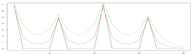
We now provide a very short empirical comparison of the LASSO and Generalized LASSO approach in a toy example of such a model. Note that for $\alpha\geq 0$, $\beta^{*}=X^{\alpha}g$ being a smoothed version of $g$, is “almost sparse”, so a comparison with the LASSO makes sense. We propose the following setting: let $M(\rho)=(\rho^{|i-j|})_{1\leq i,j\leq n}$, and $X=M^{1/2}$. We take $g=(7,0,0,0,0,5,0,0,0,0,7,0,0,0,0,5,0,0,0,0)$, $n=20$, $\rho=0.5$, Figure 1 gives the different values of $\beta^{*}=X^{\alpha}g$ for various values of $\alpha$.

Figure 1: The parameter $\beta^{*}=X^{\alpha}g$ for different values of $\alpha$. In black, $\alpha=0$, so $\beta^{*}=g$ is sparse. In red, $\alpha=1$, $\beta^{*}$ is a bit smoothed, but still can be approximated by a sparse signal. In green, $\alpha=2$, $\beta^{*}$ is smoother, and approximation by a sparse signal do not hold any longer.

We compute the LASSO and Generalized LASSO in each case, and report the performance of the oracle with respect to the regularization parameter $s$:

$${\rm Perf.GL}=\inf_{s>0}\|X\hat{\beta}^{GL}_{s}-X\beta^{*}\|\text{ and }{\rm Perf.L}=\inf_{s>0}\|X\hat{\beta}^{L}_{s}-X\beta^{*}\|.$$

Of course, in practice, the optimal $s$ in unknown and may be estimated by cross-validation for example. We test both estimators with several values for the parameters $\alpha$ and $\sigma^{2}$. For each value of these parameters, we run $20$ experiments and report the mean performances for both estimators. The results are given in Table 1. We can see that the results seem coherent with Theorem 1: there seems to be an advantage in practice to consider the Generalized LASSO in the cases where $alpha\neq 0$.

Table 1: The mean results for $20$ experiments for each value of $(\alpha,\sigma^{2})$.

$\alpha$	$\sigma^{2}$	mean of ${\rm Perf.L}$	mean of ${\rm Perf.GL}$
	0.01	0.167	0.118
-2	0.30	4.792	3.076
	1.00	16.636	10.328
	0.01	0.194	0.097
-1	0.30	5.624	2.911
	1.00	14.386	8.56
	0.01	0.098	0.098
0	0.30	2.835	2.835
	1.00	9.012	9.012
	0.01	0.196	0.094
+1	0.30	5.144	2.517
	1.00	13.232	8.597
	0.01	0.199	0.101
+2	0.30	5.589	3.018
	1.00	17.957	10.228
	0.01	0.183	0.102
+3	0.30	5.538	3.175
	1.00	19.133	10.371

4 Proofs

4.1 Proof of Lemma 1

We have $Y\sim\mathcal{N}(X\beta^{*},\sigma^{2}I_{n})$ and so $Y-X\beta^{*}\sim\mathcal{N}(0,\sigma^{2}I_{n})$ and finally $X^{\prime}(Y-X\beta^{*})\sim\mathcal{N}(0,\sigma^{2}X^{\prime}X)$. Let us put $V=X^{\prime}(Y-X\beta^{*})$ and let $V_{j}$ denote the $j$-th coordinate of $V$. Note that $X^{\prime}X$ is normalized such that for any $j$, $V_{j}\sim\mathcal{N}(0,\sigma^{2})$, so: $\mathds{P}\left(|V_{j}|>s\right)\leq\exp(-s^{2}/(2\sigma^{2}))$. Then $\mathds{P}\left(\|V\|_{\infty}>s\right)\leq p\exp(-s^{2}/(2\sigma^{2}))$. ∎

4.2 Proof of Theorem 1

We use arguments from [BRT09]. From now, we assume that the event $\{\beta^{*}\in\mathcal{DC}(s/2)\}=\{\|X^{\prime}(Y-X\beta^{*}\|_{\infty}<s/2\}$ is satisfied. According to Lemma 1, the probability of this event is at least $1-p\exp(-s^{2}/(8\sigma^{2}))=1-\varepsilon$ as $s=2(2\log(p/\varepsilon))^{1/2}$.

Proof of the results on the Generalized Dantzig Selector.

We have

$$(\hat{\beta}^{GDS}_{s}-\beta^{*})^{\prime}G(\hat{\beta}^{GDS}_{s}-\beta^{*})=(\hat{\beta}^{GDS}_{s}-\beta^{*})^{\prime}X^{\prime}XF(\hat{\beta}^{GDS}_{s}-\beta^{*})\\ \leq\|X^{\prime}X(\hat{\beta}^{GDS}_{s}-\beta^{*})\|_{\infty}\|F(\hat{\beta}^{GDS}_{s}-\beta^{*})\|_{1}\\ \leq\left(\|X^{\prime}(Y-X\beta^{*})\|_{\infty}+\|X^{\prime}(Y-X\hat{\beta}^{GDS}_{s})\|_{\infty}\right)\|F(\hat{\beta}^{GDS}_{s}-\beta^{*})\|_{1}\\ \leq(s/2+s)\|F(\hat{\beta}^{GDS}_{s}-\beta^{*})\|_{1}$$

since $\hat{\beta}^{GDS}_{s}\in\mathcal{DC}(s)$, and $\{\beta^{*}\in\mathcal{DC}(s/2)\}$ is satisfied. By definition of $\hat{\beta}^{GDS}_{s}$,

$$0\leq\|F\beta^{*}\|_{1}-\|F\hat{\beta}^{GDS}_{s}\|_{1}\\ =\sum_{(F\beta^{*})_{j}\neq 0}|(F\beta^{*})_{j}|-\sum_{(F\beta^{*})_{j}\neq 0}|(F\hat{\beta}^{GDS}_{s})_{j}|-\sum_{(F\beta^{*})_{j}=0}|(F\hat{\beta}^{GDS}_{s})_{j}|\\ \leq\sum_{(F\beta^{*})_{j}\neq 0}|(F\beta^{*})_{j}-(F\hat{\beta}^{GDS}_{s})_{j}|-\sum_{(F\beta^{*})_{j}=0}|(F\beta^{*})_{j}-(F\hat{\beta}^{GDS}_{s})_{j}|.$$

This means that

$$\|F(\hat{\beta}^{GDS}_{s}-\beta^{*})\|_{1}\leq 2\sum_{(F\beta^{*})_{j}\neq 0}|(F\beta^{*})_{j}-(F\hat{\beta}^{GDS}_{s})_{j}|.$$

We can summarize all that we have now:

$$(\hat{\beta}^{GDS}_{s}-\beta^{*})^{\prime}G(\hat{\beta}^{GDS}_{s}-\beta^{*})\leq\frac{3s}{2}\|F(\hat{\beta}^{GDS}_{s}-\beta^{*})\|_{1}\\ \leq 3s\sum_{(F\beta^{*})_{j}\neq 0}|(F\beta^{*})_{j}-(F\hat{\beta}^{GDS}_{s})_{j}|.$$ (2)

Let us remark that Inequality (2) implies that the vector $\alpha=F(\hat{\beta}^{GDS}_{s}-\beta^{*})$ may be used in Assumption $A(c)$. This leads to

$$(\hat{\beta}^{GDS}_{s}-\beta^{*})^{\prime}G(\hat{\beta}^{GDS}_{s}-\beta^{*})\leq 3s\sum_{(F\beta^{*})_{j}\neq 0}|(F\beta^{*})_{j}-(F\hat{\beta}^{GDS}_{s})_{j}|\\ \leq 3s\sqrt{\|F\beta^{*}\|_{0}\sum_{(F\beta^{*})_{j}\neq 0}[(F\beta^{*})_{j}-(F\hat{\beta}^{GDS}_{s})_{j}]^{2}}\\ \leq 3s\sqrt{\|F\beta^{*}\|_{0}c(F\hat{\beta}^{GDS}_{s}-F\beta^{*})^{\prime}H(F\hat{\beta}^{GDS}_{s}-F\beta^{*})}\\ =3s\sqrt{\|F\beta^{*}\|_{0}c(\hat{\beta}^{GDS}_{s}-\beta^{*})^{\prime}G(\hat{\beta}^{GDS}_{s}-\beta^{*})}.$$ (3)

As a consequence,

$$(\hat{\beta}^{GDS}_{s}-\beta^{*})^{\prime}A(\hat{\beta}^{GDS}_{s}-\beta^{*})\leq 9s^{2}\|P\beta^{*}\|_{0}c=72\sigma^{2}c\|P\beta^{*}\|_{0}\log(p/\varepsilon).$$

Plugging this result into Inequality (3) and using Inequality (2) again, we obtain:

$$\|P(\hat{\beta}^{GDS}_{s}-\beta^{*})\|_{1}\leq 18\sqrt{2}\sigma\|P\beta^{*}\|_{0}\sqrt{c\log(p/\varepsilon)}.$$

Proof of the results on the Generalized LASSO.
Step 1. As a fist step, we establish an important property of the Generalized LASSO estimator. We prove that

$$\forall\beta\in\mathds{R}^{p},\quad|Y-XF\hat{\beta}^{GL}_{s}\|_{2}^{2}+2s\|F\hat{\beta}^{GL}_{s}\|_{1}+(\hat{\beta}^{GL}_{s})^{\prime}F(H-X^{\prime}X)F\hat{\beta}^{GL}_{s}\\ \leq\|Y-XF\beta\|_{2}^{2}+2s\|F\beta\|_{1}+\beta^{\prime}F(H-X^{\prime}X)F\beta.$$ (4)

To prove Inequality (4), we write the Lagrangian of the program that defines $\hat{\beta}^{GL}_{s}$:

$$\mathcal{L}(\beta,\lambda,\mu)=\beta^{\prime}G\beta+\lambda^{\prime}\left[X^{\prime}(X\beta-Y)-sE\right]+\mu^{\prime}\left[X^{\prime}(Y-X\beta)-sE\right],$$

where $E=(1,\ldots,1)^{\prime}$, $\lambda$ and $\mu$ are vectors in $\mathds{R}^{p}$. Any solution $\underline{\beta}=\underline{\beta}(\lambda,\mu)$ must satisfy, for some $\lambda_{j}\geq 0$, $\mu_{j}\geq 0$ and $\lambda_{j}\mu_{j}=0$,

$$0=\frac{\partial\mathcal{L}}{\partial\beta}(\underline{\beta},\lambda,\mu)=2G\beta+X^{\prime}X(\lambda-\mu),$$

and then $G\underline{\beta}=(X^{\prime}X)(\mu-\lambda)/2$ . Note that $\lambda_{j}\geq 0$, $\mu_{j}\geq 0$ and $\lambda_{j}\mu_{j}=0$ imply that there is a $\gamma_{j}\in\mathds{R}$ such that $\gamma_{j}=(\mu_{j}-\lambda_{j})/2$, $|\gamma_{j}|=(\lambda_{j}+\mu_{j})/2$. Hence $\lambda_{j}=2(\gamma_{j})_{-}$ and $\mu_{j}=2(\gamma_{j})_{+}$, where for any $a$, $(a)_{+}=max(a;0)$ and $(a)_{-}=max(-a;0)$. Let also $\gamma$ denote the vector which $j$-th component is exactly $\gamma_{j}$, we obtain:

$$G\underline{\beta}=(X^{\prime}X)\gamma.$$ (5)

Then we have easily $\underline{\beta}^{\prime}F\underline{\beta}=\underline{\beta}^{\prime}(X^{\prime}X)\gamma=\gamma^{\prime}H\gamma$. Using these relations, the Lagrangian may be written:

$$\mathcal{L}(\underline{\beta},\lambda,\mu) = \gamma^{\prime}H\gamma+2\gamma^{\prime}X^{\prime}Y-2\gamma^{\prime}(X^{\prime}X)\underline{\beta}-2s\sum_{j=1}^{p}|\gamma_{j}|$$

$$= 2\gamma^{\prime}X^{\prime}Y-\gamma^{\prime}H\gamma-2s\left\|\gamma\right\|_{1}$$

Note that $\lambda$ and $\beta$, and so $\gamma$, should maximize this value. Hence, $\gamma$ is to minimize

$$-2\gamma^{\prime}X^{\prime}Y+\gamma^{\prime}H\gamma+2s\|\gamma\|_{1}+Y^{\prime}Y$$

Now, note that

$$Y^{\prime}Y-2\gamma^{\prime}X^{\prime}Y=\|Y-X\gamma\|_{2}^{2}-\gamma^{\prime}(X^{\prime}X)\gamma$$

and then $\gamma$ also minimizes

$$\|Y-X\gamma\|_{2}^{2}+2s\left\|\gamma\right\|_{1}+\gamma^{\prime}\left[H-(X^{\prime}X)\right]\gamma.$$

We end the proof of (4) by noting that for every $b$ such that $Fb=\gamma$, then $b$ is to minimize

$$\|Y-XFb\|_{2}^{2}+2s\left\|Fb\right\|_{1}+(Fb)^{\prime}\left[H-(X^{\prime}X)\right](Fb).$$ (6)

and that $\hat{\beta}^{GL}_{s}$ is such a $b$.

Step 2. The next step is to apply Equation (4) with $\beta=\beta^{*}$ to obtain

$$\|Y-XF\hat{\beta}^{GL}_{s}\|_{2}^{2}+2s\|F\hat{\beta}^{GL}_{s}\|_{1}+(\hat{\beta}^{GL}_{s})^{\prime}F(H-X^{\prime}X)F\hat{\beta}^{GL}_{s}\\ \leq\|Y-XF\beta^{*}\|_{2}^{2}+2s\|F\beta^{*}\|_{1}+(F\beta^{*})^{\prime}(H-X^{\prime}X)F\beta^{*}.$$

For the sake of simplicity, we can define $\hat{\gamma}=F\hat{\beta}^{GL}_{s}$ (following the notations of Step 1) and $\gamma^{*}=F\beta^{*}$ and we obtain

$$\|Y-X\hat{\gamma}\|_{2}^{2}+2s\|\hat{\gamma}\|_{1}+\hat{\gamma}^{\prime}(H-X^{\prime}X)\gamma\\ \leq\|Y-X\gamma^{*}\|_{2}^{2}+2s\|\gamma^{*}\|_{1}+(\gamma^{*})^{\prime}(H-X^{\prime}X)\gamma^{*}.$$

Computations lead to

$$\|X(\hat{\gamma}-\gamma^{*})\|_{2}^{2}+2s\|\hat{\gamma}\|_{1}+\hat{\gamma}^{\prime}(H-X^{\prime}X)\hat{\gamma}-2(Y-X\gamma^{*})^{\prime}X\hat{\gamma}\\ +2(\gamma^{*})^{\prime}(H-X^{\prime}X)(\gamma^{*}-\gamma)\leq 2s\|\gamma^{*}\|_{1}+(\gamma^{*})^{\prime}(H-X^{\prime}X)\hat{\gamma}-2(Y-X\gamma^{*})^{\prime}X\gamma^{*},$$

and then

$$\|X(\hat{\gamma}-\gamma^{*})\|_{2}^{2}\\ \leq 2s(\|\gamma^{*}\|_{1}-\|\hat{\gamma}\|_{1})+2(Y-X\gamma^{*})^{\prime}X(\hat{\gamma}-\gamma^{*})-(\gamma^{*}-\hat{\gamma})^{\prime}(H-X^{\prime}X)(\gamma^{*}-\hat{\gamma}).$$

As a consequence

$$(\gamma^{*}-\hat{\gamma})^{\prime}H(\gamma^{*}-\hat{\gamma})\leq 2s(\|\gamma^{*}\|_{1}-\|\hat{\gamma}\|_{1})+2(Y-X\gamma^{*})^{\prime}X(\hat{\gamma}-\gamma^{*})\\ \leq 2s\sum_{j=1}^{p}(|\gamma_{j}^{*}|-|\hat{\gamma}_{j}|)+2\|X^{\prime}(Y-X\beta^{*})\|_{\infty}\sum_{j=1}^{p}|\hat{\gamma}_{j}-\gamma^{*}_{j}|\\ \leq 2s\sum_{j=1}^{p}(|\gamma_{j}^{*}|-|\hat{\gamma}_{j}|)+s\sum_{j=1}^{p}|\hat{\gamma}_{j}-\gamma^{*}_{j}|.$$

So we obtain

$$(\gamma^{*}-\hat{\gamma})^{\prime}H(\gamma^{*}-\hat{\gamma})+s\sum_{j=1}^{p}|\hat{\gamma}_{j}-\gamma^{*}_{j}|\leq 2s\sum_{j=1}^{p}(|\hat{\gamma}_{j}|-|\gamma^{*}_{j}|)+2s\sum_{j=1}^{p}|\hat{\gamma}_{j}-\gamma^{*}_{j}|\\ =2s\sum_{j:\gamma^{*}_{j}\neq 0}(|\hat{\gamma}_{j}|-|\gamma^{*}_{j}|)+2s\sum_{j:\gamma^{*}_{j}\neq 0}|\hat{\gamma}_{j}-\gamma^{*}_{j}|=4s\sum_{j:\gamma^{*}_{j}\neq 0}|\hat{\gamma}_{j}-\gamma^{*}_{j}|.$$ (7)

In particular, Equation (7) implies that

$$\sum_{j:\gamma^{*}_{j}=0}|\hat{\gamma}_{j}-\gamma^{*}_{j}|\leq 3\sum_{j:\gamma^{*}_{j}\neq 0}|\hat{\gamma}_{j}-\gamma^{*}_{j}|,$$

and so $\alpha=\hat{\gamma}_{j}-\gamma^{*}_{j}$ may be used in Assumption $A(c)$. Then Inequality (7) becomes

$$(\gamma^{*}-\hat{\gamma})^{\prime}H(\gamma^{*}-\hat{\gamma})\leq 4s\sum_{j:\gamma^{*}_{j}\neq 0}|\hat{\gamma}_{j}-\gamma^{*}_{j}|\leq 4s\sqrt{\|\gamma^{*}\|_{0}\sum_{j:\gamma^{*}_{j}\neq 0}(\hat{\gamma}_{j}-\gamma^{*}_{j})^{2}}\\ \leq 4s\sqrt{\|\gamma^{*}\|_{0}c(\gamma^{*}-\hat{\gamma})^{\prime}H(\gamma^{*}-\hat{\gamma})}.$$

That leads to

$$(\hat{\beta}^{GL}_{s}-\beta^{*})^{\prime}G(\hat{\beta}^{GL}_{s}-\beta^{*})=(\gamma^{*}-\hat{\gamma})^{\prime}H(\gamma^{*}-\hat{\gamma})\leq 128\sigma^{2}c\|F\beta^{*}\|_{0}\log(p/\varepsilon).$$ (8)

We plug (8) into (7) again to obtain $\|\hat{\gamma}-\gamma^{*}\|_{1}\leq 32\sqrt{2}\sigma\|P\beta^{*}\|_{0}\sqrt{c\log(p/\varepsilon)}$. ∎