Structural Transitions in A Crystalline Bilayer : The Case of Lennard Jones and Gaussian Core Models

Abstract

We study structural transitions in a system of interacting particles arranged as a crystalline bilayer, as a function of the density $\rho$ and the distance $d$ between the layers. As $d$ is decreased a sequence of transitions involving triangular, rhombic, square and centered rectangular lattices is observed. The sequence of phases and the order of transitions depends on the nature of interactions.

1 Introduction

Structural transitions in solids may be caused by various external parameters such as temperature, pressure, stress, electrical and magnetic fields [1, 2]etc. Confinement and dimensional reduction can also lead to structural transitions especially in soft solids like colloidal suspensions. Colloidal solids are especially suited to modification and manipulation using a variety of means such as structural confinement [3], laser-induced phase transitions [4], shear [5], static [6] and dynamic [7] external fields.

Confined colloids kept in a thin wedge geometry of two optically-flat quartz glass plates, exhibit a sequence of structural transitions : $n\triangle\rightarrow(n+1)\Box\rightarrow(n+1)\triangle$ with increasing wedge height, where $n$ is the number of layers and $\triangle$ and $\Box$ corresponds to layers of triangular($p6$) and square($p4m$) symmetry respectively [8, 9]. The full equilibrium phase diagram of such a system has been studied analytically as well as using extensive computer simulations[10, 11]. The transitions are usually first order, though continuous transitions via a layer buckling mechanism [12] has also been predicted and observed.

In this paper, we explore another way in which structural transitions may be induced in a colloidal solid. Consider a crystalline bilayer separated by a distance $d$ between the layers. Each of these layers is held in place by individual trapping potentials, set up, for example using laser tweezers [13]. The strong trapping potential ensures that out of layer fluctuations are typically unimportant. We investigate the stability of the bilayer as the distance $d$ is decreased. We show that $d$ behaves as a controlling parameter and induces a rich sequence of transitions involving a variety of two-dimensional Bravais lattices. The exact sequence of transitions crucially depends on the nature of interactions. In this paper we study two kinds of model solids (a) the generic Lennard Jones (LJ) [14] solid and (b) the soft Gaussian core model (GCM) [15] appropriate for suspensions of globular polymers. Our main results are as follows. For the LJ system, we obtain at temperature $T=0$ two independent triangular (TRN) crystalline layers for large $d$. As $d$ is reduced, the system undergoes a first order transition to a staggered square (SQR) solid. As $d$ is further reduced, this square solid becomes, first, a centered rectangular (CR) and finally again a triangular solid as $d$ is decreases to zero and the layers merge. The final two transitions are continuous.

In contrast for the GCM, all the transitions are continuous. As $d$ reduces, the TRN solid transforms to a SQR solid continuously through a sequences of rhombic (RMB) lattices. The SQR solid subsequently transforms back to the TRN solid for small values of $d$ again continuously but this time it uses a sequence of CR lattices with intermediate aspect ratios. The progression of phases seen correspond roughly with those seen in the extensive literature on classical interacting bilayer Wigner crystals [16], though the sequence of phases and the nature of transitions are different.

The rest of the paper is organized as below. In the next section, we describe the bilayer system in detail, introducing the order parameters for the transition and state the interatomic potentials used. In Section 3,we give the results for the zero temperature energy minimization. This is followed in Section 4 by a full normal mode analysis investigating the stability of the ground states obtained in Section 3 and the nature of the transition. In Section 5, we present results of finite temperature Monte Carlo simulations. We discuss our results and their implications and conclude in Section 6.

2 Model System

Figure 1: A schematic diagram of the model bilayer solid explaining the structural parameters. The crystal structure on each of the layers, denoted by filled and open circles, are identical but staggered by the amount $\lambda$ along the diagonal. The lattice parameetrs are $a$ and $b$ and the apex angle is $\phi$. The half filled circle is the projection of a lattice point (filled circle) on the top layer to the bottom one.

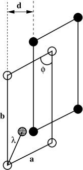
Consider a system of $2N$ particles arranged as two parallel two-dimesional crystalline layers of $N$ particles each (see Fig.(1)). The crystal structure of each of these layers may be assumed to be a general two-dimensional oblique ($p2$) lattice. Each particle interacts with all other particles via isotropic and pair-wise interacting potentials. The position vector for the $i$-th particle of this lattice can thus be expressed as

$$\vec{r}_{i} = (m+\lambda)\vec{a}+(n+\lambda)\vec{b}+d\hat{z}$$ (1)

$$= ((m+\lambda)a+(n+\lambda)b{}\cos\phi){}\hat{x}+{}(n+\lambda){}b{}\sin\phi{}\hat{y}+d{}\hat{z}$$

where $m,n=0,1,2,\cdots$, $\vec{a}$ and $\vec{b}$ are two in-plane basis vectors, $\phi$ is the angle between these two basis vectors,$d$ is the interlayer separation and $\lambda$ is a shift between the center of masses of two layers (Fig.(1)). Therefore to specify our model completely, knowledge of these five variables, $a,b,\phi,d,\lambda$ is sufficient. The last variable $\lambda$ ensures that for small values of $d$, the particles from different layers do not overlap. The particles are not allowed to fluctuate out of the layers and particle exchange between the layers is prohibited. Each layer is therefore considered to be strongly confined in the Z-direction while they are allowed complete freedom in the X,Y- plane.

Let us first imagine the possible physical scenario as the layers are brought close to each other starting from a large inter-layer separation. When the layers are well apart they exist as two independent mono-layers and they show TRN symmetry, the minimum energy configuration for the two-dimensional crystalline system for the interaction potentials considered by us. As the inter-layer separation, $d$, between these two layers starts decreasing, the system passes through a series of structural transitions which may involve RMB and SQR phases. For even smaller values of $d$, two layers start merging into one and the TRN symmetry is regained. Transformation between a SRQ and a TRN phase may be accomplished, in general, by either (i) shear i.e. change in the angle between two in-plane basis vectors producing an intermediate RMB structure or (ii) change in the aspect ratio ($b/a$) which produces a CR lattice. Both the RMB and the CR lattices being less symmetric have TRN and SQR phases as limiting cases.

It is therefore clear that we need to introduce two order parameters [17] in order to describe completely the phase transitions of our model system. First, the bond angle order parameter $\psi=\cos\phi$ which is $0$ when system takes SQR symmetry ($\phi=90^{\circ}$) and non-zero otherwise. The second order parameter $\xi$ is related to the aspect ratio $b/a$ as $\xi=(b/a-1)/(\sqrt{3}-1)$ which varies from $0$ in the SQR to a non-zero value in the CR phase. Note that the highly symmetric TRN phase is described both by ($\psi=0.5,\xi=0$) and ($\psi=0.0,\xi=1$). Finally, if $\epsilon_{ij},i,j=x,y$ is the two dimensional strain tensor, the shear, $e_{3}=\epsilon_{xy}$, and deviatoric, $e_{2}=\epsilon_{xx}-\epsilon_{yy}$, strains are related to $\theta$ and $\xi$ as,

$$\tan{}\phi = \epsilon_{3}/(1-\epsilon_{1})$$

$$\phantom{xxx}{}\xi = \frac{2(1+\epsilon_{2})+\epsilon_{1}}{2(1-\epsilon_{2})+\epsilon_{1}}$$ (2)

We have studied phase transitions in the bilayer system for two different model potentials. The Lennard Jones potential :

$$U = \sum_{i\neq j}V_{LJ}(r_{ij})$$ (3)

$$= 4\epsilon\biggl{[}\biggl{(}\frac{\sigma}{r_{ij}}\biggr{)}^{12}-\biggl{(}\frac{\sigma}{r_{ij}}\biggr{)}^{6}\biggr{]}$$

has been used extensively in the past as a generic model which includes both long range attractive and short range repulsive interactions. In Eq. (3), $r_{ij}=|\vec{r}_{i}-\vec{r}_{j}|$, the distance between the $i$ and $j$-th particle. An intrinsic length scale $r_{min}=2^{1/6}\sigma$ corresponding to the minimum of $V_{LJ}$ may be associated with this potential. The nearest neighbour distance between particles is close to this value throughout. We use reduced units for LJ potential throughout the paper defining lengths in units of $\sigma$ and energy in units of $\epsilon$. It follows that the densities are in units of $\sigma^{-3}$ and temperatures in units of $\epsilon/k_{B}$, where $k_{B}$ is the Boltzmann factor.

On the other hand, Gaussian core potential has been used specifically to model soft solids.

$$U = \sum_{i\neq j}V_{GCM}(r_{ij})$$ (4)

$$= \sum_{i\neq j}V_{0}exp[-(r_{ij}/l)^{2}],\phantom{xxx}V_{0},l>0$$

$V_{0}$ and $l$ acts as the energy and length-scales for this potential and $r_{ij}$ is same as it was for the previous equation. The GCM is interesting because, firstly, the potential is soft and is known to display behaviour similar to that of real polymeric solids. Also many of its properties are well known and tested especially because at very low densities it reduces to the hard disk model which is widely used for modelling colloidal solids. Due to the purely repulsive nature of this potential, it does not have any preferred nearest neighbour distance which is determined in this case by the density. This potential also possesses an interesting duality property [18] such that high ($\rho_{>}$) and low ($\rho_{<}$) density properties are related to each other by

$$\rho_{>}\rho_{<}=\pi^{-D}$$ (5)

where $D$ is the dimensionality. It is therefore sufficient to confine our studies in the range $0<\rho<\rho_{f.p.}$ where the fixed point density $\rho_{f.p.}=\pi^{-1}\simeq 0.32$ in two-dimensions.

3 Zero Temperature Calculation

In this section, we determine the ground states of our system in the space of the order parameters, $\phi$ and $\xi$, keeping the layer separation $d$ and the density $\rho$ as external parameters. Below we discuss our results for the LJ solid and the GCM one after the other.

3.1 Lennard-Jones potential

We begin with $2N$ particles divided into two layers each arranged in a TRN lattice of $N$ particles. For fixed layer separation $d$, and the lattice parameter $a$ set by the density $\rho$, we minimize the total energy $U$ with respect to $\lambda$ and $b$. The resulting order parameter $\xi$ remains constant at $1$ – the value appropriate for the TRN lattice. For the lattice sums needed to calculate the minimized energy we have set a cut-off radius, $r_{c}=2.5\sigma$.

Figure 2: (a) Plots of the total energy as a function of $\psi$ at $\rho=1.2$ and (top to bottom) $d=0.66,0.68,0.70$and $0.72$ showing the SQR to TRN transition for the LJ system. (inset) The energies of the SQR (filled square) and TRN (filled triangles) plotted as a function of $d$ are seen to cross with a change in slope as expected of a first order transition. The fact that this transition is first order has also been verified by a normal mode analysis. (b) Plot of the order parameter $\xi$ as a function of $d$ at the same density showing the two continuous transitions SQR $\to$ CR $\to$ TRN as $d\to 0$.

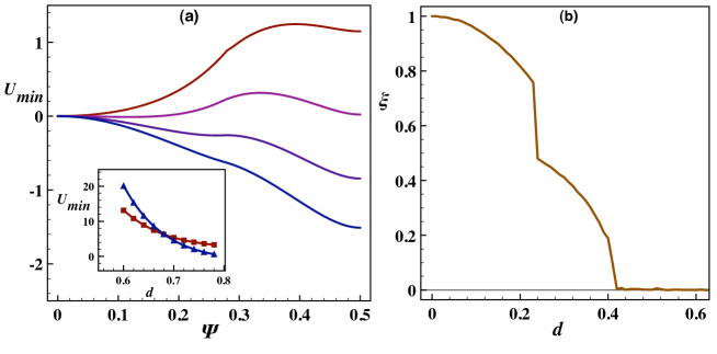
In Fig.(2a) we have plotted minimized energy $U_{min}$ as a function of the order parameter $\psi$ for various values of $d$. For large inter-layer separation, bond angle order parameter at the minimized energy ($U_{min}$) shows a non-zero value, $\psi=\cos\phi=0.5$, which indicates TRN symmetry ($\phi=60^{\circ}$). The minimum in $\lambda$ is very shallow indicating two triangular lattices prefer to remain independent. As $d$ is decreased two layers fall into registry and for further decrease of $d$ a second minimum at $\psi=0$ develops corresponding to the SQR phase ($\phi=90^{\circ}$). A plot of the energy of the SQR and TRN phase (Fig.(2a) inset) shows a first order transition at $d=0.684$. This fact is confirmed by a normal-mode analysis presented in the next section.

At even smaller values of $d$, the square solid begins to deform continuously by changing the aspect ratio (or order parameter $\xi$) at fixed $\phi$. In Fig.(2b) we have plotted the minimized value of $\xi$ vs. $d$. From the plot it is obvious that there are two distinct continuous transitions taking the solid from SQR at $\xi=0$ to an eventual TRN phase at $\xi=1$ via an intermediate CR lattice of $\xi=0.5$.

3.2 Gaussian Core Model

Figure 3: (a) Plot of the total energy in the GCM for $\rho=0.2$ and (top to bottom) $d=1.4,1.5,1.6,1.7$ and $1.9$ as a function of $\psi$. Note the appearance of the minimum at $\psi=0.5$ corresponding to the TRN lattice as $d$ increases. (b) The continuous transition from the SQR to the TRN lattice as $d\to 0$.

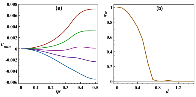
Due to the purely repulsive nature of the Gaussian core potential, it does not have any preferred nearest neighbour distance and at zero stress the solid would disintegrate. We have carried out all minimizations for a system with fixed reduced density, $\rho=0.2$. We have plotted the minimized energy $U_{min}$ as a function of the bond angle order parameter $\phi$ for various values of $d$. In Fig.(3a) in contrast to the Lennard-Jones solid we now obtain continuous transitions from TRN to SQR through a set of RMB phases and back to TRN at $d=0$ through a set of CR phases.

3.3 T=0 Phase Diagram

Figure 4: Zero temperature phase diagrams in the $\rho-d$ plane for the LJ (a) and GCM (b) systems. The various phases are marked. First order transitions are shown by solid and continuous transitions by dashed lines.

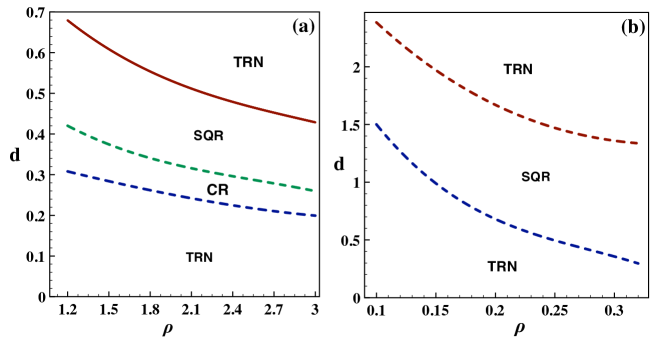
Our results concerning the various ground states and structural transitions in both the LJ and GCM systems in the $\rho$ - $d$ plane has been shown in the zero temperature phase diagrams, Fig.(4a) and (b) respectively. Note that for both the systems the triangular phase is stable at all $\rho$ for both very large $d$ and $d=0$ where the system becomes effectively two dimensional.

4 Normal Mode Analysis

To further elucidate the nature of the structural transitions in the two systems, we have undertaken a normal mode analysis [19] of the TRN and SQR solids obtained for each of the two interactions.

Let $\vec{u}(\vec{r}_{i})$ be the displacement of the $i$-th particle from its equilibrium position $\vec{r}_{i}$. Within harmmonic approximation, now the potential can be written as

$$U_{harm}=\frac{1}{2}\sum_{i,j}\vec{u}(\vec{r}_{i})\mathcal{D}(\vec{r}_{i}-\vec{r}_{j})\vec{u}(\vec{r}_{j})$$ (6)

$$\mathcal{D}(\vec{r}_{i}-\vec{r}_{j}) = D_{\mu\nu}(\vec{r}_{i}-\vec{r}_{j})$$ (7)

$$= \delta_{\vec{r}_{i}\vec{r}_{j}}\sum_{k}V_{\mu\nu}(\vec{r}_{i}-\vec{r}_{k})-V_{\mu\nu}(\vec{r}_{i}-\vec{r}_{j})$$

where $V_{\mu\nu}(\vec{r})=\partial^{2}V/\partial r_{\mu}\partial r_{\nu}$. We have $2N$ equations of motion, one for each of the three components of the $N$ particles, since we have already restricted fluctuation in the $z$-direction.

$$\ddot{\vec{u}}(\vec{r}_{i})=-\sum_{j}\mathcal{D}(\vec{r}_{i}-\vec{r}_{j})\vec{u}(\vec{r}_{j})$$ (8)

We seek solutions to the equations of motion in the form of simple plane waves :

$$\vec{u}(\vec{r},t)=\vec{\epsilon}\phantom{x}exp[i(\vec{k}.\vec{r}-\omega t)]$$ (9)

Here $\vec{\epsilon}$ is the polarization vector of the normal mode. The Born-vonKarman periodic boundary conditions restricts the wave vector $\vec{k}$ to a single primitive cell of the reciprocal lattice vector, which is normally identified with the first Brillouin zone.

Figure 5: Results for phonon dispersion curves : (a) diagram showing the high symmetry points in the SQR and TRN (reciprocal) lattices. (b) Phonon dispersion for the stable SQR lattice at $\rho=1.2$ and $d=d_{c}=0.684$ i.e. the value of $d$ at SQR to TRN transition. Note that the dispersion curve shows that the SQR phase is locally stable pointing to a first order transition. (c) Phonon dispersion of the SQR solid at $\rho=1.2$ and $d=0.4$ showing an instability in the transverse acoustic branch. At this value of $d$ the CR solid is stable. (d) Dispersion curve for the TRN solid in the GCM for $\rho=0.2$ and $d=1.6$ showing the appearance of a non zero $k$ vector soft mode.

Substituting Eq.(8) into Eq.(7) we find a solution of the three-dimensional eigen value problem :

$$\omega^{2}\vec{\epsilon}=\mathcal{D}(\vec{k})\vec{\epsilon}$$ (10)

Here $\mathcal{D}(\vec{k})$, the dynamical matrix, is given by

$$\mathcal{D}(\vec{k})=\sum_{i}\mathcal{D}(\vec{r}_{i})e^{-i\vec{k}.\vec{r}_{i}}$$ (11)

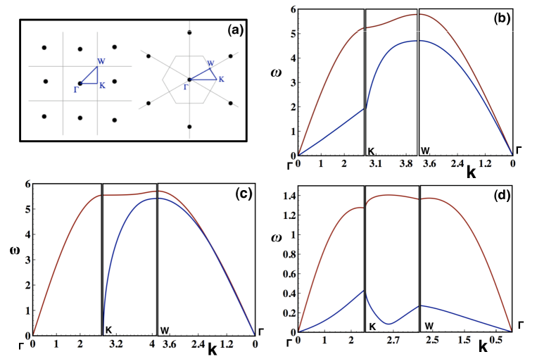
Two solutions to Eq.(9) for each of the $N$ allowed values of $\vec{k}$ give us $2N$ normal modes. The reciprocal lattices for both SQR and TRN are known to have the same symmetry of the real space lattice. Exploiting this property, one finds the values of $\omega$ only for those $k$-values along the lines connecting the high symmetry points of the first Brillouin zone (Fig.(5a)) thereby obtaining the dispersion curve $\omega$ vs $|\vec{k}|$ and mode structure of a given lattice. For any stable equilibrium structure $\omega$ should always be non-negative definite.

4.1 The Lennard Jones potential

To show that the SQR $\rightleftharpoons$ TRN transition at large $d$ is indeed first order, we have obtained the dispersion curves for the metastable SQR phase for a value of $d$ slightly larger than the critical $d_{c}=0.684$ for the chosen $\rho=1.2$. This is shown in Fig.(5b). This indicates that the transition is first order with the possibility of co-existence. When $d$ is decreased further, $\psi$ at the minimized energy $U_{min}$ shows minima at $\psi=0$ but the normal mode analysis shows us that the SQR structure can not be stable at this value of $d$ (Fig.(5c)). Actually, the two layers start merging into one, by changing the aspect ratio away from $b/a=1$.

4.2 The Gaussian Core Model

For the Gaussian core model the scenario is quite different. For intermediate values of $d$, the SQR structure is seen to be unstable and the mode structure for the TRN structure exhibits mode softening, Fig.(5d)), such that $\omega\to 0$ for $k\neq 0$. Examination of the deformation corresponding to this $\vec{k}$ shows that the SQR lattice becomes unstable to shear deformation at the zone boundary. This mode softening therefore establishes the transition from TRN to SQR transition to be continuous for the Gaussian core model.

The transition from SQR back to TRN at low $d$ is always continuous both for LJ and GCM as verified by our normal mode analysis.

5 Finite Temperature results:

We close our discussion on structural transitions in a bilayer crystal by briefly mentioning some of our results for the LJ case using Monte Carlo simulations [20]. A detailed calculation of the phase diagram of the bilayer GCM in the temperature, $\rho$ and $d$ space using both Monte Carlo and classical mean field density functional theory, which is known to yeild particularly good results for this system, will be published elsewhere.

Figure 6: Configurations from our Monte Carlo simulation in the LJ system for $T=1.0$. (a) and (b) show the result of increasing $d$ from $d=0.6$ to $d=0.8$ at fixed $\rho=1.20$. Note the first order SQR to TRN transition. (c) and (d) show the corresponding result for pressure induced SQR to TRN transition as $\rho$ is increased from $1.3$ to $1.4$ at fixed $d=0.6$. Our results are consistent with those seen in Fig.(4a).

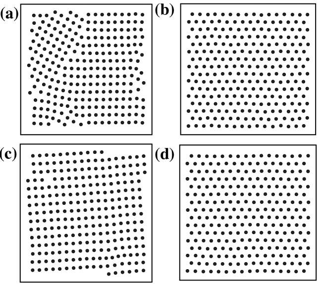
The simulation is done using the usual Metropolis algorithm keeping total number$(N)$ of particles, volume$(V)$ and temperature$(T)$ fixed. Periodic boundary conditions have been used for all directions except in the direction of stacking of the layers. For our purpose, we use a system of $512$ number of particles, temperature is fixed at $1.0$ and the volume is determined by the density, $\rho=1.2$, used for simulation. Starting from a large layer seperation $(d\gg 0)$, we have observed the system change its symmetry from TRN to SQR with decreasing $d$. For large values of $d$ ($d>0.8$), when the two layers are well seperated, each layer behaves independently of each other exhibiting the expected TRN structure. As $d$ is decreased, the two layers start interacting with each other. As a result, part of the system starts to transform into a SQR. Through this phase co-existence, the whole system transforms to a state where each layer shows SQR structure at $d=0.6$.

We have also explored the configurations of our model system in the temperature-density plane keeping the inter-layer separation fixed. For $d=0.6$, where we have already seen the SQR structure to be the ground state, we increase $\rho$ to $1.3$. We again encounter a first order boundary and the system equilibrates to the SQR structure.

The values of the critical $d$ and $\rho$ compare favourably with the $T=0$ phase diagram shown in Fig. (4a). Similar scans at other temperature values over a large range of $\rho$ and $d$ have confirmed that it is not possible to induce a structural transition in this model by changing $T$. The phase boundaries shown in Fig.(4) therefore extend vertically upto a melting temperature $T_{m}(\rho,d)$. This behavior is identical to that seen in the classical Wigner crystal and is probably an universal feature of any such crystalline bilayer.

6 Summary and Conclusion

In this paper we have studied structural transitions in a bilayer crystal. We have shown that the system has a rich phase diagram and shows a number of phase transitons. The identity of the phases and the nature of the transitions depend on the interaction potential. On the other hand, some features of these transitions e.g. the overall topology of the phase diagram seems to be similar and independent of the details of the interaction.

We believe that it may be easy to realize this soft matter system experimentally and study many of its interesting equilibrium and dynamic characteristics. For example, critical properties of the continuous structural transitions, especially, near the melting line and a detailed study of finite size scaling and crossover in these systems may be illuminating [21]. We are also particularly interested in the dynamics of the structural transitions for both the first order and continuous cases. Quenches from the SQR to the TRN lattice in this system may be accomplished simply by changing $d$. How does the new phase form inside the parent? Is there a possibility of a martensitic transition[22, 23]? If so, then of what type? We hope our work stimulates experiments designed to answer these questions in the near future.

7 Acknowledgement

We acknowledge useful discussions with K. G. Ayappa, M. Rao and A. Paul.

8 References

References

- [1] Chen et. al. 1992 Phys. Rev. Lett. 69 688
- [2] Wen et. al. 1999 Phys. Rev. Lett. 82 4248
- [3] Schmidt M and Löwen H 1996 Phys. Rev. Lett. 76 4552
- [4] Chaudhuri D and Sengupta S 2006 Phys. Rev. E 73 011507
- [5] Steveno M J, Robbins M O and Belak J F 1991 Phys. Rev. Lett. 66 3304
- [6] Chaudhuri A, Sengupta S and Rao M 2005 Phys. Rev. Lett. 95 266103
- [7] Sengupta A, Sengupta S and Menon G I 2007 it Phys. Rev. B 75 180201(R)
- [8] Pirenski P, Strzelecki L and Pansu B 1983 Phys. Rev. Lett. 50 900
- [9] Neser S, Bechinger C, Leiderer P and Palberg T 1997 Phys. Rev. Lett. 79 2348
- [10] Fortini A and Dijkstra M 2006 J. Phys. Cond. Matt. 18 L371
- [11] Ghatak C and Ayappa K G 2002 Journal of Chemical Physics 117 5373
- [12] Chou T and Nelson D R 1993 phys. Rev. E 48 4611
- [13] Metcalf H J and Straten P van der 1999 Laser Cooling and Trapping (Springer, Heidelberg)
- [14] Phillips J M, Bruch L W and Murphy R D 1981 J. Chem Phys. 75 5097
- [15] Stillinger F H and Weber T A 1981 J. Chem Phys. 74 4015
- [16] Goldoni G and Peeters F M 1996 Phys. Rev. B 53 4591
- [17] Hatch D M, Lookman T, Saxena A and Stokes H T 2001 Phys. Rev. B 64 060104(R)
- [18] Stillinger F H 1979 Phys Rev. B 20 299
- [19] Ashcroft N W and Mermin N D 1976 Solid State Physics (Saunders College, Philadelphia)
- [20] Frenkel D and Smit B 2002 Understanding Molecular Simulation: From Algorithm to Applications (Academic Press)
- [21] Chaikin P M and Lubensky T C 1995 Principles of Condensed Matter Physics ( Cambridge University Press, Cambridge)
- [22] Bhattacharya J, Paul A, Sengupta S, Rao M 2008 J. Phys. Condens. Matt. 20, 365210
- [23] Paul A, Bhattacharya J, Sengupta S, Rao M 2008 J. Phys. Condens. Matt. 20, 365211