Can disk-magnetosphere interaction models and beat frequency models for quasi-periodic oscillation in accreting X-ray pulsars be reconciled?

Abstract

Aims. In this paper we review some aspects of the theory of magnetic threaded disks.

Methods. We discuss in particular the equations that determine the position of the inner disk boundary by using different prescriptions for the neutron star-accretion disk interaction. We apply the results to several accretion powered X-ray pulsars that showed both quasi-periodic oscillations in their X-ray flux and spin-up/spin-down torque reversals. Under the hypothesis that the beat-frequency model is applicable to the quasi-periodic oscillations, we show that these sources provide an excellent opportunity to test models of the disk-magnetosphere interaction.

Results. A comparison is carried out between the magnetospheric radius obtained with all the prescriptions used in threaded disk models; this shows that none of those prescriptions is able to reproduce the combination of quasi-periodic oscillations and torque behaviour observed for different X-ray luminosity levels in the X-ray pulsars in the present sample.

Conclusions. This suggests that the problem of accretion disk threading by stellar magnetic field is still lacking a comprehensive solution. We discuss briefly an outline of possible future developments in this field.

1 Introduction

The problem of the interaction between the magnetic field of a neutron star (NS) and the surrounding accretion disk has been investigated by a number of studies, with the aid of magnetohydrodynamic simulations (Lamb & Pethick, 1974; Scharlemann, 1978; Ghosh & Lamb, 1978; Ghosh et al., 1977; Ghosh & Lamb, 1979a, b; Lovelace et al., 1995; Romanova et al., 2002, 2003, 2004; Ustyugova et al., 2006). Despite several aspects of disk-magnetosphere interaction are still poorly understood, the idea that the NS magnetic field must penetrate to some extend into the accretion disk (due to instabilities leading to finite conductivity of the plasma) is now widely accepted. This “magnetically threaded disk model”, first developed in detail by Ghosh et al. (1977), Ghosh & Lamb (1979a, b) and later revised by Wang (1987, 1995), predicts that, as a result of the NS magnetic field threading the disk, a magnetic torque is generated that exchanges angular momentum between the NS and the disk. The strength of this magnetic torque increases in the disk regions closest to the NS and exceeds the viscous stresses at the magnetospheric radius, $R_{\rm M}$, where the disk is terminated. The expression

$$R_{\rm M}^{\rm sp}=\mu^{4/7}\dot{M}^{-2/7}(2GM)^{-1/7},$$ (1)

which holds strictly only for spherically symmetric accretion, can be considered only a rough approximation when the accretion flow is mediated by a disk (in the equation above $M$ and $\mu$ are the neutron star mass and magnetic moment, and $\dot{M}$ is the mass accretion rate, Lamb & Pethick, 1974).

In Sect. 2 we review theories of the threaded disk model. Particular attention is given to the different magnetic torque prescriptions of Ghosh & Lamb (1979a, b) and Wang (1987, 1995), and the calculation of the magnetospheric radius in the two cases (hereafter GLM and WM, respectively). In Sect. 4 these calculations are applied to a sample of accretion powered X-ray sources that displayed both spin-up/spin-down torque reversals and quasi-periodic oscillations (QPO, van der Klis, 1995) in their X-ray flux. The X-ray luminosity at the onset of the spin-up/spin-down transition is used to fix poorly known parameters in the equations of the magnetospheric radius in both the GLM and WM, whereas the observed QPO frequencies are assumed to match the predictions of the beat frequency model (BFM, see Sect. 3) in order to derive an independent estimate of $R_{\rm M}$.

We carry out in Sect. 5 a comparison between the magnetospheric radii obtained within the threaded disk models and the BFM, and show that neither the GLM nor the WM are able to reproduce observations for the whole sample of X-ray pulsars considered here. We argue that the problem of the threaded accretion disk might still lack a more general and comprehensive solution, and provide an outline of a revision of the GLM that will be presented in a subsequent paper (Bozzo et al., 2009, in preparation).

2 A Review of the Magnetic Threaded Disk Model

The magnetic threaded disk model was developed by Ghosh & Lamb (1979a, b) and partly revised by Wang (1987, 1995), under the assumption that the NS is rotating about its magnetic axis and that this axis is perpendicular to the plane of the disk (the so called “aligned rotator”). The model is based on the idea that the stellar magnetic field must to some extend penetrate the accretion disk due to a variety of effects that prevent this field from being completely screened from the disk. Once this occurs, the differential motion between the disk, rotating at the Keplerian rate $\Omega_{\rm k}$, and the star, rotating with angular frequency $\Omega_{\rm s}$, generates a toroidal magnetic field, $B_{\phi}$, from the dipolar stellar field component

$$B_{z}(R)=-\eta\frac{\mu}{R^{3}}$$ (2)

($\eta$ is the screening coefficient, see below). The shear amplification of $B_{\phi}$ occurs on a time scale $\tau_{\rm d}$$\sim$$|$$\gamma$($\Omega_{\rm s}$-$\Omega_{\rm k}$)$|$^-1. Here $\Omega_{\rm k}$=$(GM/R^{3})^{1/2}$, $\Omega_{\rm s}$=2$\pi$/$P_{\rm s}$, $P_{\rm s}$ is the spin period of the NS, $h$ is the disk height, $R$ is the radial distance from the NS, and $\gamma$$\simeq$1 parametrizes the steepness of the vertical transition between Keplerian motion in the disk and rigid corotation with the NS. The finite disk plasma conductivity leads to slippage of field lines through the plasma, and thus to reconnection of these lines above and below the symmetry plane of the disk. This opposes to the shear amplification of the toroidal magnetic field on a time scale $\tau_{\phi}$$\sim$$h$/($\xi$$v_{A\phi}$). Here the term $\xi$$v_{A\phi}$ defines the reconnection velocity in terms of the local Alfvén speed $v_{A\phi}$ and $\xi$$\sim$0.01-0.1, if the main dissipation effect is the annihilation of the poloidal field near the disk midplane, or $\xi$$\sim$1, if magnetic buoyancy is considered. Ghosh & Lamb (1979a) and Wang (1987, 1995) proposed different prescriptions for $B_{\phi}$, and in the following we discuss their models separately.

2.1 The Ghosh & Lamb model

Ghosh & Lamb (1979a) estimated the toroidal magnetic field by equating the amplification and reconnection time-scales, i.e.

$$\frac{B_{\phi}}{B_{z}}\simeq\mp\frac{\gamma(\Omega_{s}-\Omega_{k})h}{\xi v_{Az}}.$$ (3)

In their model, the coupling between the NS and the disk occurs in a broad transition zone located between the flow inside the NS magnetosphere and the unperturbed disk flow. The transition zone comprises two different regions:

• The boundary layer, that extends from the inner disk boundary $R_{\rm M}^{gl}$ inward to a distance $\Delta_{\rm R}$$\ll$$R_{\rm M}^{gl}$. In the boundary layer the poloidal field is twisted at a level $B_{\rm\phi}$/$B_{\rm z}$$\sim$1, the angular velocity of the disk plasma significantly departs from the Keplerian value, and matter leaves the disk plane in the vertical direction and accretes onto the star. The currents generated on the disk surface by the magnetic field line twisting lead to an $\sim$80% screening of the NS magnetic field ($\eta$$\sim$0.2 outside the boundary layer).

• The outer transition zone, where the disk flow is only slightly perturbed and the coupling between the disk and the star is provided by the residual NS magnetic field that survives the screening of the boundary layer. Despite this is only a small fraction of the NS magnetic field ($\sim$20%), the broader extension of the outer transition zone makes this coupling appreciable.

In this model the magnetospheric radius coincides with the outer radius of the boundary layer, and is defined as the radius at which viscous torques in the disk are balanced by magnetic torques produced by field line twisting within the boundary layer. Ghosh & Lamb (1979a) found

$$R_{\rm M}^{\rm gl}\simeq 0.52R_{\rm M}^{\rm sp},$$ (4)

where $R_{\rm M}^{\rm sp}$ is given by Eq. 1.

The total torque $N$ on the star depends on the torque $N_{\rm 0}$=$\dot{M}(GMR_{\rm M}^{\rm gl})^{1/2}$, produced by matter leaving the disk at R${}_{\rm M}^{\rm gl}$ and accreting onto the NS, and the torque $N_{\rm mag}$=$-\int^{R_{\rm s}}_{R_{\rm M}^{\rm gl}}B_{\phi}B_{z}R^{2}dR$ generated by twisted magnetic field lines threading the disk outside $R_{\rm M}^{\rm gl}$. Expressed in an adimensional form this torque is

$$n=N/N_{0}=(N_{0}+N_{\rm magn})/N_{0}=1-\frac{\int^{R_{\rm s}}_{R_{\rm M}^{\rm gl}}B_{\phi}B_{z}R^{2}dR}{\dot{M}(GMR_{\rm M}^{\rm gl})^{1/2}}.$$ (5)

Beyond $R_{\rm s}$, the outer radius of the transition zone, the NS magnetic field is completely screened by the disk, and no torque is produced. Note that the poloidal magnetic field $B_{\rm z}$ in Eq. 5 differs from the simple dipolar approximation of Eq. 2. In fact, Ghosh & Lamb (1979a) calculated this component taking into account the effect of the screening currents flowing on the disk surface (see their Eq. 40). As a result, Ghosh & Lamb (1979b) found that $n$ is primarily a function of the so called “fastness parameter”

$$\omega_{\rm s}^{\rm gl}=\Omega_{\rm s}/\Omega_{\rm k}(R_{\rm M}^{\rm gl})=(R_{\rm M}^{\rm gl}/R_{\rm co})^{3/2},$$ (6)

where R_co=1.5$\times$10⁸ cm (M/M_⊙)^1/3 $P_{\rm s}$^2/3 is the corotation radius. For a fixed mass accretion rate, the torque $n$ of Eq. 5 can be either positive (the NS spins up) or negative (the NS spins down), depending on the NS spin period. In particular, for slow rotators ($\omega_{\rm s}$$\ll$1) $n$$\simeq$1.4, and the star spins up, while increasing $\omega_{\rm s}$, $n(\omega_{\rm s})$ first decreases and then vanishes for the critical value $\omega_{\rm s}$=$\omega_{\rm c}^{\rm gl}$. For $\omega_{\rm s}$$>$$\omega_{\rm c}^{\rm gl}$, $n$ becomes negative and the star rotation is slowed down by the interaction with the accretion disk, whereas for $\omega_{\rm s}$$\gtrsim$0.95 no stationary solution exists and steady state accretion is not permitted.

The critical fastness parameter $\omega_{\rm c}^{\rm gl}$ depends on the magnetic pitch angle at the inner disk radius, $\gamma_{0}$=B${}_{\rm\phi}(R_{\rm M}^{\rm gl})$/B${}_{\rm z}(R_{\rm M}^{\rm gl})$; Ghosh & Lamb (1979b) suggested $\gamma_{0}$$\simeq$1, which corresponds to $\omega_{\rm c}^{\rm gl}$$\simeq$0.35 (see their Fig. 4). A critical fastness parameter much smaller than unity implies the torque on the NS is zero only when the magnetospheric radius is well inside the corotation radius and close to the compact star (see also Sect. 4).

2.1.1 The magnetospheric radius in the Ghosh & Lamb model

In the GLM, the magnetospheric radius is given by Eq. 4. We define the variable $x_{\rm gl}$=R${}_{\rm M}^{\rm gl}$/R_co=$(\omega_{\rm s}^{\rm gl})^{2/3}$, and rewrite Eq. 4 in an adimensional form

$$x_{\rm gl}=2.17\mu_{30}^{4/7}\dot{M}_{16}^{-2/7}m^{-10/21}P_{\rm s}^{-2/3}.$$ (7)

Here $m$ is the NS mass in units of 1M_⊙. Equation 7 gives the ratio $x_{\rm gl}$ between the magnetospheric and corotation radii, for fixed values of $\mu_{30}$, $m$, $P_{\rm s}$, and $\dot{M}_{16}$. Using the definition of the critical fastness parameter and defining $x_{\rm c}^{\rm gl}$=($\omega_{\rm c}^{\rm gl}$)^2/3, Eq. 7 translates into

$$x_{\rm gl}=x_{\rm c}^{\rm gl}(\dot{M}_{16}/\dot{M}_{\rm tr16})^{-2/7},$$ (8)

such that the only free parameter is the mass accretion rate $\dot{M}_{\rm tr16}$ at which $x_{\rm gl}$=$x_{\rm c}$ (i.e. the mass accretion rate at which the torque $n$ undergoes a sign reversal).

In the GLM the magnetospheric radius can be easily estimated from Eq. 8, as a function of the mass accretion rate $\dot{M}_{16}$, provided the only free parameter $\dot{M}_{\rm tr16}$ is somehow constrained by observations. This is discussed in Sect. 4.

2.2 The Wang Model

Wang (1987) suggested that the toroidal field of Eq. 3 is overestimated, as the magnetic torque diverges in the limit $R_{\rm s}$$\to$$\infty$. Instead of balancing the two time scales $\tau_{\rm\phi}$ and $\tau_{\rm d}$, he introduced a different prescription for the toroidal magnetic field based on Faraday’s induction law. Assuming that the growth of the toroidal magnetic field is limited by reconnection in the disk (see also Sect. 2.1), he found that

$$\frac{B_{\phi}}{B_{z}}\simeq\pm\left|\frac{\gamma(\Omega_{s}-\Omega_{k})h}{\xi v_{Az}}\right|^{1/2},$$ (9)

and proved the amplification of the toroidal field to be smaller than previously thought (note that Eq. 9 is the square root of Eq. 3).

In a later study, Wang (1995) considered also that the growth of the toroidal field $B_{\phi}$ might be limited by other mechanisms than magnetic reconnection. In case the amplification of the toroidal field is damped by diffusive decay due to turbulent mixing within the disk, $\tau_{\phi}$=$(\alpha\Omega_{k})^{-1}$ ($\alpha$ is the viscosity parameter of Shakura & Sunyaev, 1973, hereafter SS73) and Eq. 9 is replaced by

$$\frac{B_{\phi}}{B_{z}}\simeq\frac{\gamma(\Omega_{s}-\Omega_{k})}{\alpha\Omega_{k}}.$$ (10)

Another possibility is that, in the case of a force-free magnetosphere, the winding of the field lines threading the disk is limited by magnetic reconnection taking place within the magnetosphere itself. In this case

$$\frac{B_{\phi}}{B_{z}}=\left\{\begin{array}[]{lr}\gamma_{max}(\Omega_{\rm s}-\Omega_{\rm k})/\Omega_{\rm k},&\Omega_{\rm k}\gtrsim\Omega_{\rm s};\\ \gamma_{max}(\Omega_{\rm s}-\Omega_{\rm k})/\Omega_{\rm s},&\Omega_{\rm k}\lesssim\Omega_{\rm s},\end{array}\right.$$ (11)

where $\gamma_{max}\lesssim 1$.
At odds with the GLM, the model developed by Wang (1987, 1995) does not involve the presence of a boundary layer: the effect of the screening currents is not taken into account self-consistently, and $B_{\rm z}$ is described by Eq. 2, by assuming a constant screening $\eta$$\lesssim$1 from the inner disk radius, $R_{\rm M}^{\rm w}$, up to the external boundary of the disk (taken to be at infinity). Accordingly, the total adimensional torque onto the NS is

$$n=1-\frac{\int^{\infty}_{R_{\rm M}^{\rm w}}B_{\rm\phi}B_{\rm z}R^{2}dR}{\dot{M}(GMR_{\rm M}^{\rm w})^{1/2}},$$ (12)

where $B_{\rm\phi}$ is given by Eqs. 9, or 10 or 11, and $R_{\rm M}^{\rm w}$ is derived from the equation

$$\frac{B_{\rm\phi}(R_{\rm M}^{\rm w})B_{\rm z}(R_{\rm M}^{\rm w})}{\dot{M}(GMR_{\rm M}^{\rm w})^{1/2}}=-\frac{1}{2(R_{\rm M}^{\rm w})^{3}}.$$ (13)

Equation 13 expresses the balance between the rates at which the stellar magnetic field and viscous stresses remove angular momentum from the disk.

The torque given by Eq. 12 is positive for slow rotators ($\omega_{\rm s}$$\ll$1) and negative in the opposite limit, in agreement with the results found in the GLM. However, the torque vanishes for critical values of the fastness parameter in the 0.88-0.95 range, i.e. well above the value $\omega_{\rm c}^{\rm gl}$=0.35 predicted by Ghosh & Lamb (1979a). In particular, $\omega_{\rm c}^{\rm w}$=0.949, 0.875, and 0.95 for $B_{\phi}$ given by Eqs. 9, 10, and 11, respectively. A similar value is found in appendix A, where we calculate the value of $\omega_{\rm c}$ for region ”C” of a SS73 disk, as opposed to region “B” used by Wang (1987).

At odds with the GLM, such large values of the critical fastness parameters in the WM imply that the magnetospheric radius must lie close to the corotation radius when $n$$\simeq$0. Therefore, NS spin-down can take place over a tiny range of mass accretion rate. This conclusion turns out to be nearly independent of the prescription used in the WM for the toroidal field. Taking these results into account, Wang (1996) proposed that a constant magnetic pitch at the inner disk boundary, i.e. $\gamma_{0}=B_{\phi 0}B_{z0}$, might be assumed in Eq. 13, and derived the simplified expression for the magnetospheric radius

$$R_{\rm M}^{\rm w}=\xi_{\rm p}R_{\rm M}^{\rm sp}.$$ (14)

Here $\xi_{\rm p}$$\simeq$1.35$\gamma_{0}^{2/7}$$\eta^{4/7}$, $\eta$ is the screening factor of Eq. 2, and $R_{\rm M}^{\rm sp}$ is given by Eq. 1.

In Sect. 2.2.1, we solve Eq. 13 numerically and compare the results with those obtained by using a constant pitch angle approximation.

Table 1: Properties of accretion powered X-ray pulsars discussed in the text

Source	$P_{\rm s}$	$\nu_{\rm s}$	$\nu_{\rm QPO}$	$L_{\rm QPO}$	$L_{\rm tr}$	$x_{\rm QPO}^{\rm BFM}$	$x_{\rm QPO}^{\rm w}$	$x_{\rm QPO}^{\rm gl}$	Classificationa
				(band)	(band)
	s	mHz	mHz	erg s-1	erg s-1
				(keV)	(keV)
Her X-115,16,17	1.24	806.5	8	$2.1\times 10^{37}$	$2.1\times 10^{37}$	0.95-0.98	0.91-0.97	0.5	F
			43	$(0.1-200)$	$(0.1-200)$
4U 0115+63 9,10,18	3.62	276.2	62	$8\times 10^{37}$	$5\times 10^{36}$	0.56	0.61-0.71	0.23	F
				$(0.1-200)$	$(0.1-200)$
Cen X-3 13,14,19	4.8	208.3	35	$1.0\times 10^{38}$	$3.3\times 10^{37}$	0.89	0.82-0.92	0.36	F
				$(0.12-100)$	$(0.12-100)$
LMC X-4 11,12	13.5	74.1	0.65-1.35	$10^{39}$	$2\times 10^{38}$	0.97-0.98	0.76-0.88	0.31	F
				$(2-25)$	$(2-25)$
4U 1626-67 6,7,8	7.66	130.6	40	1.36$\times$1036	1.7$\times$1036	0.83	0.98-0.99	0.88	F/S
				$(0.7-60)$	$(0.7-60)$
EXO 2030+375 1,2	42	23.8	213	2$\times$1038	$10^{38}$	0.22	0.86-0.94	0.4	S
				$(1-20)$	$(1-20)$
	42	23.8	213	2$\times$1038	$2.4\times 10^{36}$	0.22	0.43-0.56	0.14	S
				$(1-20)$	$(1-20)$
A 0535+262 3	103	9.7	72	$4.3\times 10^{37}$	$4.83\times 10^{36}$	0.24	0.69-0.82	0.26	S
				$(20-100)$	$(20-100)$
4U 1907+09 4,5	440	2.3	55	$6.3\times 10^{36}$	$2\times 10^{36}$	0.12	0.81-0.92	0.36	S
				$(2-60)$	$(1-15)$
a: F=Fast rotator, S=Slow rotator.
References: (1) Parmar et al. (1989); (2) Angelini et al. (1989); (3) Finger et al. (1996); (4) Fritz et al. (2006); (5) in’t Zand et al. (1998)
(6) Chakrabarty et al. (1997); (7) Chakrabarty (1998); (8) Shinoda et al. (1990); (9) Tamura et al. (1992); (10) (2001)
(11) Woo et al. (1996); (12) Moon & Eikenberry (2001a); (13) Howe et al. (1983); (14) Takeshima et al. (1991); (15) Dal Fiume et al. (1998)
(16) Parmar et al. (1999); (17) Boroson et al. (2000); (18) Soong & Swank (1989); (19) Burderi et al. (2000)

2.2.1 The magnetospheric radius in the Wang model

Here we solve Eq. 13 for the three different prescriptions of the toroidal magnetic field discussed in the previous section. We consider first the prescription of Eq. 9. In this case a model for the region of the accretion disk that is just outside the magnetosphere is required to evaluate the disk height $h$ and Alfvén velocity $v_{\rm Az}$. In accordance with Wang (1987) we use the thin disk model of SS73 (see e.g., Vietri, 2008). Using the well known relation $h$=$c_{\rm s}^{2}/\Omega_{\rm k}$ connecting the disk vertical height $h$ to the sound speed $c_{\rm s}$=($P$/$\rho$)^1/2 (here $\rho$ the matter density and $p$ the thermal pressure inside the disk), Eq. 3 translates into (Wang, 1987)

$$\frac{B_{\phi}}{B_{z}}\simeq\pm\left|\frac{\gamma(\Omega_{s}-\Omega_{k})}{\xi\Omega_{k}}\frac{(4\pi p)^{1/2}}{B_{z}}\right|^{1/2}.$$ (15)

Introducing the expressions for the thermal pressure in the “B” and “C” regions of the SS73 accretion disk, we obtain

$$x_{\rm w}^{-211/80}\sqrt{1-x_{\rm w}^{3/2}} = 2.72\times 10^{-3}\sqrt{\xi\gamma^{-1}\eta^{-3}}\alpha^{9/40}\cdot$$ (16)

$$\cdot\mu_{30}^{-3/2}\mu_{p}^{1/4}m^{7/6}P_{\rm s}^{211/120}\dot{M}_{16}^{4/5},$$

and

$$x_{\rm w}^{-85/32}\sqrt{1-x_{\rm w}^{3/2}} = 3.184\times 10^{-3}\sqrt{\xi\gamma^{-1}\eta^{-3}}\alpha^{9/40}\cdot$$ (17)

$$\cdot\mu_{30}^{-3/2}\mu_{p}^{1/4}m^{7/6}P_{\rm s}^{85/48}\dot{M}_{16}^{63/80},$$

respectively. In the following we refer to these models as WM1 and WM2, respectively. Here $\dot{M}_{16}$ is the mass accretion rate in units of $10^{16}$ g s^-1, $\mu_{30}$ is the magnetic moment of the neutron star in units of $10^{30}$ G cm^-3, $\mu_{\rm p}$ is the mean molecular weight, and, in analogy to Sect. 2.1.1, we introduced the adimensional variable $x_{\rm w}$=R${}_{\rm M}^{\rm w}$/R_co. With similar calculations, we find

$$x_{\rm w}^{-7/2}-x_{\rm w}^{-2} = 2.38\times 10^{-3}\alpha\gamma^{-1}\eta^{-2}\mu_{30}^{-2}\cdot$$ (18)

$$\cdot m^{5/3}P_{\rm s}^{7/3}\dot{M}_{16}$$

and

$$x_{\rm w}^{-7/2}-x_{\rm w}^{-2} = 2.38\times 10^{-3}\gamma_{max}^{-1}\eta^{-2}\mu_{30}^{-2}\cdot$$ (19)

$$\cdot m^{5/3}P_{\rm s}^{7/3}\dot{M}_{16},$$

by using the prescriptions for the toroidal magnetic field in Eqs. 10 and 11, respectively. In the following we refer to these models as WM3 and WM4, respectively.

Equations 16, 17, 18, and 19 give the ratio $x$ between the magnetospheric and the corotation radius (we assume $x\lesssim 1$), for fixed values of $\xi$, $\gamma$, $\eta$, $\alpha$, $\mu_{30}$, $m$, $P_{\rm s}$, and $\dot{M}_{16}$. Some of these parameters are measured or constrained through observations ($\dot{M}$, $P_{\rm s}$, $\mu$, $m$); other parameters are still poorly determined by current theory: the values of $\xi$ and $\alpha$ (see Sect. 2.2) are uncertain by at least an order of magnitude (King et al., 2007), $\eta$ is in the 0.2-1 range and $\gamma$, $\gamma_{max}$ can be larger than 1 (Wang, 1995).

In analogy to what we have done in Sect 2.1.1, we use here the definition of the critical fastness parameter and define $x_{\rm c}^{\rm w}$=($\omega_{\rm c}^{\rm w}$)^2/3. In this case, Eqs. 16, 17, 18, and 19 translate into

$$x_{\rm w}^{-211/80}(1-x_{\rm w}^{3/2})^{1/2}=$$

$${x_{\rm c1}^{\rm w}}^{-211/80}(1-{x_{\rm c1}^{\rm w}}^{3/2})^{1/2}(\dot{M}_{16}/\dot{M}_{\rm tr16})^{4/5},$$ (20)

$$x_{\rm w}^{-85/32}(1-x_{\rm w}^{3/2})^{1/2}=$$

$${x_{\rm c2}^{\rm w}}^{-85/32}(1-{x_{\rm c2}^{\rm w}}^{3/2})^{1/2}(\dot{M}_{16}/\dot{M}_{\rm tr16})^{63/80},$$ (21)

$$x_{\rm w}^{-7/2}-x_{\rm w}^{-2}=({x_{\rm c3}^{\rm w}}^{-7/2}-{x_{\rm c3}^{\rm w}}^{-2})\dot{M}_{16}/\dot{M}_{\rm tr16},$$ (22)

and

$$x_{\rm w}^{-7/2}-x_{\rm w}^{-2}=({x_{\rm c4}^{\rm w}}^{-7/2}-{x_{\rm c4}^{\rm w}}^{-2})\dot{M}_{16}/\dot{M}_{\rm tr16},$$ (23)

respectively. Here $x_{\rm c1}^{\rm w}$=0.966, $x_{\rm c2}^{\rm w}$=0.967, $x_{\rm c3}^{\rm w}$=0.915, $x_{\rm c4}^{\rm w}$=0.967, and we defined $\dot{M}_{\rm tr16}$ as the mass accretion rate (in unit of 10¹⁶ g s^-1) for which $x_{\rm w}$=$x_{\rm c}^{\rm w}$. In analogy to what we found for Eq. 8, Eqs. 20, 21, 22, and 23 show that all uncertain parameters cancel out and the magnetospheric radius can be easily estimated, as a function of the mass accretion rate $\dot{M}_{16}$, provided $\dot{M}_{\rm tr16}$ is somehow constrained by the observations. This is carried out in Sect. 4 for the sample of X-ray powered pulsars we selected in the present study.

Figure 1: The ratio $x$=$R_{\rm M}/R_{\rm co}$, as a function of the mass accretion rate, for different prescriptions of the toroidal magnetic fields and $\dot{M}_{\rm tr16}$=3. The solid line is for Eq. 20 (WM1), dotted line for Eq. 21 (WM2), dashed line for Eq. 22 (WM3), and dot-dashed line for Eq. 23 (WM4). Thicker lines are the constant magnetic pitch approximations corresponding to each of the above prescriptions (note that the approximations corresponding to Eqs. 20, 21, and 23 almost overlap). The triple-dot-dashed line represents the GLM (Eq. 8).

A similar calculation can be applied to the case of the constant magnetic pitch approximation. We define $x_{\rm cmp}$=$R_{\rm M}^{\rm w}$/R_co, and rewrite Eq. 14 as

$$x_{\rm cmp}=4.175\xi_{\rm p}\mu_{30}^{4/7}\dot{M}_{16}^{-2/7}M_{1}^{-10/21}P_{\rm s}^{-2/3}.$$ (24)

Using the definition of the critical fastness parameter, Eq. 24 translates into

$$x_{\rm cmp}=x_{\rm c}^{\rm w}(\dot{M}_{16}/\dot{M}_{\rm tr16})^{-2/7},$$ (25)

where $x_{\rm c}^{\rm w}$=$x_{\rm c1}^{\rm w}$, $x_{\rm c2}^{\rm w}$, $x_{\rm c3}^{\rm w}$, $x_{\rm c4}^{\rm w}$, depending on the prescription used for the toroidal magnetic field. Note that, in the constant magnetic pitch approximation, the magnetospheric radius does not depend on the prescription used for the toroidal field: using a different equation for $B_{\phi}$ only affects the value of the critical fastness parameter that must be used in Eq. 25. In Fig. 1 we arbitrarily fixed $\dot{M}_{\rm tr16}$=3 and compare the values of $x$=$R_{\rm M}$/$R_{\rm co}$, as a function of the mass accretion rate, obtained by solving numerically Eq. 13 and using the constant pitch approximation for all the toroidal magnetic field prescriptions discussed in Sect. 2.2. Despite all models approach the same asymptotic behaviour $x\propto\dot{M}^{-2/7}$ in the limit $x$$\ll$1, the constant pitch approximation results in a systematic smaller magnetospheric radius, for any considered value of the mass accretion rate and prescription of the toroidal magnetic field. On the other hand, in the limit $x$$\sim$1, the solution obtained with the constant magnetic pitch approximation significantly differs from the numerical solutions obtained with Eq. 13. In particular, the latter results in a magnetospheric radius that approaches the corotation radius more gradually, while decreasing the mass accretion rate: the range of $\dot{M}$ for which $x$=$R_{\rm M}/R_{\rm co}$$<$$x_{\rm c}^{\rm w}$ (and thus the NS spins down), is much larger with respect to the range obtained by assuming a constant magnetic pitch angle (see also Sect. 2.2). The discrepancy between these results demonstrate that the constant magnetic pitch approximation does not provide a reliable estimate of the magnetospheric radius in the WM. Therefore, we do not use Eq. 25 in the application to X-ray accretion powered pulsars in Sect. 4. For comparison we plot in Fig. 1 also Eq. 8, which represents the magnetospheric radius in the GLM. The differences between this curve and those derived by using the constant magnetic pitch approximation and the WM are due to the different values of the critical fastness parameter in the GLM and WM (0.35 in the GLM and 0.875-0.95 in the WM; see Eqs. 8 and 25).

3 The beat frequency model

Besides the threaded disk model, another probe of the position of the inner disk radius is offered by observations of QPOs in accreting NSs. These timing features (van der Klis, 1995) have been detected in the X-ray flux of a number of astrophysical sources, especially old accreting NSs and black hole candidates in LMXBs but also in young accreting X-ray pulsars in high mass X-ray binaries. LMXBs often display a complex variety of simultaneous QPO modes, with frequencies ranging from few Hz up to $\sim$1 kHz. On the contrary, young X-ray pulsars mostly display a single QPO, with a considerably lower frequency $\nu_{\rm QPO}$$\sim$0.008-0.2 Hz (see Table 1 and references therein). Different models have been developed in order to interpret the nature of this X-ray variability. The fastest variability, manifested through kHz QPOs and timescales of $\sim$ms, must be generated by phenomena occurring in the innermost regions of the accretion disk and reflect the fundamental frequencies of motions in the close vicinity of the compact object (see e.g., van der Klis, 1995). On the contrary, mHz QPOs observed in accretion powered X-ray pulsars result from variability phenomena occurring farther away from the NS (the relevant timescales are of hundreds of seconds). In these sources, a magnetic field of order $\gtrsim$10¹² G disrupts the disk flow at the magnetospheric radius $R_{\rm M}$$\sim$10⁸ cm, and thus the orbital motion at this radius provides an obvious source of variability. However, the involved time scales at $R_{\rm M}$ are a few tens of seconds at the most, and the beat between the orbital frequency at this radius and the spin frequency of the NS is generally invoked in order to interpret the observational properties of the slower (mHz) QPOs that are observed in these systems.

According to beat frequency models (BFM, Alpar et al., 1985; Lamb et al., 1985), matter from inhomogeneities orbiting at the inner disk boundary ($R_{\rm M}$) is gradually removed through the interaction with the neutron star magnetosphere, thus giving giving rise to a modulation in the accretion rate and source luminosity. Therefore the QPO frequency $\nu_{\rm QPO}$ results from the beat between the orbital frequency $\nu_{\rm orb}$ of the blobs at $R_{\rm M}$ and the spin frequency of the NS $\nu_{\rm s}$=2$\pi$$\Omega_{\rm s}$, i.e. $\nu_{\rm QPO}$=$\nu_{\rm orb}$($R_{\rm M}$)-$\nu_{\rm s}$. In practice $\nu_{\rm orb}$($R_{\rm M}$) is well approximated with $\nu_{\rm K}$($R_{\rm M}$), i.e. the Keplerian frequency at $R_{\rm M}$ (see below) and the above equation can be solved for the magnetospheric radius. This gives:

$$R_{\rm M}^{\rm BFM}=3.3\times 10^{8}\left(\frac{0.3Hz}{\nu_{\rm s}+\nu_{\rm QPO}}\right)^{2/3}\left(\frac{M}{M_{\odot}}\right)^{1/3}\leavevmode\nobreak\ {\rm cm},$$ (26)

or

$$x_{\rm BFM}=2.2\left(\frac{0.3Hz}{\nu_{\rm s}+\nu_{\rm QPO}}\right)^{2/3}P_{\rm s}^{-2/3},$$ (27)

where $x_{\rm BFM}$=$R_{\rm M}^{\rm BFM}$/$R_{\rm co}$. By assuming that the BFM applies, QPOs in X-ray pulsars can be used to probe the physical condition of the disk flow at the inner disk radius; in particular, Eq. 27 allows for a straightforward estimate of $R_{\rm M}$. We note that the magnetospheric radius is, by definition, the innermost radius at which the disk plasma maintains a nearly Keplerian orbit. It might be expected that the beat between the disk inhomogeneities (blobs) and the magnetosphere takes place when the former have achieved a sub-Keplerian orbital frequency. However, in this case a blob would not be centrifugally supported any longer and would drift inwards, where the magnetic stresses would rapidly bring the blob into corotation with the NS; therefore modulated accretion at the beat frequency could not extend over several beat cycles, as required to explain the QPO Q-factors (which range from a few to tens in most cases; see e.g. van der Klis, 2004). Therefore, it can be ruled out that disk inhomogeneities giving rise to modulated accretion at the beat frequency orbit at substantially slower frequencies than Keplerian. On the other hand, a larger orbital frequency at $R_{\rm M}$ than the corresponding Keplerian frequency, can be certainly ruled out by the effect of viscosity in the accretion disk.

4 Applications to accretion powered X-ray pulsars

Here we apply the calculations discussed in the previous sections to accretion powered X-ray sources. In particular, we selected the sources which displayed QPOs in their X-ray flux, as well as evidence for transitions between spin-up and spin-down states. For each source, we use the luminosity measured when QPO were detected ($L_{\rm QPO}$) and the luminosity at which spin-up/spin-down transitions took place ($L_{\rm tr}$) in order to estimate the magnetospheric radius within the BFM (see Sect. 3) and magnetically threaded disk models (see Sect. 2.1.1 and 2.2.1), respectively. A comparison between these estimates of the magnetospheric radius is then carried out. In Table 1 we report the relevant values of $L_{\rm QPO}$ and $L_{\rm tr}$ we used, while in appendix B we give a brief summary of the properties of each source in our sample.

In order to calculate the magnetospheric radius in the threaded disk models, we first use the observations of spin-up/spin-down transitions. According to the threaded disk models, these transitions are the results of changes in the sign (from positive to negative) of the torque $n$ acting onto the NS. Therefore, the luminosity $L_{\rm tr}$ can be used to constrain the value of $\dot{M}_{\rm tr}$, at which, according to the models, the torque $n$ is expected to undergo a sign reversal (see Eqs. 5 and 12). In accretion powered X-ray pulsars, the conversion between $L_{\rm tr}$ and $\dot{M}_{\rm tr}$ can be obtained by using the relation

$$L_{\rm tr36}=1.3\zeta\dot{M}_{tr16}(M/M_{\odot})(R_{\rm NS}/10^{6}),$$ (28)

where $L_{\rm tr36}$ is the X-ray luminosity in unit of 10³⁶ erg s^-1 and $\zeta$$\sim$1 is an efficiency factor that takes into account, e.g. geometrical and bolometric corrections (see later in this section).

Figure 2: The ratio between the magnetospheric radius and the corotation radius, as a function of the mass accretion rate, for sources in Table 1. The solid line is for Eq. 20 (WM1), dotted line for Eq. 21 (WM2), dashed line for Eq. 22 (WM3), dot-dashed line for Eq. 23 (WM4), and triple-dot-dashed line for Eq. 8 (GLM). In the case of EXO 2030+375, spin-up/spin-down transitions were observed at luminosities in the range $\sim$10³⁸-2.4$\times$10³⁶ erg s^-1, and we represented in the figure only those models that provide the higher and lower bound of $R_{\rm M}/R_{\rm co}$ as a function of the mass accretion rate. The thinner lines are for $L_{\rm tr}$=10³⁸ erg s^-1, whereas the thicker lines are for $L_{\rm tr}$=2.4$\times$10³⁶ erg s^-1. In all panels the dotted vertical lines represent values of the mass accretion rate corresponding to the luminosity $L_{\rm QPO}$ at which QPOs are observed in each source of our sample.

Once $\dot{M}_{tr16}$ is determined, the magnetospheric radius in both the GLM and WM can be easily estimated as a function of the mass accretion rate, since all the uncertain parameters cancel out (see Sect. 2.1.1 and 2.2.1). This is shown in Fig. 2 for the X-ray pulsars in our sample (we assumed a NS mass of $m$=1.4 and a radius of $R_{\rm NS}$=10⁶ cm). For each source we plot in the panels of this figure the derived values of the magnetospheric radius (units of the corotation radius), as a function of the mass accretion rate (units of 10¹⁶ g s^-1), for the threaded disk models described by Eq. 8 (GLM, triple-dot-dashed line), Eq. 20 (WM1, solid line), Eq. 21 (WM2, dotted line), Eq. 22 (WM3, dashed line), and Eq. 23 (WM4, dot-dashed line). At this point we use Eq. 28 and values of $L_{\rm QPO}$ in Table 1 to calculate the mass accretion rate at which QPOs are observed in each X-ray pulsar of our sample. The derived mass accretion rates are represented in panels of Fig. 2 with dotted vertical lines. For each source, the intersection between the dotted vertical line and the curves representing the magnetic threaded disk models gives the magnetospheric radius predicted by these models at the mass accretion rate corresponding to the $L_{\rm QPO}$ luminosity. In particular, the intersection with the curves that represent Eq. 20, 21, 22, and 23 give the range of allowed values of $x_{\rm w}$=$R_{\rm M}^{\rm w}$/$R_{\rm co}$, i.e. the magnetospheric radius in the WM (in unit of the corotation radius) calculated at the mass accretion rate that corresponds to $L_{\rm QPO}$. We indicate this parameter with $x_{\rm QPO}^{\rm w}$ in Table 1. Similarly, $x_{\rm QPO}^{\rm gl}$ is the value of $x_{\rm gl}$=$R_{\rm M}^{\rm gl}$/$R_{\rm co}$ for which the vertical dotted line intersects the curve from the GLM (Eq. 8). Finally, we derive for each source the value of the magnetospheric radius in the BFM at the mass accretion rate that corresponds to $L_{\rm QPO}$ by using Eq. 27. We call this parameter $x_{\rm QPO}^{\rm BFM}$ (a range of values for $x_{\rm QPO}^{\rm BFM}$ is indicated in Table 1 only for those sources which displayed more than one QPO frequency).

With values of $x_{\rm QPO}^{\rm w}$, $x_{\rm QPO}^{\rm gl}$, and $x_{\rm QPO}^{\rm BFM}$ at hand, the GLM and WM can be tested against observations of accretion powered X-ray pulsars. Looking at values of these parameters in Table 1, we note that the selected sample of sources can be roughly divided into two groups. The first 4 sources (Her X-1, 4U 0115+63, Cen X-3, LMC X-4 ) displayed QPO frequencies that, if interpreted in terms of the BFM, agree with predictions of the WM. In fact, in these cases, $x_{\rm QPO}^{\rm BFM}$ and $x_{\rm QPO}^{\rm w}$ have similar values, whereas $x_{\rm QPO}^{\rm gl}$ is typically a factor of 2-3 smaller (for 4U 0115+63 and LMC X-4 the small discrepancy between $x_{\rm QPO}^{\rm BFM}$ and $x_{\rm QPO}^{\rm w}$ can be easily accounted for, e.g. by assuming small bolometric corrections in the X-ray luminosities $L_{\rm QPO}$ and $L_{\rm tr}$, see Sect. 4). Values of $x$ close to $\sim$1, as measured for these four sources, imply a magnetospheric radius that is very close to the corotation radius for the luminosities at which QPOs are detected (for example, in the cases of Her X-1 and LMC X-4, the magnetospheric and corotation radii differ by less than few percent); therefore, in the following we refer to these sources as “fast rotators”. Instead, results obtained for EXO 2030+375, A 0535+262, and 4U 1907+09 suggest the GLM is better suited to account for observations of this second group of sources. In this case values of $x_{\rm QPO}^{\rm BFM}$ are much closer to $x_{\rm QPO}^{\rm gl}$ than $x_{\rm QPO}^{\rm w}$. However, only for A 0535+262 a good agreement between the BFM and the GLM is obtained. In the other two cases (EXO 2030+375 and 4U 1907+09 ) $x_{\rm QPO}^{\rm gl}$ is at least a factor of 2 larger than $x_{\rm QPO}^{\rm BFM}$ ($x_{\rm QPO}^{\rm w}$ is a factor of 2-3 larger than $x_{\rm QPO}^{\rm gl}$). In these sources the magnetospheric radius at the mass accretion rate corresponding to $L_{\rm QPO}$ is well inside the corotation radius ($x$$\ll$1), and thus in the following we refer to them as “slow rotators”. The QPO properties of 4U 1626-67 suggest a magnetospheric radius close to the corotation radius ($x_{\rm QPO}^{\rm BFM}$=0.83), like in the case of fast rotators, but they are well interpreted within the GLM. This source might thus be a sort of “transition object” between fast and slow rotators.

The conversion in Eq. 28 between observed X-ray luminosity and mass accretion rate is affected by several uncertainties. Besides the NS mass and radius, effects which can make $\zeta$ in Eq. 28 differ from unity, such as non-isotropic emission and bolometric corrections, should be kept in mind. Despite these uncertainties, we note that the results derived in this and the next section are virtually insensitive to variations by a factor of few in $L_{\rm tr}$ and $L_{\rm QPO}$. This is due to the weak dependence of the magnetospheric radius on the mass accretion rate. In all models discussed in Sect. 2, the steepest dependence of $R_{\rm M}$ on $\dot{M}$ is $\propto$$\dot{M}^{-2/7}$; therefore, an uncertainty by a factor 2-3 in the X-ray luminosity (and thus on $\dot{M}$, see Eq. 28) would cause a 20-30% change in the magnetospheric radius at the most.

4.1 Two case studies: 4U 1626-67 and Cen X-3 

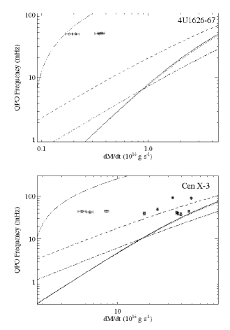
Figure 3: Predicted QPO frequencies in the BFM when the magnetospheric radius is calculated according to Eq. 20 (WM1, solid line), Eq. 21 (WM2, dashed line) Eq. 22 (WM3, dotted line), Eq. 23 (WM4, dash-dotted line), and Eq. 8 (GLM, triple-dot-dashed line). The upper panel is for 4U 1626-67, whereas the lower panel is for Cen X-3. In both cases QPO frequencies inferred from observations of these sources at different X-ray fluxes are shown together with measurement errors. These data taken from Kaur et al. (2008), Krauss et al. (2007), and Raichur & Paul (2008); we used Eq. 28 to convert between X-ray fluxes and mass accretion rates.

In this section we discuss further the cases of 4U 1626-67 and Cen X-3, for which detailed studies of the long term variations of the QPO frequency with the X-ray flux were recently published.

In particular, Kaur et al. (2008) studied QPOs in 4U 1626-67 at different X-ray fluxes and compared the observed frequencies with those calculated by using the BFM and with the magnetospheric radius determined based on the GLM. These authors noted a discrepancy between the observations and the predictions, and argued that the BFM might not apply to this source. In Fig 3 (upper panel) we show the same calculation, but included also the QPO frequencies estimated by using the BFM with the magnetospheric radius as determined in the WM. In this plot the solid line corresponds to the QPO frequency predicted by the BFM when Eq. 20 (WM1) is assumed for the magnetospheric radius, the dashed line is for Eq. 21 (WM2), dotted line for Eq. 22 (WM3), and the dash-dotted line for Eq. 23 (WM4). The triple-dot-dashed line represents the QPO frequencies predicted by the BFM when the magnetospheric radius is calculated according to the GLM (Eq. 8). We selected those data from Kaur et al. (2008) and Krauss et al. (2007) for which QPO frequencies and X-ray fluxes were measured simultaneously, and used Eq. 28 to convert these fluxes into mass accretion rates. In the upper panel of Fig. 3 we show that, due to the different prescriptions available for the magnetospheric radius (i.e. the GLM and the WM), the region of predicted QPO frequencies in the BFM, as a function of the mass accretion rate, is very broad and all observational measurements lie within this region.

The lower panel of Fig. 3 show the case of Cen X-3. We used data from Raichur & Paul (2008). In this work, the authors showed that the QPO frequency of this source has almost no dependence on the X-ray flux. By using the GLM to calculate the magnetospheric radius, they argued that, if the BFM applies, then the long term X-ray intensity variations of Cen X-3 are likely due to obscuration by an aperiodically precessing warped disk, rather than being related to changes in the mass accretion rate (and thus location of the inner disk radius). In fact, in the latter case the QPO frequency would be expected to vary according to Eqs. 27 and 4. However, our calculations show that all measured QPO frequencies lie inside the region spanned by different magnetically threaded disk models. We conclude that the observations of 4U 1626-67 and Cen X-3 do not support simple applications of either the GLM or WM to the BFM. We further comment on this in Sect. 5.

5 Discussion

The results obtained in the previous section indicate neither the GLM nor the WM, when used in conjunction with the BFM, are able to reproduce the range of observations discussed here for the entire sample of X-ray pulsars. We also note that for all sources in Fig. 2, the magnetospheric radius in the GLM turns out to be somewhat smaller than that derived by using the WM. This point was discussed also by Wang (1996), who suggested that the reason for this disagreement resides in the different prescription of the toroidal field used in the two models: the assumed $B_{\rm\phi}$ in the GLM implies a larger magnetic torque that spins down the NS more efficiently and reduces the value of the critical fastness parameter. As a consequence, the GLM magnetospheric radius is located closer to the NS (see Fig. 2). We showed here that the magnetospheric radius predicted by the GLM is still too large to account for observations of the QPOs over the entire sample of the slow rotators (see Table 1). This remains true even when the GLM is revised to include a more accurate prescription of the toroidal magnetic field, which leads to larger values of the critical fastness parameter (Wang, 1987; Ghosh & Lamb, 1992, 1995).

At odds with the GLM, the magnetospheric radius in the WM approaches the corotation radius more gradually as the mass accretion rate decreases, a result that seems to account for observations of fast rotating sources (see Table 1). However, in the cases of 4U 1626-67 and Cen X-3, for which detailed studies of the long term variations of the QPO frequency with the X-ray flux are available, the WM is not able to reproduce the observations. It was also noted that the treatment of the NS poloidal field screening by currents flowing onto the disk surface in this model might be oversimplified (Ghosh & Lamb, 1992, 1995).

Furthermore, in Sect. 2.2 we pointed out that an important caveat in the WM is that the interaction between the accretion disk and the NS magnetic field takes place in a similar fashion over the whole accretion disk. This is at odds with the GLM that predicts the strong coupling between the NS and the disk takes place mostly within a small boundary layer, such that this region alone determines the position where the disk terminates (i.e. $R_{\rm M}$). On the other hand, the theory of the boundary layer envisaged in the GLM might not be applicable to fast rotators, being the radial extent of the boundary layer of the same order of the separation between the magnetospheric and the corotation radii in these cases. Some works have investigated the importance of the boundary layer in the threaded disk model (Li & Wang, 1996; Li & Wickramasinghe, 1997; Li & Wang, 1999; Erkut & Alpar, 2004). Li & Wang (1996) suggested that there exists an uncertainty by a factor of 4 in the Wang (1987) equation defining the magnetospheric radius; using this result, Li & Wang (1999) demonstrated that the boundary layer in NS accreting binaries can survive the destructing action of the NS magnetic field down to a radius $\simeq$0.8$R_{\rm M}$. The boundary layer might thus be significantly larger than previously thought (Ghosh & Lamb, 1979a). However, the derived corrected value of the critical fastness parameter ($\sim$0.71-0.95) does not differ much from previous estimates (Wang, 1995) and the problem of slow rotating sources remains open. Similar results were obtained by Erkut & Alpar (2004), which demonstrated that the width of the boundary layer might be a strong function of the fastness parameter: they found that broad “boundary layers” are expected for spinning-up sources, whereas much reduced boundary layers should be expected for sources in a spin-down state (these boundary layers are typically a factor $\sim$6-60 less wider than those found for spinning-up sources). However, a general analytical equation for the magnetospheric radius cannot be easily derived, due to the presence of few additional parameters in their model. Broad boundary layers were found also in the simulations by Romanova et al. (2002). These authors found a reasonable agreement with the predictions of the GLM, with the inner region of the disk behaving like a boundary layer, while the outer region is only partially coupled with the magnetic field of the star. These numerical simulations suggested a critical fastness parameter of $\sim$0.6. Despite this value is in between the values obtained within the GLM and the WM, it cannot account for observations of both fast and slow rotators. Our results in Table 1 imply that the critical fastness parameter cannot be constant for all these sources. A more general solution for the magnetic threaded disk model might be found in the future in which the WM and the GLM give the limiting cases of fast and slow rotation, respectively.

The present study suggests that all the discussed limitations of both the WM and GLM might be the reason why none of these models is able to reproduce the combination of QPO and torque behaviour observed at different X-ray luminosity levels in the X-ray pulsars considered. Alternatively, the BFM might not be applicable to (all) QPOs observed from X-ray pulsars.

6 Conclusions

We showed that, if the BFM applies to the QPOs of X-ray pulsars, then the GLM and WM cannot completely account for observations of the sources in our sample. Instead, taking into accounts results in Table 1, we noted that these sources can be divided into two classes:

• Fast rotators, for which the Keplerian velocity of matter at the inner disk radius, as inferred from the application of the BFM to the observed QPO frequency, is close to the rotational velocity of the star. In this case, the magnetospheric radius inferred from the WM and the BFM predict QPO frequencies which seem in good agreement with the observations. However, we showed in Sect 4.1 that at least in the cases of 4U 1626-67 and Cen X-3, the WM is not able to reproduce observations of QPO frequencies at different X-ray fluxes.

• Slow rotators, for which the Keplerian velocity of matter at the inner disk radius, as inferred from the application of the BFM to the observed QPO frequency, is well above the spin velocity of the NS. In this case, the magnetospheric radius derived from the BFM is less discordant with the predictions of the GLM. In fact, only for A 0535+262 a good agreement between the GLM and the observations is obtained. For slow rotators the WM give a magnetospheric radius that is at least $\gtrsim$2-8 times larger than that derived from the BFM.

We conclude that either a more advanced theory of magnetically threaded disks is required, or that the BFM does not apply to (all) QPOs observed from X-ray pulsars.

Appendix A Calculation of the torque for region “C” of the SS73 accretion disk model

In order to evaluate $\rho$ and $h$ in Eqs. 9 and 12, Wang (1987) considered only the “B” region of the SS73 accretion disk, i.e. the gas-pressure dominated region where electron scattering gives the main contribution to the opacity. Here we carry out the same calculation by using the expressions of $\rho$ and $h$ that are appropriate to region “C” of the SS73 accretion disk model (where the main contribution to the opacity is provided by free-free absorption). According to Vietri (2008), the thermal pressure of disk matter has a radial dependence $p=p_{\rm M}(R_{\rm M}/R)^{21/8}$, where the subscript $M$ denotes quantities evaluated at the inner disk radius. From Eq. 9 we get

$$\left|B_{\phi}(R)\right| = B_{\phi 0}\frac{\omega_{\rm s}^{23/16}}{|1-\omega_{\rm s}|^{1/2}}\left(\frac{R_{\rm co}}{R}\right)^{69/32}\cdot$$

$$\cdot\left|1-\left(\frac{R}{R_{\rm co}}\right)^{3/2}\right|^{1/2},$$

where the same notation as that of Sect. 2 is used. Setting $y=(R/R_{\rm co})^{3/2}$ and using Eq. A into Eq. 12 we obtain

$$n(\omega_{\rm s}) = 1+\frac{1}{3}\frac{\omega_{\rm s}^{23/16}}{|1-\omega_{\rm s}|^{1/2}}\cdot$$

$$\cdot\left[\int_{\omega}^{1}\frac{(1-y)^{1/2}}{y^{39/16}}dy-\int_{1}^{\infty}\frac{(y-1)^{1/2}}{y^{39/16}}dy\right].$$

By numerically evaluating integrals in the above equation we find $\omega_{c}=0.95$.

Appendix B Values of $L_{\rm tr}$ and $L_{\rm QPO}$ for accretion powered X-ray sources

Here we briefly summarize the relevant observations of the accretion powered X-ray pulsars considered in Table 1, in order to explain values used for the luminosities $L_{\rm tr}$ and $L_{\rm QPO}$.

• Her X-1: Her X-1 is one of the best studied X-ray binary system. It consists of a $\sim$1.24 s spinning NS and a A/F companion (the orbital period is 1.7 day). The X-ray flux displays a regular modulation at a 35 day period, that has been associated to the precession of a highly warped accretion disk that periodically obscures the NS (Petterson, 1975; Choi et al., 1994; Wilson et al., 1997; Dal Fiume et al., 1998; Parmar et al., 1999; Klochkov et al., 2007). This suggested that transitions between high (“main-on states”) and low luminosity states (the “anomalous” low states) of this source are to be interpreted as due to local obscuration phenomena, rather than large changes in the mass accretion rate. Evidence in favor of this interpretation has been recently obtained through detailed phase-resolved spectroscopy (Zane et al., 2004) as well as observations of X-ray heating of the companion star (Boroson et al., 2000). Since QPOs and spin-up/spin-down transitions were observed during both high and low luminosity states, for the purpose of this paper we assume $L_{\rm tr}$=$L_{\rm QPO}$=2.1$\times$10³⁷ erg s^-1 (a distance of 5 kpc is considered), where the latter is the typical main-on state luminosity.

• 4U 0115+63: 4U 0115+63 is a binary system hosting a 3.6 s spinning NS orbiting a Be companion (the orbital period is 24.3 day). The distance to the source is $\sim$8 kpc (Negueruela & Okazaki, 2001). An HEAO observation caught this source in outburst (the typical outburst luminosity is $\sim$8$\times$10³⁷ erg s^-1, , 2001), and a prominent peak in the power spectrum of the X-ray light curve was detected at 62 mHz (Soong & Swank, 1989). Tamura et al. (1992) reported that the spin-up trend the source usually displayed while in outbursts reversed during lower luminosity states. These typically occurred at 5$\times$10³⁵ erg s^-1 (, 2001).

• Cen X-3: Cen X-3 is a high mass X-ray binary with a spin period of $\sim$4.8 s and an orbital period of $\sim$2.1 day. The companion star is an O-type supergiant and the distance is estimated to be $\sim$8 kpc (Burderi et al., 2000, and references therein). The presence of a $\sim$35 mHz QPO in the power spectrum of this source was first discovered by Takeshima et al. (1991), after the source egress from an X-ray eclipse. The typical X-ray luminosity was determined with BeppoSAX, and is of order $\sim$1.0$\times$10³⁸ erg s^-1 (0.12-100 keV). Cen X-3 has a secular spin-down trend (Bildsten et al., 1997), but episodes of spin reversal were found to occur at a luminosity that is typically a factor of $\sim$3 below that of the post-eclipse high luminosity state (Howe et al., 1983). We thus considered in Table 1 that $L_{\rm QPO}$ is equal to the typical X-ray luminosity observed in the post-eclipse egress state, whereas $L_{\rm tr}$$\sim$1/3$L_{\rm QPO}$.

• LMC X-4: LMC X-4 is an accretion powered X-ray pulsar with a spin period of $\sim$13.5 s and an orbital period of $\sim$1.4 day. The X-ray luminosity of the system varies with a periodicity of $\sim$30.3 day, alternating between high ($\sim$2$\times$10³⁸ erg s^-1) and low (a factor of $\sim$60 below) luminosity states (for an estimated distance of $\sim$50 kpc, Woo et al., 1996). This periodicity have been attributed to the effect of an obscuring tilted accretion disk (Moon & Eikenberry, 2001b, and references therein). During the high states, spin torque reversals were repeatedly observed, whereas during episodes of very bright flares ($\sim$10³⁹ erg s^-1, 2-25 keV) QPOs were detected at frequencies in the $\sim$0.65-1.35 mHz range (these were interpreted within the BFM by Moon & Eikenberry, 2001b).

• 4U 1626-67: 4U 1626-67 is a low mass X-ray binary hosting a $\sim$7.7 s spinning neutron star in a $\sim$42 min orbit around a $\sim$0.004 M_⊙ companion star. QPOs were detected in the X-ray observations of this source more than once (for a review see, e.g. Kaur et al., 2008). A torque reversal was observed by Chakrabarty et al. (1997), who also estimated a source distance of $\sim$3 kpc. For a review of the flux history of 4U 1626-67, we reefer the reader to Krauss et al. (2007).

• EXO 2030+375: EXO 2030+375 is a Be X-ray transient with an orbital period of $\sim$46 day, hosting a $\sim$42 s spinning neutron star, and located at a distance of 7.1 kpc (Wilson et al., 2002). In 1985 this source underwent a bright outburst (peak luminosity $\sim$2$\times$10³⁸ erg s^-1), and a QPO at $\sim$213 mHz was detected (Angelini et al., 1989). Spin-up/spin-down transitions were observed more than once, at luminosities in the $\sim$10³⁸-2.4$\times$10³⁶ erg s^-1 (1-20 keV) range.

• A0535+262: A0535+262 is a $\sim$103 s X-ray pulsar, orbiting a O9.7 companion star (the orbital period is $\sim$111 day). QPOs and spin reversals were best observed during the giant outburst in 1994 (Finger et al., 1996). This outburst was detected with BATSE in the energy 20-100 keV range, and the flux at the peak of the outburst was $\sim$6 Crab. Observations of this outburst at lower energies ($<$20 keV) were not available, but, based on previous results, Finger et al. (1996) estimated the 2-10 keV flux might not be larger than 2 Crab. Due to the uncertainties in this estimate we have not corrected values reported in Table 1 for this factor. As discussed in Sect. 4 an uncertainty of $\sim$30% on the luminosity used to derive the position of the magnetospheric radius cannot affect much our results. Note that the distance used by Finger et al. (1996) to convert the observed flux into an X-ray luminosity is 2 kpc (Steele et al., 1998).

• 4U 1907+09: 4U 1907+09 is a $\sim$440 s spinning NS in a $\sim$8 day orbit around a supergiant companion. QPOs were discovered during an hour long flare at $\sim$6.3$\times$10³⁶ erg s^-1 (2-60 keV, and an assumed distance of 5 kpc, in’t Zand et al., 1998; Cox et al., 2005). After the discovery of the pulsations by Makishima et al. (1992), the NS in 4U 1907+09 exhibited a steady spin-down for about 20 yrs. This trend changed in 2006, when a torque reversal was observed at $\sim$2$\times$10³⁶ erg s^-1 (1-15 keV, Fritz et al., 2006).

References

- Alpar et al. (1985) Alpar, M.A., Shaham, J. 1985, Nature, 316, 239
- Angelini et al. (1989) Angelini, L., Stella, L., Parmar, A.N. 1989, ApJ, 346, 906
- Bildsten et al. (1997) Bildsten, Lars, Chakrabarty, D., Chiu, J., et al. 1997, ApJs, 113, 367
- Boroson et al. (2000) Boroson, B., O’Brien, K., Horne, K., Kallman, T., Still, M., Boyd, P.T., Quaintrell, H., Vrtilek, S.D. 2000, ApJ, 545, 399
- Burderi et al. (2000) Burderi, L., Di Salvo, T., Robba, N.R., La Barbera, A., Guainazzi, M. 2000, ApJ, 530, 429
- (6) Campana, S., Gastaldello, F., Stella, L., et al. 2001, ApJ, 561, 924
- Chakrabarty et al. (1997) Chakrabarty, D., Bildsten, L., Grunsfeld, J.M. 1997 ApJ, 474, 414
- Chakrabarty (1998) Chakrabarty, D. 1998, ApJ, 492, 342
- Choi et al. (1994) Choi, C.S., Nagase, F., Makino, F., Dotani, T., Min, K.W. 1994, ApJ, 422, 799
- Cox et al. (2005) Cox, N.L.J., Kaper, L., Foing, B.H., Ehrenfreund, P. 2005, A&A, 438, 187
- Dal Fiume et al. (1998) dal Fiume, D., Orlandini, M., Cusumano, G., del Sordo, S., Feroci, M., Frontera, F., Oosterbroek, T., Palazzi, E., Parmar, A.N., Santangelo, A., Segreto, A. 1998, A&A, 329 L41
- Erkut & Alpar (2004) Erkut, M.H., Alpar, M.A. 2004, ApJ, 617, 461
- Finger et al. (1996) Finger, M.H., Wilson, R.B., Harmon, B.A. 1996, ApJ, 459, 288
- Fritz et al. (2006) Fritz, S., Kreykenbohm, I., Wilms, J., Staubert, R., Bayazit, F., Pottschmidt, K., Rodriguez, J., Santangelo, A. 2006, A&A, 458, 885
- Ghosh et al. (1977) Ghosh, P., Pethick, C. J., Lamb, F. K. 1977, ApJ, 217, 578
- Ghosh & Lamb (1978) Ghosh, P., Lamb, F.K. 1978, ApJ, 223, L83
- Ghosh & Lamb (1979a) Ghosh, P., Lamb, F. K. 1979a, ApJ, 232, 259
- Ghosh & Lamb (1979b) Ghosh, P., Lamb, F. K. 1979b, ApJ, 234, 296
- Ghosh & Lamb (1992) Ghosh, P.; Lamb, F. K. 1992, in X-ray binaries and recycled pulsars, Ed. E. van den Heuvel and S.A. Rappaport (Kluwer Academic Publishers, Boston), p. 487
- Ghosh & Lamb (1995) Ghosh, P.; Lamb, F. K. 1995, in Compact stars in binaries, Ed. J. van Paradijs, E.P.J. van den Heuvel, E. Kuulkers ù (Kluwer Academic Publishers, Dordrecht), p.57
- Howe et al. (1983) Howe S.K., Primini, F.A., Bautz, M.W., et al, 1983, ApJ, 272, 678
- in’t Zand et al. (1998) in’t Zand, J.J.M., Baykal, A., Strohmayer, T.E. 1998, ApJ, 496, 386
- Kaur et al. (2008) Kaur, R., Paul, B., Kumar, B., Sagar, R. 2008, ApJ, 676, 1184
- King et al. (2007) King, A.R., Pringle, J.E., Livio, M. 2007, MNRAS, 376, 1740
- van der Klis (1995) van der Klis, M. 1995, in X-Ray Binaries, 252
- van der Klis (2004) van der Klis, M. 2004, arXiv:astro-ph/0410551
- Klochkov et al. (2007) Klochkov, D., Shakura, N., Postnov, K., Staubert, R., Wilms, J., Ketsaris, N. 2006, arXiv:astro-ph/0609276
- Krauss et al. (2007) Krauss, M.I., Schulz, N.S., Chakrabarty, D., Juett, A.M., Cottam, J. 2007, ApJ, 660, 605
- Lamb & Pethick (1974) Lamb, F.K., Pethick, C.J. 1974, in Astrophysics and gravitation; Proceedings of the Sixteenth Solvay Conference on Physics, Brussels, Belgium, Editions de l’Universite de Bruxelles 1974, p. 135-141.
- Lamb et al. (1985) Lamb, F.K., Shibazaki, N., Alpar, M.A., Shaham, J. 1985, Nature, 317, 681
- Li & Wang (1996) Li, X.-D., Wang, Z.-R. 1996, A&A, 307, L5
- Li & Wang (1999) Li, X.-D., Wang, Z.-R. 1999, ApJ, 513, 845
- Li et al. (1996) Li, J., Wickramasinghe, D.T., Rudinger, G. 1996, MNRAS, 469, 765
- Li & Wickramasinghe (1997) Li, J., Wickramasinghe, D.T. 1997, MNRAS, 286, L25
- Lovelace et al. (1995) Lovelace, R. V. E., Romanova, M. M., Bisnovatyi-Kogan, G. S. 1995, MNRAS, 244, 254
- Makishima et al. (1992) Makishima, K., Mihara, T., Nagase, F., Murakami, T. 1992, in Proc. 28th Yamada Conference: Frontiers of X-ray Astronomy, ed. Y. Tanaka & K. Koyama, Frontiers Science Series (Tokyo: Universal Academy Press), 23
- Moon & Eikenberry (2001a) Moon, D., Eikenberry, S.S. 2001, ApJ, 549, L225
- Moon & Eikenberry (2001b) Moon, D., Eikenberry, S.S. 2001, ApJ, 552, L135
- Negueruela & Okazaki (2001) Negueruela, I. & Okazaki, A.T. 2001, A&A, 369, 108
- Parmar et al. (1989) Parmar, A.N., White, N.E., Stella, L. 1989, ApJ, 338, 373
- Parmar et al. (1999) Parmar, A.N., Oosterbroek, T., Dal Fiume, D., et al. 1999, A&A, 350, L5
- Petterson (1975) Petterson, J.A. 1975, ApJ, 201, L61
- Raichur & Paul (2008) Raichur, H. & Paul, B. 2008, preprint (astro-ph/0806.0949)
- Romanova et al. (2002) Romanova, M.M., Ustyugova, G.V., Koldoba, A.V., Lovelace, R.V.E. 2002, ApJ, 578, 420
- Romanova et al. (2003) Romanova, M.M., Ustyugova, G.V., Koldoba, A.V., Wick, J.V., Lovelace, R.V.E. 2003, ApJ, 595, 1009
- Romanova et al. (2004) Romanova M.M., Ustyugova G.V., Koldoba A.V., Lovelace R.V.E. 2004, ApJ, 616, L151
- Scharlemann (1978) Scharlemann, E.T. 1978, ApJ, 219, 617
- Shakura & Sunyaev (1973) Shakura, N.I., Sunyaev, R.A. 1973, A&A, 24, 337
- Shinoda et al. (1990) Shinoda, K., Kii, T., Mitsuda, K., et al 1990, PASj, 42, L27
- Soong & Swank (1989) Soong, Y. & Swank, J.H. 1989, in X Ray Binaries, the 23rd ESLAB Symposium on Two Topics in X Ray Astronomy, p. 617
- Steele et al. (1998) Steele, I.A., Negueruela,I., Coe, M.J., Roche, P. 1998, MNRAS, 297, L5
- Takeshima et al. (1991) Takeshima T., Dotani, T., Mitsuda, K., Naga, F. 1991, PASJ, 43, L43
- Tamura et al. (1992) Tamura, K., Hiroshi, T., Kitamoto, S., et al. 1992, ApJ, 389, 676
- Ustyugova et al. (2006) Ustyugova, G. V.; Koldoba, A. V.; Romanova, M. M.; Lovelace, R. V. E.
- Vietri (2008) Vietri, M. 2008, Foundations of high-energy astrophysics, Chicago University press, pp. 325
- Wang (1987) Wang, Y.-M. 1987, A&A, 183, 257
- Wang (1995) Wang, Y.-M. 1995, ApJ, 449, L153
- Wang (1996) Wang, Y.-M. 1996, ApJ, 465, L111
- Wang (1997) Wang, Y.-M. 1997, ApJ, 475, L135
- Wang (1997b) Wang, Y.-M. 1997, ApJ, 487, L85
- Wilson et al. (1997) Wilson, R.B., Scott, D.M., Finger, M.H. 1997, AIP Conf. Proc., 410, 739
- Wilson et al. (2002) Wilson, C.A., Finger, M.H., Coe, M.J., Laycock, S., Fabregat, J. 2002, ApJ, 570, 287
- Woo et al. (1996) Woo, J.W., Clark, G.W., Levine A.M., et al. 1996, ApJ, 467, 811
- Zane et al. (2004) Zane, S., Ramsay, G., Jimenez-Garate, M.A., Willem den Herder, J., Hailey, C.J. 2004, MNRAS, 350, 506