Magnetoresistance in Spin-Polarized Transport through a Carbon Nanotube

Abstract

We report on our theoretical study of the magnetoresistance in spin polarized transport through a finite carbon nanotube (CNT). Varying the Fermi energy of a CNT and the relative strength of couplings to two ferromagnetic (FM) electrodes, we studied the conductance as well as the magnetoresistance (MR). Due to resonant transport through discrete energy levels in a finite CNT, the conductance and MR are oscillating as a function of the CNT Fermi energy. The MR is peaked at the conductance valleys and dipped close to the conductance peaks. When couplings to two FM electrodes are asymmetric, the MR dips become negative under a rather strong asymmetry. When couplings are more or less symmetric, the MR dips remain positive except for a very strong coupling case. Under strong coupling case, the line broadening is significant and transport channels through neighboring energy levels in a CNT interfere with each other, leading to the negative MR.

I Introduction

Spin-polarized transport review has attracted lots of attention because of its potential applications to spintronic devices. Spintronics attempts to use the electron spin in order to control the electric current in the devices. The spin valve, consisting of a non-magnetic (NM) material sandwiched in between two ferromagnetic (FM) electrodes, is a typical two-terminal spintronic device. The current in the spin valve is modulated by the relative orientation of magnetizations in the two FM electrodes. Usually more current flows when the two magnetizations are parallel than when they are antiparallel. The difference in resistance between two configurations of magnetization is called the magnetoresistance (MR).

In addition to the relative orientation of magnetizations, there are many other methods to control the current in the spin valve systems. In magnetic tunnel junctions (MTJs), the oxide barriers can change the tunneling magnetoresistance (TMR) in a significant way. With MgO barrier, TMR values reaching several hundred percents were predicted theoretically the_mgo and reported experimentally. exp_mgo The MgO layer acts as the highly spin selective filter. The sign of TMR can be changed with different oxide barriers. For example, tunneling through Al oxide barriers is dominated by $s$ electrons leading to normal positive TMR. On the other hand, the $d$ electrons can tunnel SrTiO₃ barriers sto more easily with the negative or inverse TMR. The oxidation process of the insulating barriers also affects the TMR values. Strongly temperature dependent suppression of TMR was reported mtjkondo for MTJs with heavily oxidized Al oxide barriers. Inclusion of the dusting layers dustlayer in the MTJs changes the TMR values, too.

The current in the spin valve can also be modulated by the third electrode which is coupled capacitively to the non-magnetic material. Though the three-terminal spintronic device or the spin field-effect transistor (FET) was suggested theoretically, datta it was not realized experimentally as yet. To implement the gate electrode into the spin valve tends to lengthen naturally the nonmagnetic part. The success of the spin FET seems to depend on the efficient spin injection from the FM electrode into the NM part and the preservation of the spin coherence in the NM part. Due to the low atomic number of carbon and accordingly the weak spin-orbit interaction in carbon systems, the CNT and graphene are considered as ideal candidates for the NM part in the spin valves. The CNTs and graphenes are featured with a very long spin-diffusion length (up to a few $\mu$m) and spin-flip time (up to a few tens of ns) at room temperature.

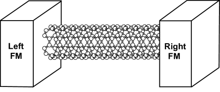
Figure 1: Schematic display of a carbon nanotube (CNT) system. The finite CNT consists of $N$ layers and is end-contacted to the left and right ferromagnetic electrodes.

There have been several experimental attempts to measure the MR in the spin valves with the CNTs, svalve_CNT1 ; svalve_CNT2 ; svalve_CNT3 ; svalve_CNT4 ; high_MR_cnt ; omr_cnt1 ; omr_cnt2 ; imr_cnt the graphenes, svalve_CG1 ; svalve_CG2 ; svalve_CG3 ; svalve_CG4 and the fullerenes (C60). svalve_C60a ; svalve_C60b For the spin valves with the CNT, the positive MR svalve_CNT1 ; high_MR_cnt as well as negative MR imr_cnt were reported. The inverse MR (up to 6 %) was observed imr_cnt in the Co/CNT/Co and Co/CNT/Ni spin valves with a highly transmissive contact. On the other hand, the positive 61 % MR is observed high_MR_cnt in the CNT spin valves with the half-metal electrode (tunneling contact). More interestingly, some experimental groups omr_cnt1 ; omr_cnt2 succeeded in modulating the MR in the CNT spin valves (NiPd electrodes) with the gate electrode. The observed MR and conductance are correlated and oscillating as a function of the gate voltage. The MR is positive and peaked in the conductance valleys, while it is suppressed and becomes even negative near the conductance peaks. The control of the MR and conductance with the gate voltage suggests that the resonant tunneling through quantized energy levels in a finite CNT is responsible for the spin-polarized transport.

Some experimental features can be understood in terms of the spin-polarized transport through a single resonant level. itmr_tsymbal Suppose that one energy level with energy $\epsilon_{0}$ is coupled to two source and drain (left and right) ferromagnetic electrodes. The transmission probability for an electron with spin direction $\alpha=\pm$ (spin-up/spin-down) from one electrode to the other is given by the expression at the Fermi level in the linear regime

$$T_{\alpha}(0) = \frac{4\Gamma_{L\alpha}\Gamma_{R\alpha}}{\epsilon_{0}^{2}+(\Gamma_{L\alpha}+\Gamma_{R\alpha})^{2}}.$$ (1)

$\epsilon_{0}$ can be adjusted by the gate voltage. $\Gamma_{p\alpha}$ is the spin-dependent linewidth of a resonant level coming from the coupling to the $p=L,R$ (left and right) electrode. The magnetoresistance is dependent sensitively on the position of $\epsilon_{0}$ relative to the Fermi level in the electrodes. Close to or on resonance ($\epsilon_{0}=0$), the transmission probability is simplified as

$$T_{\alpha} = \frac{4\Gamma_{L\alpha}\Gamma_{R\alpha}}{(\Gamma_{L\alpha}+\Gamma_{R\alpha})^{2}}.$$ (2)

For highly asymmetric coupling to two electrodes, say, $\Gamma_{L}\gg\Gamma_{R}$, the transmission probability is simplified as

$$T_{\alpha} \simeq \frac{4\Gamma_{R\alpha}}{\Gamma_{L\alpha}},$$ (3)

and the MR ratio can be obtained as

MR $$= \frac{G_{P}-G_{AP}}{G_{AP}}~{}=~{}-\frac{2\beta_{L}\beta_{R}}{1+\beta_{L}\beta_{R}}.$$ (4)

The inverse or negative MR is obtained for a highly asymmetric coupling case. Here $G_{P}$ and $G_{AP}$ are the conductance in the spin valve for the parallel and antiparallel configurations of magnetizations, respectively. The spin polarization $\beta_{p}$ in the linewidth is defined by the relation $\Gamma_{p\pm}=\Gamma_{p}(1\pm\beta_{p})$, where $p=L,R$ denotes the left and right electrode.

Off resonance or when the Fermi level is far away from the resonant level, the transmission probability can be simplified as

$$T_{\alpha} \simeq \frac{4\Gamma_{L\alpha}\Gamma_{R\alpha}}{\epsilon_{0}^{2}}.$$ (5)

This approximation gets better with the smaller linewidth. The MR ratio can be readily computed from this approximation.

MR $$= \frac{2\beta_{L}\beta_{R}}{1-\beta_{L}\beta_{R}}.$$ (6)

This expression of MR is similar to that for the Julliere model of the magnetic tunnel junction (MTJ). From this simple resonant level model, we can deduce that the MR is bounded roughly by two values of Eqs. (4) and (6). The MR is dipped at the value of Eq. (4) near the conductance peaks and is peaked at the value of Eq. (6) at the conductance valleys. Though some features of experimental MR can be understood based on a single resonant level model, we shall show in this work that the interference between multi quantized energy levels in a finite CNT plays an important role in the spin-polarized transport.

In this paper we study theoretically the magnetoresistance in the phase-coherent spin-polarized transport through a finite carbon nanotube (CNT). Our model system, schematically shown in Fig. 1, is a typical spin valve with a carbon nanotube sandwiched in between two (left and right) FM electrodes. In addition, the carbon nanotube is coupled capacitively to a gate electrode such that the energy levels or the Fermi energy in a CNT can be shifted up and down by the gate voltage. In our model study, the control parameters are the Fermi energy level in a CNT (or the gate voltage) as well as the relative strength of coupling constants between a CNT and two FM electrodes. The linear conductance as well as MR are oscillating as a function of the CNT Fermi energy. The MR is featured with a peak in the conductance valleys and a dip structure near the conductance peaks. The shape of MR as a function of the gate voltage depends on the relative magnitude of couplings to the left and right FM electrodes. (1) With asymmetric couplings to the two FM electrodes, the MR dips become negative under a high asymmetric aspect ratio of couplings. When the coupling strength is increased, the (negative) MR dip structure is broadened. (2) For symmetric couplings, qualitatively different behavior is observed in MR depending on the coupling strength. In the case of weak couplings, the MR as a function of the gate voltage is oscillating without any sign change. The simple peak appears in the conductance valleys, but the positive dip near the conductance peaks has an additional local peak, that is, a dip-peak-dip structure. When the coupling strength is increased, discrete energy levels in a CNT are broadened and overlap each other. Due to the interference between neighboring energy levels, the dip now becomes negative and the MR shape is highly asymmetric with respect to the peak position. One remarkable point is that the inverse MR in resonant transport can be observed for the case of symmetric strong couplings or for the highly transmissive contact between CNT and the FM electrode. Our study suggests another way to change the MR values by controlling the coupling between FM electrodes and a finite CNT. Our study can be equally applied to other nanostructures where discrete energy levels are formed due to their finite size. The preliminary results of our work is already reported elsewhere. mr_cnt_kll

The rest of this paper is organized as follows. In Sec. II, the model Hamiltonian is introduced for the FM-CNT-FM system and the spin-polarized current is formulated in a Landauer-Büttiker form. The results of our work are presented in Sec. III and a conclusion is included in Sec. IV. In Appendix A, we present the tight-binding Hamiltonian approach to a CNT and the phase information about the $\pi$ and $\pi^{*}$ states. In Appendices B and C, we elaborate on the coupling matrix between the CNT and the ferromagnetic electrodes and discuss its symmetry.

II Formalism

To study the phase-coherent spin-polarized transport through a carbon nanotube, we consider the model system which is schematically displayed in Fig. 1. The finite armchair-type $(n,n)$ carbon nanotube (CNT) is end-contacted to the two ferromagnetic electrodes. The band structure of the metallic CNTs close to the Fermi level Blase is known to be described accurately by the single $\pi$ electron tight-binding Hamiltonian

$$H_{cnt} = \sum_{i\alpha}\epsilon_{g}a_{i\alpha}^{{\dagger}}a_{i\alpha}-t\sum_{<i,j>}\sum_{\alpha}\left(a_{i\alpha}^{{\dagger}}a_{j\alpha}+h.c.\right)$$ (7)

$$= \sum_{\alpha}\Psi_{\alpha}^{{\dagger}}{\cal H}_{cnt}\Psi_{\alpha}.$$

Here $i,j$ runs through the atomic carbon sites in CNT and $<i,j>$ denotes the nearest neighbor pairs. $\alpha=\pm$ represents two spin directions, up ($+$) and down ($-$), and the hopping integral $t=2.66$ eV. Blase The on-site energy $\epsilon_{g}$ at each carbon site is proportional to the gate bias voltage and is chosen to be zero in the absence of the gate bias. Strictly speaking, the on-site energy at each carbon site depends on the separation of each site from the substrate (which is capacitively coupled to the gate electrode). In this work, we ignore such dependence and assume the on-site energy to shift uniformly by the gate voltage. In the second line, $H_{cnt}$ is written in a matrix form, where ${\cal H}_{cnt}$ is the square matrix and reflects the structure of the tight-binding Hamiltonian in the $(n,n)$ CNT. $\Psi_{\alpha}$ is the electron annihilation operator represented by the column vector and has as many components as the number of atomic sites in the finite CNT.

The $(n,n)$ CNT has the discrete rotational axial symmetry $C_{nv}$ about its axis. For details, look at Appendices A and C. The energy bands in a CNT can be classified using the group representation. Since the energy dispersion is a function of wave vector along the nanotube axis, every energy band can be uniquely specified by the quantum number belonging to the irreducible representations. There are in total $4n$ bands for the $(n,n)$ carbon nanotubes out of which four bands are nondegenerate and other $2n-2$ bands are doubly degenerate. The nondegenerate four bands are named as $\pi$ and $\pi^{*}$ bands (two $\pi$ and two $\pi^{*}$ bands). Out of these four bands, only two ($\pi$ and $\pi^{*}$ bands) cross the Fermi level ($E_{F}$). Only these $\pi$ and $\pi^{*}$ bands, crossing the Fermi level, are relevant to our spin polarized transport study. All other bands are gapped close to the Fermi energy.

In finite $(n,n)$ CNTs with $N$ layers, the discrete energy levels close to $E_{F}$ of $\pi$ (bonding) and $\pi^{*}$ (antibonding) characters will provide the transport channels for electrons incident from the ferromagnetic electrode. Outside this energy window, other higher-lying bands start to contribute to the electronic transport. The $\pi$ states are featured with no change in the relative phase from one carbon site to the other along the circumference in one layer. On the other hand, the $\pi^{*}$ states have the alternating relative phase, $+1$ and $-1$. For details, look at Appendix A.

The left ($p=L$) and right ($p=R$) FM metals are described by the two conduction bands of majority and minority spins.

$$H_{cb} = \sum_{p=L,R}\sum_{\vec{k}\alpha}\epsilon_{p\vec{k}\alpha}c_{p\vec{k}\alpha}^{{\dagger}}c_{p\vec{k}\alpha}.$$ (8)

Here $c_{p\vec{k}\alpha}^{{\dagger}}$ and $c_{p\vec{k}\alpha}$ are the creation and annihilation operators, respectively, for electrons of wave vector $\vec{k}$ in the electrode $p=L,R$, with the spin direction $\alpha=\pm$. $\alpha=+(-)$ means the spin is aligned parallel (antiparallel) to the direction of magnetization. $\epsilon_{p\vec{k}\alpha}$ is the energy dispersion relation for electrons in the ferromagnetic metals.

The coupling between a CNT and the electrodes is neither well controlled experimentally nor well understood theoretically yet. In one theoretical paper jihm only the $\pi^{*}$ states are coupled to the electrode of a jellium model and the $\pi$ states are effectively decoupled. In other theoretical work,pi_pistar the $\pi$ ($\pi^{*}$) states are strongly (weakly) coupled to the Al electrodes for the end-contact geometry. In this paper we are going to adopt the symmetry-adapted coupling based on the group theory and confine our interest to one specific end-contact geometry. For the end-contact geometry, only the carbon atoms at the left and right edge layers are assumed to be coupled to the FM electrodes. This coupling Hamiltonian can be written as kimcox

$$H_{1} = \sum_{p\vec{k}\alpha}\sum_{j}c_{p\vec{k}\alpha}^{{\dagger}}\langle p\vec{k}\alpha|V|j\alpha\rangle a_{j\alpha}+H.c.$$ (9)

$V$ is the coupling Hamiltonian between the CNT and FM electrodes and assumed to be spin-conserving. The coupling can be dependent on the electron spin direction.

In order to find the electric current we need to rewrite the model Hamiltonian in the symmetry-adapted basis. From here on, without loss of any generality we focus our discussion on the $(5,5)$ CNT. We can define the angular momentum $m$ about the nanotube axis for electronic states in a CNT as well as in the FM electrodes. However the angular momentum states $e^{im\phi}$ ($m$ is an integer) are not the basis functions of the symmetry group of the $(5,5)$ CNT. As discussed in Appendix C, the $\pi$ ($\pi^{*}$) states belong to the $A_{1}$ ($A_{2}$) irreducible representation (irred. rep.), respectively. The basis functions of $A_{1}$ irred. rep. are $\cos(5m\phi)$ with nonnegative integer $m$ and those of $A_{2}$ irred. rep. are $\sin(5m\phi)$ with positive integer $m$. The spin polarized electrons should have the wave functions with angular dependence of $\cos 5m\phi$ ($\sin 5m\phi$) in order to tunnel resonantly through the $\pi$ ($\pi^{*}$) states of the $(5,5)$ CNT, respectively.

We project the electron states of the ferromagnetic electrodes based on the irred. reps. of the $(5,5)$ CNT and keep only the states belonging to the $A_{1}$ and $A_{2}$ irred. reps. Other projected states belonging to $E_{1}$ and $E_{2}$ representations are not coupled to the $\pi$ and $\pi^{*}$ states of the $(5,5)$ CNT.

$$H_{1} = \sum_{\vec{k}}\sum_{pj\alpha}c_{p\vec{k}\alpha}^{{\dagger}}\langle p\vec{k}\alpha|V|j\alpha\rangle a_{j\alpha}+H.c.$$ (10)

$$= \sum_{k_{z}k_{\perp}}\sum_{m=-\infty}^{\infty}\sum_{pj\alpha}c_{pk_{z}k_{\perp}m\alpha}^{{\dagger}}\langle pk_{z}k_{\perp}m\alpha|V|j\alpha\rangle a_{j\alpha}$$

$$+H.c.$$

Here we note that $\vec{k}=k_{z}\hat{z}+\vec{k}_{\perp}$ and $k_{\perp}=|\vec{k}_{\perp}|$. The azimuthal angle dependence can be written down explicitly as

$$\langle pk_{z}k_{\perp}m\alpha|V|j\alpha\rangle = V_{pm\alpha}(k_{z},k_{\perp})e^{im\phi_{j}}.$$ (11)

Here $\phi_{j}$ represents the angular position of the $j$-th carbon atom along the circumference of the edge layer. The angle is measured from any line which intersects the tube axis perpendicularly and bisects two neighboring carbon atoms at the edge layer. For example, $\phi_{j}$ takes the following set of values for $(5,5)$ CNT, alternating between the odd-th and even-th layers.

$$\{\phi_{j}\} = \frac{2\pi}{5}\left\{\pm\frac{1}{6},1\pm\frac{1}{6},2\pm\frac{1}{6},3\pm\frac{1}{6},4\pm\frac{1}{6}\right\},$$ (12)

$$= \frac{2\pi}{5}\left\{\pm\frac{1}{3},1\pm\frac{1}{3},2\pm\frac{1}{3},3\pm\frac{1}{3},4\pm\frac{1}{3}\right\}.$$

We need to consider only those angular momentum states $m$ which are multiples of $5$ for the $(5,5)$ CNT system.

$$H_{1} = \sum_{k_{z}k_{\perp}}\sum_{m=-\infty}^{\infty}\sum_{pj\alpha}c_{pk_{z}k_{\perp}5m\alpha}^{{\dagger}}V_{p5m\alpha}(k_{z},k_{\perp})e^{i5m\phi_{j}}a_{j\alpha}$$ (13)

$$+H.c.$$

Rearranging terms in the basis functions of the $A_{1}$ and $A_{2}$ irreducible representations, the relevant coupling Hamiltonian can be written down as $H_{1}=H_{1\pi}+H_{1\pi^{*}}$.

$$H_{1\pi} = \sum_{k_{z}k_{\perp}}\sum_{m=0}^{\infty}\sum_{pj\alpha}\left[c_{p\pi k_{z}k_{\perp}m\alpha}^{{\dagger}}V_{p\pi m\alpha}(k_{z},k_{\perp})\cos(5m\phi_{j})a_{j\alpha}+H.c.\right],$$ (14a)

$$H_{1\pi^{*}} = \sum_{k_{z}k_{\perp}}\sum_{m=1}^{\infty}\sum_{pj\alpha}\left[c_{p\pi^{*}k_{z}k_{\perp}m\alpha}^{{\dagger}}V_{p\pi^{*}m\alpha}(k_{z},k_{\perp})\sin(5m\phi_{j})a_{j\alpha}+H.c.\right].$$ (14b)

In our model study, two projected $\pi$ and $\pi^{*}$ bands contribute to the electronic transport independently. Each band has mutually independent infinite number of transport channels (indexed by $m$). For angular position $\phi_{j}$ given by Eq. (12), $\cos(5m\phi_{j})$ is independent of $j$ while $\sin(5m\phi_{j})\propto(-1)^{j}$. That is to say, the projected $\pi$ and $\pi^{*}$ conduction bands correctly pick up the $\pi$ and $\pi^{*}$ states in the CNT, respectively.

According to the above analysis based upon the symmetry, the $\pi$ and $\pi^{*}$ states are characterized by the following properties: (i) All carbon atoms at the edge layer are coupled to the electrode with the same magnitude of coupling constants; (ii) The coupling constants are uniform in phase for the $\pi$ states, but alternating in sign from one atom to the other for the $\pi^{*}$ states. These properties are true for all projected bands in the electrode. We can introduce the following effective model Hamiltonian

$$H_{1} = \sum_{p=L,R}\sum_{\epsilon j\alpha}c_{p\pi\epsilon\alpha}^{{\dagger}}V_{p\pi\alpha}(\epsilon)a_{j\alpha}+H.c.$$ (15)

$$+\sum_{p=L,R}\sum_{\epsilon j\alpha}c_{p\pi^{*}\epsilon\alpha}^{{\dagger}}V_{p\pi^{*}\alpha}(\epsilon)(-1)^{j}a_{j\alpha}+H.c.$$

Here $\epsilon$ is the energy of electrons in the ferromagnetic electrode. This effective Hamiltonian is totally equivalent to Eq. (14), as far as the transport is concerned. Two different $\pi$ and $\pi^{*}$ conduction bands are coupled to the CNT with the effective coupling constants defined by the relation

$$N_{p\pi\alpha}|V_{p\pi\alpha}|^{2} = \sum_{m}N_{p\pi m\alpha}|V_{p\pi m\alpha}|^{2}\cos^{2}(m\pi/3),$$ (16)

$$N_{p\pi^{*}\alpha}|V_{p\pi^{*}\alpha}|^{2} = \sum_{m}N_{p\pi^{*}m\alpha}|V_{p\pi^{*}m\alpha}|^{2}\sin^{2}(m\pi/3).$$ (17)

Here $N$ and $V$ denote the density of states and coupling strength, respectively. The coupling in the $\pi$ band is independent of $j$ or is uniform in phase, while the coupling in the $\pi^{*}$ band is alternating in its phase. Due to this property in the coupling, the $\pi$ and $\pi^{*}$ bands are correctly coupled to the $\pi$ and $\pi^{*}$ states in the CNT, respectively.

In this paper we are going to consider only the collinear magnetizations or parallel and antiparallel alignment of magnetizations in the two FM electrodes. Using the nonequilibrium Green’s function method, neqgreen1 ; neqgreen2 ; langreth we can readily derive the spin-polarized current flowing from the left electrode to the right one and it can be written as  LBeqn1 ; LBeqn2 ; kimselman

$$I_{L\alpha} = \frac{e}{h}\int d\epsilon~{}T_{\alpha}(\epsilon)~{}\left[f_{R}(\epsilon)-f_{L}(\epsilon)\right],$$ (18a)

$$T_{\alpha}(\epsilon) = 4\mbox{Tr}D_{\alpha}^{r}\Gamma_{L\alpha}D_{\alpha}^{a}\Gamma_{R\alpha}.$$ (18b)

Here $f_{L/R}$ is the Fermi-Dirac distribution function in the left/right electrode. $D_{\alpha}^{r/a}$ is the retarded/advanced Green’s functions of the CNT whose self-energy is determined by excursion of electrons in the CNT into the two ferromagnetic electrodes and is given by the expression

$$\Sigma_{\alpha}^{r/a}(\epsilon) = \sum_{pk}V_{p\alpha}(k)G_{p\alpha}^{r/a}(k,\epsilon)V_{p\alpha}^{{\dagger}}(k).$$ (19)

Here $V_{p}$ is the coupling represented in a column vector and has $2n$ components. For example, $V_{p\alpha}^{{\dagger}}=V_{p\pi\alpha}(1,1,1,1,\cdots,1)$ for the $\pi$ states and $V_{p\alpha}^{{\dagger}}=V_{p\pi^{*}\alpha}(-1,1,-1,1,\cdots,1)$ for the $\pi^{*}$ states. $G_{p\alpha}^{r/a}$ is the retarded/advanced Green’s function of electrons with spin direction $\alpha=\pm$ in the electrode $p=L,R$. Hence the Green’s function of the CNT can be written as

$$D_{\alpha}^{r}(\epsilon) = \left[\epsilon{\bf 1}-{\cal H}_{cnt}-\Sigma_{\alpha}^{r}(\epsilon)\right]^{-1}.$$ (20)

The hybridization matrices $\Gamma_{p\alpha}=-\mbox{Im}\Sigma_{p\alpha}^{r}$ are the imaginary part of the self-energy

$$\Gamma_{p\alpha}(\epsilon) = \pi\sum_{k}V_{p\alpha}(k)V_{p\alpha}^{{\dagger}}(k)~{}\delta(\epsilon-\epsilon_{pk\alpha}).$$ (21)

Assuming the constant coupling constant we have

$$\Gamma_{p\alpha} = \pi N_{p\alpha}(\epsilon)V_{p\alpha}V_{p\alpha}^{{\dagger}}.$$ (22)

In components, $\Gamma_{p\alpha,ij}=\pi N_{p\alpha}V_{p\alpha i}V_{p\alpha j}^{*}$. Here $N_{p\alpha}(\epsilon)$ is the density of states for the $p=L,R$ FM electrode for spin direction $\alpha=\pm$. For the $\pi$ states, $\Gamma_{p\pi\alpha,ij}=\pi N_{p\pi\alpha}|V_{p\pi\alpha}|^{2}$ and $\Gamma_{p\pi^{*}\alpha,ij}=(-1)^{i+j}\pi N_{p\pi^{*}\alpha}|V_{p\pi^{*}\alpha}|^{2}$ for the $\pi^{*}$ states. The expression of spin-polarized current in this paragraph applies to the projected $\pi$ and $\pi^{*}$ bands separately. The total current is the sum of two contributions. The hybridization or linewidth $\Gamma_{p\pm}$ is parameterized as

$$\Gamma_{p\pm} = \pi N_{p\pm}|V_{p\pm}|^{2}~{}=~{}\Gamma_{p}(1\pm\beta_{p})$$ (23)

Here $\beta_{p}$ is the effective spin polarization of the FM electrode $p=L,R$ and its value is chosen as $\beta_{L}=\beta_{R}=0.2$ in our numerical works.

III Results and discussion

We computed the magnetoresistance (MR) as well as the linear response conductance as a function of the on-site energy at the carbon atomic sites while varying the diameter ($n$) and the length ($N$: the number of layers) of the CNTs. The effective length of a CNT with $N$ layers is $L=Na/2$ with a lattice constant $a=2.46$ Å. Though the details of the results depend on both $n$ and $N$, we can extract out the generic features in the conductance and MR. For the presentation, we have chosen the $(5,5)$ carbon nanotube ($n=5$) with $N=999,1000,1001$ layers. Using the property of repeating layer structure, the desired Green’s function is computed in a recursive way and the relevant matrix dimension is reduced to $2n\times 2n$.

The generic features in MR and conductance do not show any obvious even-odd parity effect of $N$ close to the Fermi level (zero gate voltage), but instead depend on $N$ in modulo 3 as displayed in Figs. 2, 3, and 4. For example, the results for $N=999$ and $N=1002$ are similar in their structure. The discrete energy level spacing decreases with increasing number of layers. For the end-contact geometry we used the symmetry-adapted coupling between the electrodes and carbon atoms at the edge layers. The MR is oscillating as a function of the gate voltage and has a dip in MR near the conductance peak. Furthermore the dip can become negative depending on the asymmetry of the couplings to two ferromagnetic electrodes and on the strength of the couplings.

According to the recent ab initio calculations,pi_pistar ; abinitio the coupling strength between carbon atoms in the CNT and the electrodes depends on the atomic elements in the electrode. For example, Au and Al are relatively weakly coupled to the carbon atoms, while Ti electrodes are strongly coupled. The Pd electrode is known to be most strongly coupled to the carbon nanotubes.Pdcontact ; Pd_theory Furthermore, the coupling strength varies from sample to sample and is dependent on the sample fabrication process. For our model study, we treat the strength of the coupling constants as adjustable model parameters in order to investigate its effect on the spin-polarized transport through the CNTs.

To obtain some insight about the structure of coupling matrix elements between the ferromagnetic electrode and the finite $(n,n)$ CNTs, we consider the simple jellium model jihm ; jellium for the ferromagnetic electrodes. As noted in the above, only the discrete energy levels of $\pi$ and $\pi^{*}$ states contribute to the electron transport close to the Fermi level. Accordingly, the conducting electronic states in the FM electrodes should have the same symmetry as the $\pi$ and $\pi^{*}$ states. As a simple estimation we may consider the plane wave on the ferromagnetic surface and expand it in terms of angular momentum states

$$e^{i\vec{k}\cdot\vec{x}} = e^{ik_{z}z}\sum_{m=-\infty}^{\infty}i^{m}J_{m}(k_{\perp}r)e^{im\phi}.$$ (24)

Here $\vec{x}$ is the position vector on the ferromagnetic interface from the center of a carbon nanotube. $\vec{k}=\vec{k}_{\perp}+k_{z}\hat{z}$ is the Fermi wave vector, and $J_{m}$ is the Bessel function. For $(n,n)$ CNT, the $\pi$ and $\pi^{*}$ states are characterized with the azimuthal angular momentum quantum number being an integer multiple of $n$. Since the carbon atoms at the edge layer is more or less localized along the circumference of radius $r_{n}$ [$r_{n}$ is the radius of the $(n,n)$ CNT], the coupling strength of the $\pi$ and $\pi^{*}$ states can be roughly proportional to $J_{nm}(k_{\perp}r_{n})$. The $m=0$ term contributes only to the coupling of the $\pi$ state. Since the Bessel function is oscillating with its argument and its amplitude is proportional to $1/\sqrt{k_{\perp}r_{n}}$ for large $k_{\perp}r_{n}(\gg 1)$, the coupling constants may well depend on the Fermi wave number ($k_{F}$) of the ferromagnetic electrodes and the radius ($n$ and $r_{n}$) of a finite CNT.

We cannot determine from our phenomenological approach the coupling matrix elements, but instead use the group theory to find the symmetry-adapted coupling matrix elements. Considering the Jellium model for the ferromagnetic electrodes, we assume that the electronic density is relatively uniform on the FM interface. This will be true for the conducting $s$ and $p$ electrons. stm On the other hand, the conducting $d$ electrons have more or less a localized character such that the spatial variation of the electron density cannot be considered uniform. Which electrons of the FM electrode, $s$ and $p$ or $d$, play a dominant role in the spin-polarized transport depend on the materials of the spintronic devices. As an example, the $s$ and $p$ electrons are main carriers in the magnetic tunnel junctions with the Al oxide barrier but the $d$ electrons are responsible for the spin-polarized transport in the MTJ with the SrTiO₃ barrier. Since the coupling between the FM electrodes and a CNT is not known at present, we consider the case that the $s$ and $p$ electrons are more strongly coupled to the CNT. In this case each C atom at the edge layer is coupled to the FM electrode with the same strength. Even in this case, however, the relative strength of coupling constants for the $\pi$ and $\pi^{*}$ states will depend on the radius of the CNT as well as the Fermi wave number of the FM electrode, as can be expected from the simple estimation from the Eq. (24). The nature of the transporting carriers, $\pi$ or $\pi^{*}$ states, may be probed by changing the radius or $n$ of the CNT.

Based upon the axial symmetry of the $(5,5)$ CNT, the coupling matrix elements can be expanded in terms of the angular momentum states as kimcox

$$<\vec{k}\alpha|V|j\alpha> = V_{0\alpha}+\sum_{m\neq 0}V_{m\alpha}e^{im\phi_{j}}.$$ (25)

Here $\phi_{j}$ represents the azimuthal angular position of carbon atoms at the edge layer around the CNT circumference. The electrode index $p=L,R$ is suppressed for the notational convenience. As shown in Appendix C, the $\pi$ and $\pi^{*}$ states in a $(5,5)$ CNT are characterized with the angular momentum quantum number $m=0,5,10,\cdots$. The most general form of the coupling matrix elements for the $\pi$ and $\pi^{*}$ states can be written as

$$<\vec{k}\alpha|V_{\pi}|j\alpha> = V_{\pi 0\alpha}+V_{\pi 5\alpha}\cos 5\phi_{j}+\cdots,$$ (26a)

$$<\vec{k}\alpha|V_{\pi^{*}}|j\alpha> = V_{\pi^{*}5\alpha}\sin 5\phi_{j}+\cdots.$$ (26b)

As already noted in Sec. II, the coupling constant for the $\pi$ state does not depend on the index $j$ but the coupling constant for the $\pi^{*}$ state is proportional to $(-1)^{j}$. In our work we take into consideration the azimuthal angular dependence based on the effective Hamiltonian, Eq. (15).

Figure 2: Oscillating MR and conductance with asymmetric couplings to two ferromagnetic electrodes. The number of layers $N=1001$. The linewidth parameters $\Gamma_{L,R}$ are measured in unit of $t$. (a) Weak coupling case. (b) Strong coupling case. MR is peaked in the conductance valleys and is dipped near the conductance peaks. For sufficiently asymmetric couplings between two electrodes, the MR is negative in the dipped regions.

III.1 Transport through $\pi$ channel or $\pi^{*}$ channel

The Hamiltonian of CNT, Eq. (7), is invariant under the particle-hole transformation $a_{i\alpha}\to(-1)^{i}a_{i\alpha}^{{\dagger}}$ when $\epsilon_{g}=0$. This particle-hole symmetry means that the discrete energy levels for a finite CNT appear symmetrically with respect to zero energy. Furthermore, the $\pi^{*}$ levels are exactly the particle-hole image of the $\pi$ levels. When the number of layers satisfies the relation $N=3k-1$ ($k$ is a positive integer), both levels of $\pi$ and $\pi^{*}$ states lie very close to zero energy in a particle-hole symmetric way. Due to the presence of these two levels, the linear response conductance, when no gate bias is applied, is systematically higher when $N=3k-1$ than when $N=3k,3k+1$. These properties are well explained in the conductance panels of Figs. 2, 3, and 4. The $\pi$ channel is chosen for our presentation in this subsection. The $\pi^{*}$ channel gives qualitatively the same results as the $\pi$ channel.

In Fig. 2, the MR as well as the linear conductance are presented for the asymmetric couplings (with the asymmetric aspect ratio $\Gamma_{L}/\Gamma_{R}=5$) between two FM electrodes and the CNT. The MR as well as the linear conductance show the oscillating behavior as a function of the Fermi energy of CNT which is proportional to the gate voltage. The MR is positive in the conductance valleys, but is suppressed and becomes even negative near the conductance peaks. The negative MR is realized for relatively high asymmetric aspect ratio (approximately larger than 4). In Fig. 2(b), the coupling strengths are increased compared to Fig. 2(a) with the same asymmetric aspect ratio. The conductance peaks overlap each other and the MR is oscillating between positive and negative, with an increased range of negative MR. The negative MR in some spin valve systems was already explained in terms of the spin-polarized resonant tunneling with the asymmetric couplings. itmr_tsymbal With the higher asymmetric aspect ratio $\Gamma_{L}/\Gamma_{R}$, the inverse MR is further increased mr_cnt_kll but is limited by the lower bound value $-2\beta_{L}\beta_{R}/(1+\beta_{L}\beta_{R})$ [Eq. (4)].

In the conductance valleys, the MR is maximized and its value is limited by the spin polarization of the linewidth or the hybridization constant. The upper bound value is given by Eq. (6). The maximum MR is well obeyed even for multiple discrete energy levels, as far as the energy level spacing is much larger than the linewidth. In order to increase the MR ratio, the larger spin polarization $\beta$ in the linewidth is essential. The value of $\beta$ can be increased by either using the half-metallic electrode (100 % spin polarization) or using the highly spin-selective coupling between the CNT and the FM electrodes. Recently, the higher MR ratio in the CNT spin valve was reported high_MR_cnt using the half-metallic electrodes.

Figure 3: Oscillating MR and conductance with symmetric couplings to two ferromagnetic electrodes. $N=1000$. (a) Weak coupling case: MR is peaked in the conductance valleys and is dipped near the conductance peaks with the dip-peak-dip structure. The MR always remains to be positive in the weak coupling case. (b) Strong coupling case: When the coupling becomes strong enough for neighboring conductance peaks to overlap, the interference leads to highly asymmetric shape of MR and negative values of MR.

In Fig. 3, the MR and the conductance are displayed for the symmetric couplings between the CNT and two ferromagnetic electrodes. The MR oscillates with $\epsilon_{g}$ or the gate voltage and is dipped with positive values for the weak coupling case near the conductance peaks. The suppressed MR has a dip-peak-dip structure, which is different from a simple dip for the asymmetric case. When the coupling strength is increased, the MR dip becomes negative and the MR shape is highly asymmetric. This inverse MR in the strong symmetric coupling case is reminiscent of the same inverse MR in the spin polarized transport through a quantum point contact. tskim_imr ; tskim_exp In this case, the inverse MR is also realized when the transmission probability for both spin directions is close to a unity.

In spin polarized transport through a single resonant energy level or widely spaced multi resonant energy levels, the inverse MR is possible only for the asymmetric couplings.itmr_tsymbal The negative MR in the symmetric strong coupling case is a direct consequence of the interference between neighboring energy levels or conductance peaks. This inverse MR is also related to the one-dimensional structure of a carbon nanotube. This point will be further discussed in Sec. III.3.

Figure 4: Effect of $\pi$ and $\pi^{*}$ channels on MR. $N=999$. Conductance and MR are presented when both $\pi$ and $\pi^{*}$ channels are responsible for transport. We have chosen the linewidth parameters as $\Gamma_{\pi}=\Gamma_{\pi^{*}}$.

III.2 Transport through $\pi$ and $\pi^{*}$ channels

Atoms in the FM electrodes, coupled to the CNT, will rearrange their atomic positions to accommodate the coupling more efficiently. Atoms may try to conform to the local symmetry of the CNT. Though the $m=0$ ($s$-wave) coupling strength ($V$) is dominant, other $m\neq 0$ contribution or the azimuthal angle dependence of $V$ may be present. We are going to address the effect of this issue on the spin polarized transport through the CNT.

The azimuthal angle dependence of the coupling matrix means the existence of nonvanishing components of higher angular momentum states. According to Eq. (26), we have nonvanishing $V_{\pi 5\alpha}$, $V_{\pi^{*}5\alpha}$ and higher coupling components. As proved in Sec. II, this situation can be treated by considering the effective coupling Hamiltonian, Eq. (15).

$$\Gamma_{p\pi\pm} = \Gamma_{p\pi}(1\pm\beta_{p}),$$ (27a)

$$\Gamma_{p\pi^{*}\pm} = \Gamma_{p\pi^{*}}(1\pm\beta_{p}).$$ (27b)

We assume the same spin polarization for both $\pi$ and $\pi^{*}$ projected bands. For our numerical presentation we have chosen the hybridization or linewidth parameter as $\Gamma_{p\pi}=\Gamma_{p\pi^{*}}$ or the equal coupling strength for the $\pi$ and $\pi^{*}$ states. For realistic contacts, two coupling constants may well be different.

In Fig. 4 (asymmetric aspect ratio $\Gamma_{L}/\Gamma_{R}=10$), the MR and conductance are presented when both $\pi$ and $\pi^{*}$ states in the CNT are responsible for the transport. As already mentioned in Sec. III.1, the $\pi^{*}$ levels are the particle-hole images of the $\pi$ levels for a finite $(n,n)$ CNT with our tight-binding Hamiltonian approach, Eq. (7). The $\pi$ ($\pi^{*}$) states are located in the energy range $-3t<E<t$ ($-t<E<3t$), respectively. As shown in Fig. 4, the conductance peaks are positioned symmetrically with respect to $\epsilon_{g}=0$. Furthermore the discrete energy spectrum shows the shell structure or the pair of $\pi$ and $\pi^{*}$ levels. When the overlap between $\pi$ and $\pi^{*}$ level is weak [panel (a) in Fig.  4] within one shell or one pair, the conductance peaks as well as the MR dips are distinguished between $\pi$ and $\pi^{*}$ levels. The negative MR dips are clearly observed for each $\pi$ and $\pi^{*}$ levels in the weakly overlapping case. With increased linewidth [panel (b) in Fig.  4], the overlap between $\pi$ and $\pi^{*}$ levels becomes significant and the MR structure is correspondingly modified. In our works, the Coulomb interaction between electrons are not taken into account. The Coulomb interaction, first of all, increases the level spacing between the conductance peaks so that the oscillating and negative MR structure will be persistent.

Figure 5: Effect of interfering energy levels on MR. $\Delta$ is the energy level spacing. $\Gamma_{L}=\pi N_{L}|V_{L}|^{2}$ and $\Gamma_{R}$ are measured in unit of $\Delta$. When the couplings to two ferromagnetic electrodes are symmetric and strong, neighboring energy levels overlap each other and the MR can become negative due to the interference between neighboring energy levels. Rather strong overlap of conductance peaks is needed to get the inverse MR in the DBS. In the TSS, MR always remains to be positive in the symmetric coupling case.

III.3 Spin polarized transport through multi resonant levels

Recently the research interest is growing in molecular spintronics molspin1 ; molspin2 or spin polarized transport through molecules. Our study in the CNT can be equally applied to the spin polarized transport through other nanoscale systems. Examples include the atomic wire, molecules, etc, which can accommodate the discrete energy spectrum due to their finite size. The structure of the coupling matrix elements or the symmetry kimselman2 of wave functions in nanoscale systems plays an important role in determining the details of the electron transport through nanoscale systems. As an example, the existence of the transmission zeros (complete destructive interference) depends sensitively on the symmetry of the coupling matrix elements. Using the simple phenomenological model, we will show that the fine structure in magnetoresistance also depends on the symmetry in coupling matrix.

The spin polarized current is computed using the same Eq. (18), but the Green’s function is now given in an energy diagonal basis. Note that the Eq. (20) for the CNT Green’s function is written down in the site-diagonal basis of the tight-binding Hamiltonian. The two ferromagnetic electrodes are again modeled by the majority and minority spin bands, and the nanoscale system (NS) and the coupling between FM electrodes and NS are described by $H_{NS}$ and $H_{1}$, respectively.

$$H_{NS} = \sum_{i}\sum_{\alpha=\pm}E_{i}d_{i\alpha}^{{\dagger}}d_{i\alpha},$$ (28)

$$H_{1} = \sum_{p=L,R}\sum_{ki\alpha}V_{pi}(k)c_{pk\alpha}^{{\dagger}}d_{i\alpha}+H.c.$$ (29)

$E_{i}=\epsilon_{i}+E_{F}$ is the discrete energy spectrum of NS, which can be shifted by the gate voltage ($E_{F}$ is proportional to the gate voltage). $V_{pi}$ is the coupling constant between the FM electrodes and the $i$-th energy level in NS. The retarded ($r$), advanced ($a$) Green’s function of NS is

$$D_{\alpha}^{r,a}(\epsilon) = [\epsilon-E\pm i\Gamma_{\alpha}]^{-1},$$ (30)

where $E_{ij}=E_{i}\delta_{ij}$ and $\Gamma_{\alpha ij}=\pi N_{L\alpha}V_{iL}V_{Lj}+\pi N_{R\alpha}V_{iR}V_{Rj}$. In our numerical simulation, we choose $\epsilon_{i}=i\times\Delta$ and $V_{iL}=s_{i}V_{L}$, $V_{iR}=V_{R}$ (real $V_{L}$ and $V_{R}$). $s_{i}=\pm 1$ is the relative sign of the $i$-th energy level’s left and right coupling constants. The spin dependent linewidth is parameterized as $\Gamma_{p\pm}=\Gamma_{p}(1\pm\beta_{p})$, where $\beta_{p}$ is the spin polarization of the electrode $p=L,R$.

The generic features of MR and conductance, which we found for the CNT, are also observed in the spin polarized transport through multi resonant levels. Details won’t be repeated here, but instead the effect of interfering conductance peaks on the MR will be discussed. In a resonant tunneling, there are typically two types of nanostructureslent ; buttiker : double barrier structure (DBS) and $t$-stub structure (TSS). Though both DBS and TSS provide resonant energy levels for transport, the transmission coefficients are quite different due to the interference between neighboring energy levels. TSS ($s_{i}=+1$ for all $i$) is featured with transmission zeros (complete destructive interference) in every conductance valleys, while DBS [$s_{i}=(-1)^{i}$] has no transmission zeros. As displayed in Fig. 5, the inverse or negative MR is possible in the DBS when the coupling to two FM electrodes are symmetric and sufficiently strong. On the other hand the MR always remains to be positive or normal in the TSS when the couplings are symmetric, irrespective of their strength. In the case of asymmetric couplings, the MR in both DBS and TSS can be negative near the conductance peaks.

The DBS is realized strictly in one-dimensional structure like the carbon nanotubes, so that the inverse or negative MR is possible in the strong symmetric coupling case. In the one-dimensional structure, the wave functions may have even or odd parity under the space inversion. This leads to alternating relative signs [$s_{i}=(-1)^{i}$] kimselman2 in the coupling matrix elements and the inverse MR in the strong symmetric coupling case. In the CNT, both $\pi$ and $\pi^{*}$ states are one-dimensional so that the negative MR is possible as shown in Fig. 3. The nanoscale systems can have the $t$-stub-like symmetry in their wave functions when they are extended in more than one space dimension. In summary, we found another case of the inverse MR in the resonant transport when the couplings to FM electrodes are symmetric and rather strong. The interference between neighboring energy levels leads to the inverse MR

IV Summary and conclusion

Using the tight-binding Hamiltonian for $\pi$ electrons in a finite armchair CNT and the symmetry-adapted coupling constant between the FM electrode and CNT, we studied the conductance and MR in the spin valves with CNT. To characterize the CNT spin valves, we probed the model parameter space of the CNT Fermi energy, and the coupling strength between CNT and the two FM electrodes.

In the case of asymmetric couplings between CNT and two FM electrodes, the MR has the broad positive peak at the conductance valleys, and the MR is dipped near the conductance peaks. Though the conductance shape is symmetric with respect to its peak position, the MR shape is asymmetric with respect to its dip position. The MR asymmetry is more enhanced with increasing coupling strength. The MR dip becomes negative with rather strong asymmetric couplings. The observed MR oscillation as well as the negative values omr_cnt1 ; omr_cnt2 may well be explained by this model parameter regime.

In the case of symmetric couplings between CNT and two FM electrodes, the MR is more sensitive to the coupling strength. In the weak coupling case, the MR is broadly peaked at the conductance valleys, and is positive and suppressed with the dip-peak-dip structure near the conductance peaks. When the coupling strength is increased, the MR shape becomes highly asymmetric and the MR is negative near the conductance peaks. In Ref. imr_cnt, , the negative MR was observed for the highly transmissive contact between Co or Ni electrode and a CNT. In some of the spin valves, the CNT was totally submerged into the ferromagnetic electrodes. The highly transmissive contact means more or less symmetric couplings to the source and drain electrodes, and corresponds to the case of a very strong coupling between a CNT and the FM electrode in our study. Our negative MR in the case of strong symmetric couplings might be able to explain the observed experimental results.

Appendix A Relative phase at the edge layers: Tight-binding Hamiltonian for CNTs

For completeness we include the tight-binding analysis dresselhaus of a CNT electronic structure in this Appendix, which is relevant to our study. The electronic structure of a graphene sheet can be successfully described by a single $\pi$ orbital tight-binding model. Assuming the nearest neighbor hopping, the Schrödinger equation can be written as

$$Ec_{i} = -t\sum_{j\in{\bf n.n.}}c_{j}~{},$$ (31)

where $t$ is the hopping integral which has the value of $2.66$ eV and $c_{i}$ is the amplitude of $\pi$ orbital at the $i$-th site. The summation over $j$ is restricted to the nearest neighbor sites of the site $i$. There are two atomic sites, $C_{1}$ and $C_{2}$, in a graphene unit cell (Fig. 6) and the wave functions of neighboring unit cells are related to each other by the Bloch theorem. The Schrödinger equation can be written in a $2\times 2$ matrix form using the Bloch theorem as

$$E\begin{pmatrix}c_{1}\cr c_{2}\end{pmatrix} = -t\begin{pmatrix}0&h(\vec{k})\\ h^{*}(\vec{k})&0\end{pmatrix}\begin{pmatrix}c_{1}\cr c_{2}\end{pmatrix}~{},$$ (32)

where $\vec{k}$ is the Bloch wave vector and $h$ is given by the expression

$$h(k_{x},k_{y}) = 1+e^{i\vec{k}\cdot\vec{a}_{2}}+e^{i\vec{k}\cdot\vec{a}_{1}}$$ (33)

$$= 1+2\exp[-i\frac{\sqrt{3}k_{y}a}{2}]\cos\frac{k_{x}a}{2},$$

with $a=|\vec{a}_{1,2}|$ is the magnitude of lattice vectors which has the value of $a=\sqrt{3}\times 1.42{\mathrm{\AA}}\simeq 2.46{\mathrm{\AA}}$. Referring to Fig. 6, note that $\vec{a}_{1,2}=(\pm\hat{x}+\sqrt{3}\hat{y})a/2$. The energy bands $E_{\pm}(\vec{k})$ and the eigen states $|E_{\pm}(\vec{k})\rangle$ are

$$E_{\pm}(\vec{k}) = \pm t|h(\vec{k})|,$$ (34a)

$$|E_{\pm}(\vec{k})> = \frac{1}{\sqrt{2}}\begin{pmatrix}1\cr\mp e^{-i\delta}\end{pmatrix}.$$ (34b)

The phase $\delta$ is defined by the relation $e^{i\delta}\equiv h/|h|$ and is given by the expression

$$e^{i\delta} = \frac{1+2\exp[-i\frac{\sqrt{3}k_{y}a}{2}]\cos\frac{k_{x}a}{2}}{\sqrt{1+4\cos\frac{\sqrt{3}k_{y}a}{2}\cos\frac{k_{x}a}{2}+4\cos^{2}\frac{k_{x}a}{2}}}.$$ (35)

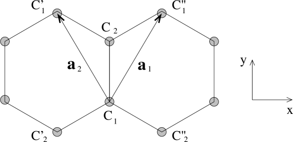
Figure 6: Two atoms, $C_{1}$ and $C_{2}$, in a graphene unit cell and basis vectors, ${\bf a}_{1}$ and ${\bf a}_{2}$.

Now let us consider the energy bands in carbon nanotube, which is formed by rolling up a graphene sheet. The circumference vector $\vec{C}_{N,M}=N\vec{a}_{1}+M\vec{a}_{2}$ uniquely defines the carbon nanotube. Periodic boundary condition around the CNT circumference leads to the quantization of the Bloch wave vector along that direction or the distinct band indices. For the armchair type $(n,n)$ tubes, $\vec{C}_{n,n}=n\sqrt{3}a~{}\hat{y}$ and the quantization rule is $k_{y}=2m\pi/n\sqrt{3}a$. The $(n,n)$ tubes repeat the unit cell (consisting of four atoms) $n$ times around the circumference, so that there should be $4n$ energy bands in the $(n,n)$ tubes. The band structure of $(n,n)$ nanotube is

$$E_{m\pm}^{(n)}(k) = \pm t\sqrt{1+4\cos\frac{m\pi}{n}\cos\frac{ka}{2}+4\cos^{2}\frac{ka}{2}},$$ (36)

where $m=0,1,\cdots,2n-1$. The relative phase difference between the wave functions of two atoms in a graphene unit cell can be written as

$$e^{i\delta} = \frac{1+2\exp[-i\frac{m\pi}{n}]\cos\frac{ka}{2}}{\sqrt{1+4\cos\frac{m\pi}{n}\cos\frac{ka}{2}+4\cos^{2}\frac{ka}{2}}}.$$ (37)

For the case of $m=0$ and $m=n$, the band structure as well as the phase difference are simplified.

$$E_{0\pm}(k) = \pm t~{}\left(1+2\cos\frac{ka}{2}\right),~{}\frac{c_{1}}{c_{2}}~{}=~{}\mp 1,$$ (38a)

$$E_{n\pm}(k) = \pm t~{}\left(1-2\cos\frac{ka}{2}\right),~{}\frac{c_{1}}{c_{2}}~{}=~{}\mp 1.$$ (38b)

Since we are interested in the spin polarized transport close to the Fermi level, we confine our interest to the $m=n$ bands.

Using the Bloch theorem, we can find the relative phase difference between two equivalent unit cells along the circumference in $(n,n)$ nanotubes, which is given by

$$|\psi^{\prime}\rangle = \exp[i\vec{k}\cdot(\vec{a}_{1}+\vec{a}_{2})]|\psi\rangle=\exp[i\frac{2\pi m}{n}]|\psi\rangle.$$ (39)

Especially for the $m=0,n$ bands, electron’s wave functions have a uniform phase from one unit cell to another around the CNT circumference. Combining all the relevant information, we summarize the $m=0,n$ bands and the relative phase in Fig. 7. The electronic states of the $\pi$ band ($c_{1}/c_{2}=1$) have uniform phase from one site to the next one in the edge layer. On the other hand, the $\pi^{*}$ band has an alternating phase, $\pm 1$, from one site to the next one along the circumference direction. This difference in phase will make the coupling strength between a CNT and the electrode depend on the symmetry states ($\pi$ or $\pi^{*}$) in a CNT.

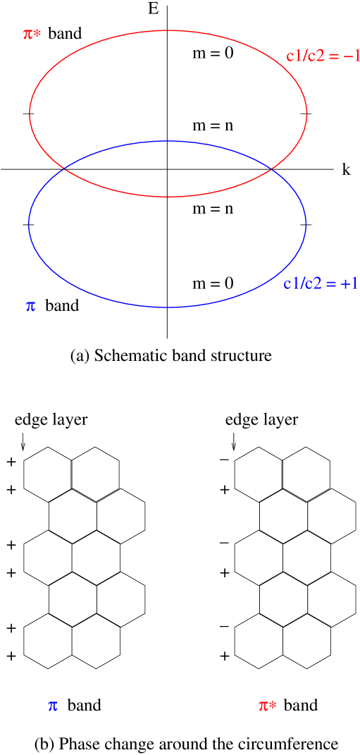
Figure 7: (Color online) (a) Schematic display of $\pi$ and $\pi^{*}$ bands. The lower ellipse represents the $\pi$ band, while the upper ellipse does the $\pi^{*}$ band. (b) Relative phase between two atoms in a graphene unit cell.

Appendix B Details about the coupling between CNT and FM electrodes

In this Appendix let us study the coupling matrix between the CNT and the electrode using the wave functions for free particles. We start with the wave functions for free particle in two-dimensional (2d) space. The obvious choice is the plane wave

$$\psi_{\vec{k}}(\vec{x}) = \langle\vec{x}|\vec{k}\rangle~{}=~{}\frac{e^{i\vec{k}\cdot\vec{x}}}{\sqrt{A}},~{}~{}~{}\epsilon=\frac{\hbar^{2}k^{2}}{2m}.$$ (40)

Here $A$ is the area of the two-dimensional system. The other one is the wave function with a cylindrical symmetry.

$$\psi_{km}(\vec{x}) = J_{m}(kr)e^{im\phi},~{}~{}~{}\epsilon=\frac{\hbar^{2}k^{2}}{2m}.$$ (41)

Here $J_{m}$ is the Bessel function. These two representations of wave function for free particle in 2d space satisfy the orthonormality relation

$$\int d^{2}x~{}\psi_{\vec{k}}^{*}(\vec{x})\psi_{\vec{k}^{\prime}}(\vec{x}) = \delta_{\vec{k},\vec{k}^{\prime}},$$ (42)

$$\int d^{2}x~{}\psi_{km}^{*}(\vec{x})\psi_{k^{\prime}m^{\prime}}(\vec{x}) = \delta_{m,m^{\prime}}\frac{2\pi}{k}\delta(k-k^{\prime}).$$ (43)

The following normalization is used for the cylindrical wave functions

$$\delta_{\epsilon,\epsilon^{\prime}} = \frac{1}{N_{2}(\epsilon)}~{}\delta(\epsilon-\epsilon^{\prime})~{}=~{}\frac{2\pi}{k}\delta(k-k^{\prime})\equiv\delta_{k,k^{\prime}}.$$ (44)

Here $N_{2}(\epsilon)$ is the density of states in 2d space and $\epsilon=\hbar^{2}k^{2}/2m$ and $\epsilon^{\prime}=\hbar^{2}k^{\prime 2}/2m$.

When the electrode is in contact with the armchair-type $(n,n)$ CNT, electrons in the electrode should belong to the same symmetry states as in the CNT if they have any chance to hop into the CNT. Since only the $\pi$ and $\pi^{*}$ states are responsible for the electron transport near the Fermi level under the neutral charge condition, we consider only the irreducible wave functions belonging to the $\pi$ and $\pi^{*}$ states. For the $(n,n)$ CNT,

$$\langle\phi|\pi m\rangle = \frac{1}{\sqrt{\pi}}\cos(nm\phi),$$ (45)

$$\langle\phi|\pi^{*}m\rangle = \frac{1}{\sqrt{\pi}}\sin(nm\phi).$$ (46)

Here $\phi$ is the azimuthal angle around the CNT axis. From these irreducible wave functions, we can deduce the following identities ($\bar{m}=-m$)

$$|\pi m> = \frac{1}{\sqrt{2}}(|nm\rangle+|n\bar{m}\rangle),$$ (47)

$$|\pi^{*}m> = \frac{i}{\sqrt{2}}(-|nm\rangle+|n\bar{m}\rangle).$$ (48)

Here $\langle\phi|m\rangle=e^{im\phi}/\sqrt{2\pi}$. For a free particle in 2d space, the wave functions for the $\pi$ and $\pi^{*}$ states are given by the following

$$\langle\vec{x}|\pi km\rangle = \sqrt{2}J_{nm}(kr)\cos(nm\phi),$$ (49)

$$\langle\vec{x}|\pi^{*}km\rangle = \sqrt{2}J_{nm}(kr)\sin(nm\phi).$$ (50)

In general, for a given $n$, the wave functions can be written down as

$$\langle\vec{x}|\pi km\rangle = R_{m}(kr)\cos(nm\phi),$$ (51)

$$\langle\vec{x}|\pi^{*}km\rangle = R_{m}(kr)\sin(nm\phi).$$ (52)

That is, the angular dependence is determined by the axial symmetry and does not change for any realistic wave functions. However, the radial part, reflecting the complexity of the system, will be more complicated than the Bessel function.

Let us consider the coupling between the $(n,n)$ CNT and the ferromagnetic electrode. Using the irreducible representations, the coupling Hamiltonian kimcox can be expanded as

$$H_{1} = \sum_{qkm}c_{\pi qkm}^{{\dagger}}\langle\pi qkm|V|j\rangle a_{j}+H.c.$$ (53)

$$+\sum_{qkm}c_{\pi^{*}qkm}^{{\dagger}}\langle\pi^{*}qkm|V|j\rangle a_{j}+H.c.$$

$$+\cdots.$$

The wave vector $\vec{K}=q\hat{z}+\vec{k}$ is defined in the electrode. $q$ is the wave number along the CNT axis and $\vec{k}$ is normal to the CNT axis. The omitted part (neither $\pi$ nor $\pi^{*}$ states) is not relevant to transport near the Fermi level, and will be neglected from our study. In the tight-binding Hamiltonian approach, we adopt the localized Wanier-type wave functions for the $p_{z}$ electrons at the carbon site. The coupling matrix can be written down as

$$\langle\pi qkm|V|j\rangle = V_{\pi m}(q,k)\cos(nm\phi_{j}),$$ (54)

$$\langle\pi^{*}qkm|V|j\rangle = V_{\pi^{*}m}(q,k)\sin(nm\phi_{j}).$$ (55)

Here $\phi_{j}$ represents the angular position of $j$-th carbon atom along the circumference at the edge layer of a $(n,n)$ CNT. In our study $V_{\pi m}(q,k)$ and $V_{\pi^{*}m}(q,k)$ are treated as phenomenological parameters. When the angle $\phi_{j}$ is substituted into the above coupling matrices, we get the desired simple forms

$$\langle\pi qkm|V|j\rangle = V_{\pi m}(q,k)\cos\frac{m\pi}{3},$$ (56)

$$\langle\pi^{*}qkm|V|j\rangle = (-1)^{j}V_{\pi^{*}m}(q,k)\sin\frac{m\pi}{3}.$$ (57)

The factors from angular functions are included in the coupling strength. As expected, the relative phase along the circumference of one layer correctly matches the $\pi$ and $\pi^{*}$ states in the CNT.

Appendix C Symmetry in coupling matrix elements between a carbon nanotube and ferromagnetic electrodes

Let us study the symmetry in the coupling matrix between the carbon nanotube and the ferromagnetic electrodes. Group theory tinkham is quite a powerful tool for the discussion about the symmetry in the coupling matrix elements. kimcox Since the armchair CNT has the discrete rotational symmetry about the carbon nanotube axis, the energy bands or levels can be classified according to the irreducible representations of the symmetry group of a CNT. Correspondingly the conduction electron states in the FM electrodes should have the same symmetry as the CNT states in order for electrons to be able to traverse the CNT.

As a concrete example, we consider the $(5,5)$ armchair-type CNT with a finite number of layers. Our discussion can be easily extended to the general $(n,n)$ armchair CNT. Depending on the even or odd layers, a finite CNT may have an additional symmetry along the nanotube axis. Since the symmetry in the coupling matrix is mainly determined by the rotational symmetry about the CNT axis, we are going to confine our discussion to this rotational symmetry.

The finite $(n,n)$ CNT belongs to $C_{nv}$ symmetry group. tinkham For the (5,5) CNT, there are four distinct classes: $E$ (identity), $2C_{5},2C_{5}^{2}$ (five-fold rotations) and $5\sigma_{v}$ (reflections). Correspondingly there are four irreducible representations for this group. The character table is summarized in Table 1 and can be used to find the irreducible representations for any reducible representation.

Table 1: Character table for $C_{5v}$ and decomposition of reducible representations. $a=2\cos 2\pi/5=(-1+\sqrt{5})/2$ and $b=2\cos 4\pi/5=(-1-\sqrt{5})/2$. $\gamma_{\pi}$: representation of $\pi$ orbitals. $\gamma_{m}$: representation of angular momentum states $m$ and $-m$.

$C_{5v}$	$E$	$2C_{5}$	$2C_{5}^{2}$	$5\sigma_{v}$
$A_{1}$	1	1	1	1
$A_{2}$	1	1	1	$-1$
$E_{1}$	2	a	b	0
$E_{2}$	2	b	a	0
$\gamma_{\pi}^{\phantom{{\dagger}}}$	20	0	0	0
$\gamma_{0}$	1	1	1	1
$\gamma_{m\neq 0}$	2	$2\cos\frac{2m\pi}{5}$	$2\cos\frac{4m\pi}{5}$	0

First we consider the electronic states in an infinite CNT. For the electronic structure, we adopt a single $\pi$ orbital approximation. In this case the $p_{z}$ orbital is located at each carbon site. Acting the symmetry operations on the CNT, we can find the characters of the $\pi$ orbitals. There are 20 carbon atoms for $(5,5)$ CNT in an extended unit cell around the circumference. Using the decomposition formula, we can readily find the number of irreducible representations.

$$\gamma_{\pi}^{\phantom{{\dagger}}} = 2A_{1}+2A_{2}+4E_{1}+4E_{2}.$$ (58)

There are four nondegenerate bands and eight bands with double degeneracy. When we take into account the phase variation of the $\pi$ and $\pi^{*}$ states along the circumference of the CNT, we can deduce that $\pi$ states belong to the $A_{1}$ irred. reps. On the other hand, the $\pi^{*}$ states belong to the $A_{2}$ irred. rep. Note that $\pi$ and $\pi^{*}$ states are invariant under discrete $C_{5}$ rotations. The $\pi$ states are invariant under $\sigma_{v}$, but the $\pi^{*}$ states change the sign under $\sigma_{v}$.

Now let us consider the angular momentum states about the CNT axis. The angular momentum operator $L_{z}$ is defined about the nanotube axis and its eigen states are well known to be $\psi_{m}(\phi)=e^{im\phi}$, with $L_{z}\psi_{m}(\phi)=m\psi_{m}(\phi)$. Since $\psi_{m}$ is the basis function for the continuous rotational symmetry, it cannot be the eigenstate for the discrete rotational symmetry, e.g., $C_{5v}$ for $(5,5)$ CNT. Acting the symmetry operations on these basis functions, we can find their character tables. The effect of the identity $E$, and the discrete rotations $C_{5},C_{5}^{2},C_{5}^{3},C_{5}^{4}$ on the angular momentum wave functions is obvious.

$$E\psi_{m}(\phi) = \psi_{m}(\phi),$$ (59a)

$${\cal R}_{\alpha}\psi_{m}(\phi) = \psi_{m}(\phi-\alpha)~{}=~{}e^{-im\alpha}\psi_{m}(\phi).$$ (59b)

The second operation ${\cal R}_{\alpha}$ is to rotate the wave function by the angle $\alpha$. The characters can be easily identified. For the operation of $\sigma_{v}$, a reflection, we have to find out its effect on the angular momentum operator $L_{z}$. The effect of $\sigma_{zx}$ (zx plane) and $\sigma_{zy}$ (zy plane)on $L_{z}$ is obvious.

$$\sigma_{zx}L_{z}\sigma_{zx}^{-1} = -L_{z},$$ (60a)

$$\sigma_{zy}L_{z}\sigma_{zy}^{-1} = -L_{z}.$$ (60b)

Note that $x\to x,y\to-y,z\to z$ and $p_{x}\to p_{x},p_{y}\to-p_{y},p_{z}\to p_{z}$ under $\sigma_{zx}$. Let us see if the above relation is true for an arbitrary reflection $\sigma_{v}$ where the $z$ axis lies on the reflection plane.

$$\sigma_{v}L_{z}\sigma_{v}^{-1} = -L_{z}?$$ (61)

We can prove this relation by the direct construction. Assume that the angle between the plane $\sigma_{v}$ and the plane $\sigma_{zx}$ is $\alpha$. Under $\sigma_{v}$, the coordinate $(x,y)$ transforms into a new one $(x^{\prime},y^{\prime})$. They are related by the equations

$$x^{\prime} = x\cos 2\alpha+y\sin 2\alpha,$$ (62a)

$$y^{\prime} = x\sin 2\alpha-y\cos 2\alpha.$$ (62b)

The linear momentum operators transform in the same way. Then we can readily show that $L_{z}=xp_{y}-yp_{x}$ transforms as

$$\sigma_{v}L_{z}\sigma_{v}^{-1} = -L_{z}.$$ (63)

Now let’s see the effect of $\sigma_{v}$ on the wave function $\psi_{m}(\phi)$. Intuitively $\sigma_{v}$ changes the direction of a rotation: right-hand rotation into left-hand rotation. Hence we can deduce that

$$\sigma_{v}\psi_{m}(\phi) = \psi_{m}(-\phi)~{}=~{}\psi_{-m}(\phi).$$ (64)

We can prove the above relation in a formal way using the transformation rule for $L_{z}$. Consider $\sigma_{v}L_{z}\psi_{m}(\phi)=m\sigma_{v}\psi_{m}(\phi)$. On the other hand, $\sigma_{v}L_{z}\psi_{m}(\phi)=\sigma_{v}L_{z}\sigma_{v}^{-1}\sigma_{v}\psi_{m}(\phi)=-L_{z}\sigma_{v}\psi_{m}(\phi)$. Since $L_{z}\sigma_{v}\psi_{m}(\phi)=-m\sigma_{v}\psi_{m}(\phi)$, we can deduce that

$$\sigma_{v}\psi_{m}(\phi) = c~{}\psi_{-m}(\phi).$$ (65)

Here $c$ is the $C$-number to be determined. Double operation of $\sigma_{v}$ is an identity so that $c^{2}=1$. We may choose $c=1$. Since $\sigma_{v}$ couples two states, $\phi_{m}$ and $\psi_{-m}$, we have to consider two states on the same footing. Let $\gamma_{m}$ denote the (reducible) representation in the functional space of $(\psi_{m},\psi_{-m})$. We can now build up the character tables for $\gamma_{m}$ considering the symmetry operations on the basis functions. For example,

$$\sigma_{v}\begin{pmatrix}\psi_{m}\cr\psi_{-m}\end{pmatrix} = \begin{pmatrix}0&1\cr 1&0\end{pmatrix}\begin{pmatrix}\psi_{m}\cr\psi_{-m}\end{pmatrix}.$$ (66)

Hence the character $\chi_{m}(\sigma_{v})=0$ (the trace of a transformation matrix). The other characters can be obtained using the same process and summarized in the Table 1. Using the decomposition rule, we can identify the irreducible representations.

$$\gamma_{0} = A_{1},$$ (67a)

$$\gamma_{5m} = A_{1}+A_{2},~{}m\neq 0,$$ (67b)

$$\gamma_{5m\pm 1} = E_{1},$$ (67c)

$$\gamma_{5m\pm 2} = E_{2}.$$ (67d)

From the above group theoretical analysis, we conclude that the $\pi$ states in a finite (5,5) CNT are coupled to the angular momentum states $\cos 5m\phi$, while the $\pi^{*}$ states are coupled to the states $\sin 5m\phi$. Other angular momentum states are coupled exclusively to the states belonging to the $E_{1}$ and $E_{2}$ irreducible representations, but never coupled to the $\pi$ and $\pi^{*}$ states.

References

- (1) I. Zutic, J. Fabian, and S. D. Sarma, Rev. Mod. Phys. 76, 323 (2004).
- (2) W. H. Butler, X.-G. Zhang, T. C. Schulthess, and J. M. MacLaren, Phys. Rev. B 63, 054416 (2001); J. Mathon and A. Umerski, Phys. Rev. B 63, 220403(R) (2001).
- (3) S. S. P. Parkin, C. Kaiser, A. Panchula, P. M. Rice, B. Hughes, M. Samant and S.-H. Yang, Nat. Mat. 3, 862 (2004); S. Yuasa, T. Nagahama, A. Fukushima, Y. Suzuki, and K. Ando, Nat. Mat. 3, 868 (2004).
- (4) J. M. De Teresa, A. Barthélémy, A. Fert, J. P. Contour, R. Lyonnet, F. Montaigne, P. Seneor, and A. Vaurès, Phys. Rev. Lett. 82, 4288 (1999); J. M. De Teresa, A. Barthélémy, A. Fert, J. P. Contour, F. Montaigne, and P. Seneor, Science 286, 507 (1999).
- (5) K. I. Lee, S. J. Joo, J. H. Lee, K. Rhie, T.-S. Kim, W. Y. Lee, K. H. Shin, B. C. Lee, P. LeClair, J.-S. Lee, and J.-H. Park, Phys. Rev. Lett. 98, 107202 (2007).
- (6) S. Yuasa, T. Nagahama, and Y. Suzuki, Science 297, 234 (2002).
- (7) S. Datta and B. Das, Appl. Phys. Lett. 56, 665 (1990).
- (8) K. Tsukagoshi, B. W. Alphenaar, and H. Ago, Nature (London) 401, 572 (1999).
- (9) J. R. Kim, H. M. So, J. J. Kim, and J. Kim, Phys. Rev. B 66, 233401 (2002).
- (10) A. Jensen, J. R. Hauptmann, J. Nygard, and P. E. Lindelof, Phys. Rev. B 72, 035419 (2005).
- (11) N. Tombros, S. J. van der Molen, and B. J. van Wees, Phys. Rev. B 73, 233403 (2006).
- (12) L. E. Hueso, J. M. Pruneda, V. Ferrari, G. Burnell, J. P. Valdés-Herrera, B. D. Simons, P. B. Littlewood, E. Artacho, A. Fert, and N. D. Mathur, Nature 445, 410 (2007).
- (13) R. Thamankar, S. Niyogi, B. Y. Yoo, Y. W. Rheem, N. V. Myung, R. C. Haddon, and R. K. Kawakami, Appl. Phys. Lett. 89, 033119 (2006).
- (14) S. Sahoo, T. Kontos, J. Furer, C. Hoffmann, M. Gräber, A. Cottet, and C. Schönenberger, Nature Phys. 1, 99 (2005).
- (15) H. T. Man, I. J. W. Wever, and A. F. Morpurgo, Phys. Rev. B 73, 241401(R) (2006).
- (16) N. Tombros, C. Jozsa, M. Popinciuc, H. T. Jonkman, and B. J. van Wees, Nature (London) 448, 571 (2007).
- (17) M. Nishioka and A. M. Goldmana, Appl. Phys. Lett. 90, 252505 (2007).
- (18) M. Ohishi, M. Shiraishi, R. Nouchi, T. Nozaki, T. Shinjo, and Y. Suzuki, J. J. Appl. Phys. 46, L605 (2007).
- (19) E. W. Hill, A. K. Geim, K. Novoselov, F. Schedin, and P. Blake, IEEE Trans. Mag. 42, 2694 (2006).
- (20) A. N. Pasupathy, R. C. Bialczak, J. Martinek, J. E. Grose, L. A. K. Donev, P. L. McEuen, and D. C. Ralph, Science 306, 86 (1999).
- (21) S. Sakaia, K. Yakushiji, S. Mitani, K. Takanashi, H. Naramoto, P. V. Avramov, K. Narumi, V. Lavrentiev, and Y. Maeda, Appl. Phys. Lett. 89, 113118 (2006).
- (22) E. Y. Tsymbal, A. Sokolov, I. F. Sabirianov, and B. Doudin, Phys. Rev. Lett. 90, 186602 (2003).
- (23) T.-S. Kim, C.-K. Lee, and B. C. Lee, J. Magn. Magn. Mater. 310, 1955 (2007).
- (24) X. Blase, L.X. Benedict, E.L. Shirley, and S.G. Louie, Phys. Rev. Lett. 72, 1878 (1994).
- (25) H. J. Choi, J. Ihm, Y.-G. Yoon, and S. G. Louie, Phys. Rev. B 60, R14009 (1999).
- (26) J. J. Palacios, A. J. Pérez-Jiménez, E. Louis, E. SanFabián, J. A. Vergés, Phys. Rev. Lett., 90, 106801 (2003).
- (27) L. P. Kadanoff and G. Baym, Quantum Statistical Mechanics (Benjamin, New York, 1962).
- (28) L.V. Keldysh, Zh. Éksp. Teor. Fiz. 47, 1515 (1964). [Sov. Phys. JETP 20, 1018 (1965)].
- (29) D.C. Langreth, 1976, in Linear and Nonlinear Electron Transport in Solids, Vol.17 of NATO Advanced Study Institute, Series B: Physicsi, edited by J.T. Devreese and V.E. van Doren (Plenum, New York, 1976), p. 3.
- (30) S. Hershfield, J. H. Davies, and J. W. Wilkins, Phys. Rev. Lett. 67, 3720 (1991).
- (31) Y. Meir and N. S. Wingreen, Phys. Rev. Lett. 68, 2512 (1992).
- (32) T.-S. Kim and S. Hershfield, Phys. Rev. B 63, 245326 (2001).
- (33) J. Taylor, H. Guo, J. Wang, Phys. Rev. B 63, 245407 (2001); Y. Liu, Phys. Rev. B 68, 193409 (2003); S. Ke, W. Yang, H. U. Baranger, J. Chem. Phys. 124, 181102 (2006).
- (34) D. Mann, A. Javey, J. Kong, Q. Wang, and N. H. Dai, Nano Lett. 3, 1541 (2003); A. Javey, J. Guo, Q. Wang, M. Lundstrom, and H. Dai, Nature (London) 424, 654 (2003).
- (35) N. Nemec, D. Tománek, and G. Cuniberti, Phys. Rev. Lett. 96, 076802 (2006).
- (36) M. P. Anantram, App. Phys. Lett. 78, 2055 (2001); M. P. Anantram, S. Datta, and Y. Xue, Phys. Rev. B 61, 14219 (2000).
- (37) J. Tersoff, D. R. Hamann, Phys. Rev. B 31, 805 (1985); G. I. Márk, L. P. Biró, and J. Gyulai, Phys. Rev. B 58, 12645 (1998);
- (38) T.-S. Kim and D. L. Cox, Phys. Rev. B 54, 6494 (1996).
- (39) T.-S. Kim, Phys. Rev. B 72, 024401 (2005).
- (40) S. Mukhopadhyay and I. Das, Phys. Rev. Lett. 96, 026601 (2006); Z.K. Keane, L.H. Yu, and D. Natelson, Appl. Phys. Lett. 88, 062514 (2006); K. I. Bolotin, F. Kuemmeth, A. N. Pasupathy, D. C. Ralph, Nano Lett. 6, 123 (2006).
- (41) S. Sanvito and A. R. Rocha, J. Comput. Theor. Nanosci. 3, 624 (2006).
- (42) W. J. M. Naber, S. Faez, and W. G. van der Wiel, J. Phys. D: Appl. Phys. 40, R205 (2007).
- (43) T.-S. Kim and S. Hershfield, Phys. Rev. B 67, 235330 (2003).
- (44) Z. A. Shao, W. Porod, and C. S. Lent, Phys. Rev. B 49, 7453 (1994).
- (45) T. Taniguchi and M. Büttiker, Phys. Rev. B 60, 13814 (1999).
- (46) R. Saito, M. Fujita, G. Dresselhaus, and M. S. Dresselhaus, Phys. Rev. B 46, 1804 (1992).
- (47) See, for example, M. Tinkham, Group theory and quantum mechanics (McGraw-Hill, New York).