Stimulating the production of deeply bound RbCs molecules with laser pulses:
the role of spin-orbit coupling in forming ultracold molecules

Abstract

We investigate the possibility of forming deeply bound ultracold RbCs molecules by a two-color photoassociation experiment. We compare the results with those for Rb₂ in order to understand the characteristic differences between heteronuclear and homonuclear molecules. The major differences arise from the different long-range potential for excited states. Ultracold ⁸⁵Rb and ¹³³Cs atoms colliding on the X ${}^{1}\Sigma^{+}$ potential curve are initially photoassociated to form excited RbCs molecules in the region below the Rb(5S) + Cs(6P_1/2) asymptote. We explore the nature of the $\Omega=0^{+}$ levels in this region, which have mixed A ${}^{1}\Sigma^{+}$ and b ${}^{3}\Pi$ character. We then study the quantum dynamics of RbCs by a time-dependent wavepacket (TDWP) approach. A wavepacket is formed by exciting a few vibronic levels and is allowed to propagate on the coupled electronic potential energy curves. We calculate the time-dependence of the overlap between the wavepacket and ground-state vibrational levels. For a detuning of 7.5 cm^-1 from the atomic line, the wavepacket for RbCs reaches the short-range region in about 13 ps, which is significantly faster than for the homonuclear Rb₂ system; this is mostly because of the absence of an $R^{-3}$ long-range tail in the excited-state potential curves for heteronuclear systems. We give a simple semiclassical formula that relates the time taken to the long-range potential parameters. For RbCs, in contrast to Rb₂, the excited-state wavepacket shows a substantial peak in singlet density near the inner turning point, and this produces a significant probability of deexcitation to form ground-state molecules bound by up to 1500 cm^-1. The short-range peak depends strongly on nonadiabatic coupling and is reduced if the strength of the spin-orbit coupling is increased. Our analysis of the role of spin-orbit coupling concerns the character of the mixed states in general and is important for both photoassociation and stimulated Raman deexcitation.

I Introduction

The study of cold molecules, below 1 K, and ultracold molecules, below 1 mK, offers many new opportunities for chemical and molecular physics. Cold molecules open up a new regime for molecular collisions in which classical physics breaks down completely and a quantal description is needed for all degrees of freedom. Collisions in this regime are dominated by long-range forces and exhibit resonance phenomena that can be controlled by applied electric and magnetic fields. Cold molecules also present new opportunities for precision measurement and open up possibilities for measuring quantities such as the dipole moment of the electron and the time-dependence of fundamental “constants”.

There is particular interest in ultracold polar molecules, because dipolar species interact more strongly and at much longer range than non-polar species. Dipolar quantum gases are predicted to exhibit new phenomena such as anisotropic Bose-Einstein condensation Leggett (2001) and may have applications in quantum information processing Rabl et al. (2006). They also provide opportunities for engineering highly correlated quantum phases Büchler et al. (2007).

Molecules can be formed in ultracold atomic gases by both magnetoassociation and photoassociation Jones et al. (2006); Hutson and Soldán (2006); Köhler et al. (2006), and there have been considerable advances in using such methods to produce heteronuclear alkali metal dimers Wang et al. (2004); Sage et al. (2005); Hudson et al. (2008); Kerman et al. (2004a, b); Haimberger et al. (2004); Kraft et al. (2006); Deiglmayr et al. (2008). However, both photo- and magnetoassociation initially produce molecules in very high vibrational levels, which are only very weakly dipolar even for heteronuclear species. There is therefore great interest in producing ultracold molecules in low-lying vibrational states. For example, Sage et al. Sage et al. (2005); Hudson et al. (2008) have succeeded in producing small numbers of ultracold RbCs molecules in the ground vibronic state by a four-photon photoassociation scheme using continuous-wave lasers, while Deiglmayr et al. Deiglmayr et al. (2008) have produced LiCs molecules with a two-photon scheme. Both these approaches include a spontaneous emission step, but Ni et al. Ni et al. (2008) have very recently produced KRb molecules in the lowest vibrational levels of the lowest singlet and triplet electronic states by magnetoassociation followed by a coherent two-photon process (stimulated Raman adiabatic passage, STIRAP). Danzl et al. Danzl et al. (2008a) have carried out analogous experiments on the homonuclear molecule Cs₂, while Lang et al. Lang et al. (2008) have produced Rb₂ molecules in the lowest level of the lowest triplet state.

Heteronuclear molecules differ from homonuclear molecules in several ways. The most important difference is that the excited-state potential curves correlating with ²S + ²P atoms have an $R^{-6}$ behavior at long range in the heteronuclear case but an $R^{-3}$ behavior in the homonuclear case, due to the resonant dipole interaction. Because of this, the Franck-Condon factors for photoassociation are quite different. In addition, the density of vibrational levels in the electronically excited state is different for $1/R^{6}$ and $1/R^{3}$ potentials.

Magnetoassociation must be carried out in tight traps at very low temperatures. However, there would be advantages in producing molecules in low-lying states at the somewhat higher temperatures (in the microkelvin regime) that are available in magnetooptical traps (MOTs), where the number of atoms available is often much larger. A very promising approach for this is photoassociation using shaped laser pulses. Short-lived molecules are formed in the excited electronic state by photoassociation using a short laser pulse (pump pulse) during the collision of two ultracold atoms. The excited molecules are then stabilized by stimulated emission using a second laser pulse (dump pulse) into the bound vibrational levels of the ground electronic state. Luc-Koenig et al. Luc-Koenig et al. (2004a, b) and Koch et al. Koch et al. (2006a, b) have simulated this process for homonuclear diatomic molecules such as Cs₂ and Rb₂, and initial experiments on these systems have been reported by Salzmann et al. Salzmann et al. (2006, 2008) and Brown et al. Brown et al. (2006). Similar experiments can be envisioned for heteronuclear molecules, with the use of evolutionary algorithms or other strategies to maximize the rate of production of ground-state molecules. However, a theoretical study of short-pulse photoassociation of heteronuclear molecules has not yet been carried out. In this paper, we consider RbCs as a prototype heteronuclear molecule and we study the possibility of forming ground-state RbCs molecules through pump-dump photoassociation.

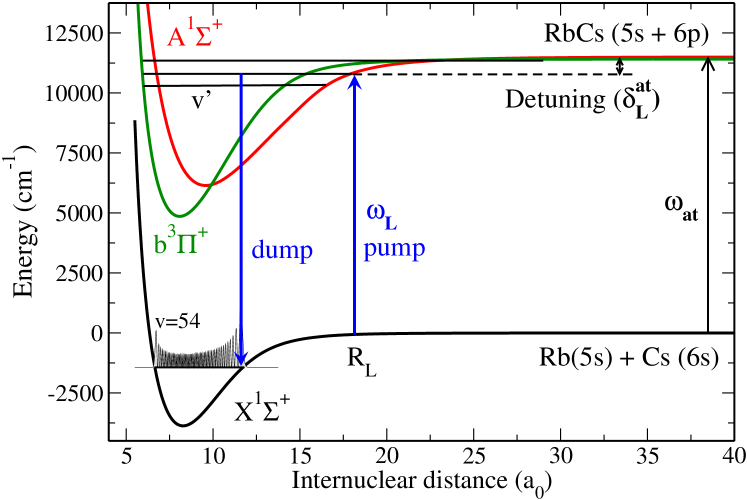
Figure 1: The potential curves and laser pulse scheme considered here. The potential curves correspond to the ground X ${}^{1}\Sigma^{+}$ and the excited A ${}^{1}\Sigma^{+}$ and b ${}^{3}\Pi$ states. A picosecond laser pulse is used to excite few vibronic levels in the excited state to form a wavepacket. A second laser pulse is used to dump the wavepacket to the ground X ${}^{1}\Sigma^{+}$ state after an appropriate time delay. The vibrational wavefunction of the target level of the dump pulse, $v=54$, is also displayed.

We consider the photoassociation of a colliding pair of ⁸⁵Rb and ¹³³Cs atoms, initially in their ground state. Absorption of a photon red-detuned from the atomic Rb(5S) + Cs(6P_1/2) asymptote forms an excited-state molecule around internuclear distance $R_{L}$, as shown in Fig. 1. When spin-orbit coupling is included there are 8 electronic states that correlate with the excited 5S_1/2 + 6P_1/2 and 5S_1/2 + 6P_3/2 asymptotes: two $0^{+}$ states, two $0^{-}$ states, three $\Omega=1$ states and one $\Omega=2$ state Kotochigova and Tiesinga (2005). These correlate at short range with the A ${}^{1}\Sigma^{+}$, b ${}^{3}\Pi$, B ${}^{1}\Pi$ and c ${}^{3}\Sigma^{+}$ electronic states in Hund’s case (a) labelling.

Absorption of a photon from the ground X ${}^{1}\Sigma^{+}$ ($0^{+}$) state can produce excited-state molecules in $0^{+}$ or 1 states, while absorption from the a ${}^{3}\Sigma^{+}$ state (with $0^{-}$ and 1 components) can produce $0^{+}$, $0^{-}$, 1 and 2 states. We focus here on the $0^{+}$ excited states, which may be formed by combining the A ${}^{1}\Sigma^{+}$ and b ${}^{3}\Pi$ states. The c ${}^{3}\Sigma^{+}$ state does not contribute because it has only $0^{-}$ and 1 components and the B ${}^{1}\Pi$ state does not contribute because it has only an $\Omega=1$ component. Rotational couplings that would connect states of different $\Omega$ are neglected. This 2-state approximation is analogous to the approach used for the $0_{u}^{+}$ states in Cs₂ and Rb₂ Kokoouline et al. (1999), for which the strongly mixed singlet-triplet character of the vibronic wavefunctions was found to produce enhanced formation of ground-state molecules with binding energies on the order of 10 cm^-1 Koch et al. (2006b); Pechkis et al. (2007).

The pump pulse produces a non-stationary state made up of long-range excited-state levels of mixed singlet and triplet character. The corresponding wavepacket propagates towards short range under the influence of the excited-state potentials. After a suitable time delay, when a sufficient amount of the wavepacket has reached the short-range region, a dump pulse is activated to transfer the molecules into vibrational levels of the X ${}^{1}\Sigma^{+}$ electronic ground state.

We simulate the entire pump-dump process using a time-dependent wavepacket (TDWP) approach. Our goal is to optimize the parameters of the pump and dump pulses to maximize the production of molecules in deeply-bound levels of the ground state. We find that a crucial factor is the magnitude of the spin-orbit coupling near the avoided crossing. If the spin-orbit coupling is sufficiently strong, then the levels that lie on the lower adiabatic curve, which correlates with 5S + 6P_1/2 at long range, have mainly triplet character at short range. Such levels have low intensities for deexcitation. We therefore form the excited-state wavepacket by selective photoassociation into vibronic levels of the A ${}^{1}\Sigma^{+}$- b ${}^{3}\Pi$ electronically excited states that are strongly mixed by nonadiabatic coupling and have enhanced singlet character at short range. We estimate the parameters required for the dump pulse and the time delay by analyzing the time-dependence of the overlap between the singlet part of the wavepacket and the vibrational levels of the ground electronic state.

We find an important difference between photoassociation for heteronuclear and homonuclear molecules. The excited states of heteronuclear molecules have a lower density of vibrational levels near dissociation than those of homonuclear molecules, because of the long-range $R^{-3}$ term in the excited-state potentials for homonuclear species. Because of this, the atoms of heteronuclear molecules produced at long range experience a significantly faster classical acceleration towards one another than homonuclear molecules created at the same binding energy. The time delay required between the pump and dump pulses is thus smaller in the heteronuclear case (about 13 ps for RbCs with a detuning of 7.5 cm^-1 from the atomic line) than in the homonuclear case. However, even for heteronuclear molecules, there is little probability of producing ground-state molecules within the duration of a single pulse of less than a few ps.

The paper is organized as follows. In section II, we discuss the potential energy curves and spin-orbit coupling functions used in this study. In sections III and IV we explore the dependence of the zero-energy $s$-wave scattering lengths on the interaction potentials and discuss their influence on the Franck-Condon factors for photoassociation. In section V we describe wavepacket studies of the photoassociation process and the subsequent formation of ground-state molecules. At each stage, the results for RbCs are compared with those for Rb₂ in order to establish the similarities and differences between heteronuclear and homonuclear molecules.

II Potential Curves

Several studies of the potential energy curves for RbCs have been published. Obtaining accurate potentials is not a straightforward task, because electronic structure calculations are very difficult for such heavy atoms. Experimental results are available for some states Fellows et al. (1999); Bergeman et al. (2003), but are sparse or nonexistent for others. Only some of the theoretical potentials include spin-orbit coupling effects; for example the relativistic curves of Kotochigova and Tiesinga Kotochigova and Tiesinga (2005) include avoided crossings which are absent in the older pseudopotential results of Allouche et al. Allouche et al. (2000).

The potential curves for the electronic states of RbCs considered here, neglecting spin-orbit coupling, are shown in Fig. 1. From the viewpoint of photoassociation, the most important parts of the curves are the long-range tails. In this study we have chosen for simplicity to use the ab initio results of Allouche et al. Allouche et al. (2000) at short range (bond lengths $R<15$ $a_{0}$). For the long-range potentials, in the ground state, we use the experimentally derived parameters of Fellows et al. Fellows et al. (1999), with C₆ replaced by the more recent value of Derevianko et al. Derevianko et al. (2001). These parameters are equivalent to column V of Table 2 in Ref. Jamieson et al., 2003. The Le Roy radius for the ground X ${}^{1}\Sigma^{+}$ state is 24.4 $a_{0}$, but a smooth match between the long-range and short-range potentials was best achieved at 16.5 $a_{0}$. For the excited singlet and triplet states, we use the theoretical long-range parameters of Marinescu and Sadeghpour Marinescu and Sadeghpour (1999), corresponding to the Rb(5S) + Cs(6P) asymptote. For the excited states the matching between long-range and short-range curves was achieved at 16.5 $a_{0}$ and 24 $a_{0}$ for the A and b states respectively.

Spin-orbit coupling between the A ${}^{1}\Sigma^{+}$ and b ${}^{3}\Pi$ states plays an important role. Following Marinescu and Dalgarno Marinescu and Dalgarno (1996) and Aubert-Frécon et al. Aubert-Frécon et al. (1998), the effect of the spin-orbit coupling for the $0^{+}$ states is included in terms of a 2$\times$2 electronic Hamiltonian matrix,

$$H^{\rm el}=\begin{pmatrix}V_{{\rm A}\,^{1}\Sigma^{+}}(R)&\sqrt{2}W_{\rm SO}^{\Sigma\Pi}(R)\\ \sqrt{2}W_{\rm SO}^{\Sigma\Pi}(R)&V_{{\rm b}\,^{3}\Pi}(R)-W_{\rm SO}^{\Pi\Pi}(R)\end{pmatrix},$$

(1)

where $V_{{\rm A}\,^{1}\Sigma^{+}}(R)$ and $V_{{\rm b}\,^{3}\Pi}(R)$ are the Born-Oppenheimer potentials neglecting spin-orbit coupling. The diagonal and off-diagonal spin-orbit coupling elements are denoted $W_{\rm SO}^{\Pi\Pi}(R)$ and $W_{\rm SO}^{\Sigma\Pi}(R)$ respectively and are functions of the internuclear separation $R$ as shown in Fig. 2. At long range,

$$W_{\rm SO}^{\Pi\Pi}(R\rightarrow\infty)=W_{\rm SO}^{\Sigma\Pi}(R\rightarrow\infty) = \frac{\Delta E_{\rm SO}^{\rm Cs}}{3},$$

where $\Delta E_{\rm SO}^{\rm Cs}$ is the spin-orbit splitting of the $P$ state of atomic Cs. Bergeman et al. Bergeman et al. (2004) give a non-zero matrix element connecting the $\Omega=0$ components of the b ${}^{3}\Pi$ and c ${}^{3}\Sigma^{+}$ states but this is appropriate only for the $0^{-}$ component and does not influence the $0^{+}$ states. We use the spin-orbit coupling functions obtained by Fellows and Bergeman Fellows and Bergeman (2007), which were obtained by fitting to results from Fourier-transform spectroscopy Bergeman et al. (2003). The diagonal and off-diagonal spin-orbit couplings show a significant dip from their asymptotic values near the crossing between the A ${}^{1}\Sigma^{+}$ and b ${}^{3}\Pi$ potential energy curves. The two adiabatic potentials obtained by diagonalizing the electronic Hamiltonian of Eq. (1) are shown as an insert in Fig. 2.

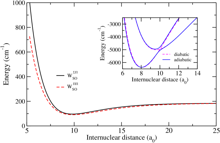
Figure 2: The diagonal and off-diagonal components $W^{\Pi\Pi}_{\rm SO}(R)$ and $W^{\Sigma\Pi}_{\rm SO}(R)$ of the spin-orbit coupling as a function of $R$. The avoided crossing between the two adiabatic potentials is shown in the inset.

For Rb₂ the potentials are more accurately known. In the present work, the ground-state X ${}^{1}\Sigma_{g}^{+}$ potential is obtained by combining the short-range results of Seto et al. Seto et al. (2000) with the long-range coefficients of Marte et al. Marte et al. (2002). The excited-state potentials are taken from Bergeman et al. Bergeman et al. (2006), who obtained potential curves and spin-orbit coupling functions for the A ${}^{1}\Sigma_{u}^{+}$ and b ${}^{3}\Pi_{u}$ states by combining photoassociation spectroscopy with short-range ab initio results Edvardsson et al. (2003). The corresponding curves for Rb₂ (not shown here) are qualitatively similar to those for RbCs, except for the important difference in long-range behavior.

Figure 3: RbCs s-wave scattering length for the X ${}^{1}\Sigma^{+}$ state, as a function of a scaling factor used to multiply the potential.

III Scattering length

A crucial parameter affecting low-energy scattering properties and the positions of high-lying excited states is the s-wave scattering length $a$. Calculations by Jamieson et al. Jamieson et al. (2003) produced values for $a$ ranging from 380 to 1 $a_{0}$ for the X ${}^{1}\Sigma^{+}$ state of RbCs, depending on the subtleties of the potential parameters. There are further uncertainties due to the choice of hyperfine states involved. In addition, even if the potential is known accurately, there is the possibility of controlling the scattering length with applied fields. We therefore investigate the dependence of photoassociation on the scattering lengths for both the ground and excited states.

Scattering lengths were calculated by solving the Schrödinger equation for zero-energy s-wave scattering numerically using Numerov integration. The long-range wavefunction was matched to Bessel and Neumann functions of fractional order Gribakin and Flambaum (1993) to take account of the long-range $R^{-n}$ potential and avoid the need to propagate to excessively large distances. We adjusted the scattering length by scaling the whole potential curve by a constant factor. As is well known, the scattering length is extremely sensitive to such scaling and passes through a pole whenever there is a bound state at exactly zero energy. For ⁸⁵Rb¹³³Cs a complete cycle is achieved within a scaling of just over 1%, as can been seen from Fig. 3. Rb₂ shows similar behavior.

Figure 4: Upper panel: Average bond length $\langle R\rangle$ for vibrational levels of RbCs in its A ${}^{1}\Sigma^{+}$ state as a function of the binding energy. Lower panel: Franck-Condon factors for photoassociation (in arbitrary units), calculated for a ground-state scattering length $a=66.3$ $a_{0}$. Note that the largest factors are off the top of the scale in this figure.

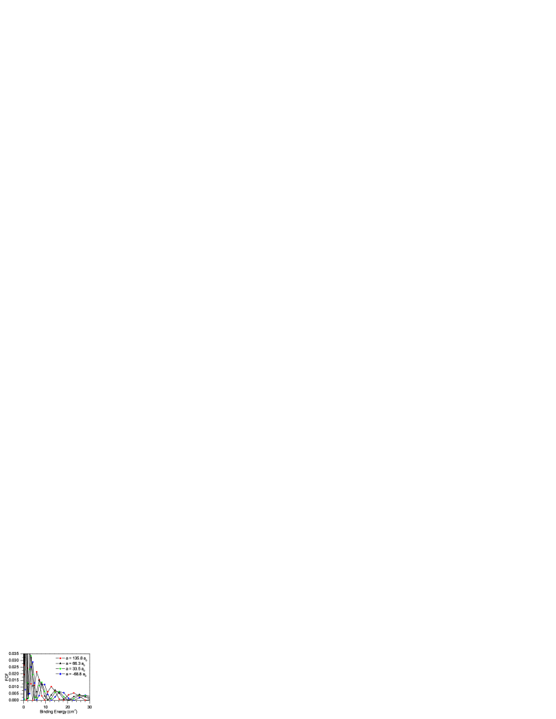
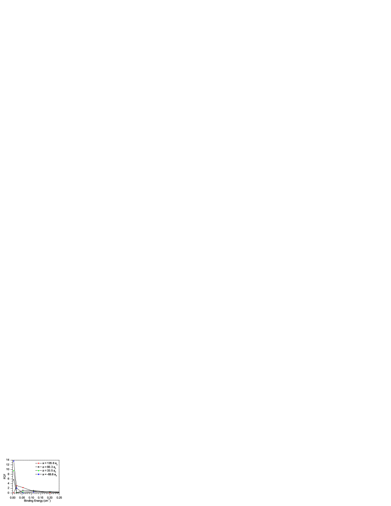
Figure 5: Franck-Condon factors for RbCs photoassociation, calculated for a variety of ground-state scattering lengths. The scale is arbitrary but is consistent between graphs.

IV Franck-Condon factors and their dependence on scattering lengths

We first calculate the Franck-Condon factors (FCFs) of relevance to photoassociation experiments for ⁸⁵Rb¹³³Cs and compare the results with those for the homonuclear ⁸⁵Rb₂ system. The purpose of this Section is to understand the qualitative differences between RbCs and Rb₂, which stem from the different long-range tails of the excited-state potential (proportional to $R^{-6}$ for RbCs and $R^{-3}$ for Rb₂). These qualitative differences are most simply illustrated using calculations that neglect the coupling between the A ${}^{1}\Sigma^{+}$ and b ${}^{3}\Pi$ states, and that is the approach we use in this Section. However, coupled calculations of FCFs have been carried out by Luc-Koenig Luc-Koenig (2008), and indeed the calculations described in Section V.3 to V.5 below use fully coupled wavefunctions.

The FCFs for photoassociation are calculated as the squares of overlap integrals between bound vibrational states in the excited A ${}^{1}\Sigma^{+}$ electronic potential and a low-energy scattering wavefunction on the ground-state potential. Both the bound and scattering states were obtained by Cooley-Numerov propagation Cooley (1961) for rotational angular momentum $N=0$. A LeRoy-Bernstein analysis Le Roy and Bernstein (1970) confirmed that every bound state had been found. The s-wave scattering function was calculated at a collision energy of 1 mK and normalized by setting its maximum amplitude to 1 as $R\rightarrow\infty$. The ground-state potential does not die off to 1 mK until $R\sim 110\ a_{0}$, so that the relative values of the resulting Franck-Condon factors should be valid for excitation to states dominated by distances $R<100\ a_{0}$.

Figure 4 shows the calculated FCFs for RbCs with $a=+66.3$ $a_{0}$ as a function of binding energy (detuning from the Cs atomic line), and the corresponding values of $\langle R\rangle$ for the excited vibrational states. The FCFs show a typical oscillating pattern as the bound and continuum states come into and out of phase with one another. For RbCs each peak of the envelope encompasses around 4 vibrational levels of the excited state. The most intense peak is just below the dissociation threshold, and the state at the center of this peak has $\langle R\rangle\approx$ 71 $a_{0}$. The next peaks in order of decreasing intensity correspond to $\langle R\rangle\approx$ 47, 37, 32, 29 and 26 $a_{0}$. The largest FCF occurs for the least-bound state, with $\langle R\rangle=150$ $a_{0}$, which is not part of an envelope. However, this state is bound by only 0.0007 cm^-1, and it is likely that frequencies this close to the atomic line would be blocked in an actual experiment.

Figure 6: Upper panel: Average bond length $\langle R\rangle$ for vibrational levels of Rb₂ in its A ${}^{1}\Sigma^{+}_{u}$ state as a function of the binding energy. Lower panel: Franck-Condon factors for photoassociation. The scale is arbitrary but is consistent with that for RbCs in Figs. 4 and 5. Note that the largest factors are off the top of the scale in this figure.

To investigate the effect of adjusting the ground-state scattering length, we have repeated the Franck-Condon calculations for $a=135.8$, 33.5, and $-68.8$ $a_{0}$, corresponding to potential scaling factors of 0.9965, 1.0015 and 1.0039 respectively. The results are shown in Fig. 5. It may be seen that changing the scattering length shifts the positions of the peaks in the envelope of the intensity distribution. Nevertheless, the peak intensities themselves follow a curve that is only very weakly potential-dependent. The peak intensities are thus almost a single-valued function of binding energy.

Scaling the potential curve for the excited state, while keeping the ground-state scattering length constant, shifts the positions of the individual lines but does not alter the positions of the peaks in the intensity distribution. This effect is shown for $a=+66.3$ $a_{0}$ in Fig. 8: the frequencies that correspond to vibrational levels shift as the potential is scaled, but the envelope of the FCFs does not change. Since a laser pulse will always cover a range of binding energies, it is this envelope that matters more than the specific position of the levels and the overall transition probabilities will not be greatly affected by changes in the excited-state scattering length.

The Franck-Condon factors for photoassociation to form Rb₂ are shown in Fig. 6. The potential curve used here has $a=157.9$ $a_{0}$. Once again the FCFs show an oscillatory structure. The major difference from RbCs is that the oscillations in the envelope of line intensities are slower as a function of binding energy and the lines themselves are much more densely packed because of the greater density of states for an $R^{-3}$ potential. The overall values of the FCFs are also somewhat larger in the homonuclear case.

Figure 7: Franck-Condon factors for different values of the ground-state scattering length, shown on a log-log plot for RbCs (upper panel) and Rb₂ (lower panel). Note that the peak values lie on a straight line in each case, but with a different slope, corresponding to a different power-law dependence on binding energy.

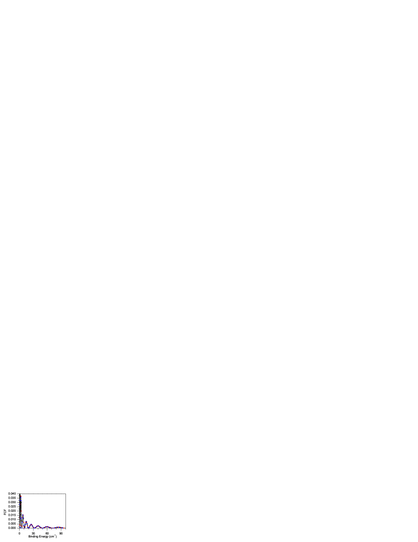
Figure 8: Franck-Condon factors for different scalings of the upper potential with the unscaled ground-state potential. Black, blue and red symbols are for scalings of 1.0, 1.001 and 1.005 respectively.

Another significant difference between the heteronuclear and homonuclear cases is shown in Fig. 7. On a log-log plot, the intensities of the peak envelopes vary almost linearly with binding energy $E_{\rm D}-E_{v}$ near dissociation. This corresponds to a power-law dependence on binding energy. However, the powers involved are clearly different for the two cases: about $(E_{\rm D}-E_{v})^{-1}$ for the homonuclear case and $(E_{\rm D}-E_{v})^{-1.6}$ for the heteronuclear case. This will be significant in designing pulsed-laser experiments, because the intensity will fall off considerably faster with detuning (from the atomic line) in the homonuclear case than in the heteronuclear case. Thus a broad pulse will excite a wavepacket in which the relative population of deeper levels is lower in the heteronuclear case.

V Time-dependent calculations

V.1 Vibrational periods

In section V.2 we study the photoassociation process in a time-dependent wavepacket approach. However, we can make a rough estimate of the time needed for the wavepacket to evolve from long to short range by considering the vibrational half-period,

$$t_{1/2}=\frac{1}{2\nu}=\frac{h}{2\left(\frac{dE_{v}}{dv}\right)},$$ (2)

where $\nu$ is the classical vibrational frequency. The vibrational spacing $dE_{v}/dv$ may be calculated exactly for a particular potential curve but it is instructive to consider its value in long-range theory. If only the leading term in the long-range potential is included, $V(R)=-C_{n}R^{-n}$, the vibrational period may be written semiclassically Le Roy (1973)

$$\frac{dE_{v}}{dv}=K_{n}(E_{\rm D}-E_{v})^{(n+2)/2n},$$ (3)

where

$$K_{n}=\frac{\overline{K}_{n}}{\mu^{1/2}C_{n}^{1/n}}=\frac{(2\pi)^{1/2}h}{\mu^{1/2}C_{n}^{1/n}}\left(\frac{n\Gamma(1+1/n)}{\Gamma(1/2+1/n)}\right),$$ (4)

$\mu$ is the reduced mass and $\Gamma$ is the gamma function. Le Roy has tabulated numerical values of the coefficients $\overline{K}_{n}$ Le Roy (1973). The times obtained for wavepackets corresponding to each of the main peaks in Fig. 4 are given in Table 1 for ⁸⁵Rb¹³³Cs. The half-periods vary from over 100 ps at small detunings to under 1 ps for a detuning of $-315$ cm^-1. Although the positions of the individual maxima are sensitive to details of the potential, the time taken is an almost single-valued function of the binding energy (laser detuning) for a particular long-range potential and reduced mass.

Table 1: Vibrational half-periods for an RbCs molecule at energies corresponding to maxima in the intensity distribution for photoassociation. The index $m$ labels the successive maxima, starting at the dissociation limit.

$m$	binding energy	$\langle R\rangle$	relative	$t_{1/2}$
	(cm-1)	($a_{0}$)	intensity	(ps)
$1$	$-0.0063$	71	$\sim 1.5$	290
$2$	$-0.76$	47	0.13	54
$3$	$-2.9$	37	0.038	22
$4$	$-7.3$	32	0.016	12
$5$	$-15$	29	0.0080	7.5
$6$	$-26$	26	0.0045	5.2
$7$	$-41$	24	0.0027	3.8
$8$	$-57$	23	0.0018	3.0
$9$	$-82$	20	0.0013	2.4
$10$	$-113$	20	0.00096	1.93
$11$	$-150$	19	0.00073	1.56
$12$	$-194$	18	0.00056	1.26
$13$	$-245$	17	0.00041	1.13
$14$	$-315$	17	0.00028	0.97

The times taken for RbCs are significantly shorter than those for Rb₂, shown in Table 2. For example, for a detuning of 25 cm^-1 from the atomic line, the classical time is about 13 ps for Rb₂ but 5 ps for RbCs.

The classical model used here is of course considerably oversimplified and neglects features such as the spreading of a wavepacket as it propagates inwards. A full treatment of the time evolution requires quantum-mechanical calculations as described below.

Table 2: Vibrational half-periods for an Rb₂ molecule at energies corresponding to maxima in the intensity distribution for photoassociation. The index $m$ labels the successive maxima, starting at the dissociation limit.

$m$	binding energy	$\langle R\rangle$	relative	$t_{1/2}$
	(cm-1)	($a_{0}$)	intensity	(ps)
$1$	$-0.017$	500	12	6300
$2$	$-0.038$	380	8.5	3200
$3$	$-0.10$	270	5.2	1400
$4$	$-0.49$	160	2.4	380
$5$	$-5.1$	75	0.36	54
$6$	$-27$	43	0.043	13
$7$	$-56$	34	0.014	7.3
$8$	$-91$	29	0.007	4.9
$9$	$-135$	26	0.004	3.5

V.2 Wavepacket model and methods

In the time-dependent wavepacket approach, the photoassociation reaction starts with two cold atoms in the ground electronic state with relative kinetic energy $E_{\rm kin}$. Absorption of a photon red-detuned by an energy $\hbar\omega_{L}$ from the atomic resonance line at $\hbar\omega_{\rm at}$ produces a molecule in the excited electronic state as shown in Fig. 1. The Hamiltonian describing optical transitions between the X ${}^{1}\Sigma^{+}$ electronic ground state and the coupled A ${}^{1}\Sigma^{+}$ and b ${}^{3}\Pi$ excited states can be represented in the diabatic basis as

$$\bm{\mathsf{\hat{H}}}=\left(\begin{array}[]{ccc}\bm{\mathsf{\hat{T}}}+V_{{\rm X}^{1}\Sigma^{+}}(R)&\bm{\mu}(R)\cdot\bm{E}(t)&0\\ \bm{\mu}(R)\cdot\bm{E}(t)&\bm{\mathsf{\hat{T}}}+V_{{\rm A}^{1}\Sigma^{+}}(R)-\hbar\omega_{L}&\sqrt{2}W^{\Sigma\Pi}_{\rm SO}(R)\\ 0&\sqrt{2}W^{\Sigma\Pi}_{\rm SO}(R)&\bm{\mathsf{\hat{T}}}+V_{{\rm b}^{3}\Pi}(R)-W^{\Pi\Pi}_{\rm SO}(R)-\hbar\omega_{L}\end{array}\right)\,,$$ (8)

where $\bm{\mathsf{\hat{T}}}$ is the kinetic energy operator and $V_{i}(R)$ are the respective potential energy curves. Assuming the dipole and rotating-wave approximations, the coupling between the X ${}^{1}\Sigma^{+}$ and A ${}^{1}\Sigma^{+}$ electronic states is represented by the scalar product between the transition dipole moment, $\bm{\mu}(R)$, and the polarization vector of the laser field, $\bm{E}(t)$. In the present work the $R$-dependence of $\bm{\mu}(R)$ is neglected and it is represented by its asymptotic value. The A ${}^{1}\Sigma^{+}$ and b ${}^{3}\Pi$ excited states are coupled by the spin-orbit interaction. The hyperfine interaction can be neglected because the associated timescale is much longer than the femtosecond or picosecond laser pulses, so that the hyperfine interaction is not resolved for the processes considered in the present study.

The Hamiltonian, Eq. (8), is represented on a Fourier grid with a variable grid step Kokoouline et al. (1999). Details of the mapped Fourier Grid Hamiltonian (FGH) method are described in refs. Willner et al., 2004 and Kallush and Kosloff, 2006. Using the FGH method, we are able to extend the spatial grid to $R\sim 10^{3}\ a_{0}$ using only 1023 grid points; this is sufficient both to represent the bound vibronic levels and to approximate the scattering continuum in the ultracold temperature regime by box states Koch et al. (2006c).

To describe the short-pulse photoassociation process, we solve the time-dependent Schrödinger equation (TDSE),

$$i\hbar\frac{\partial}{\partial t}\Psi(t)=\bm{\mathsf{\hat{H}}}(t)\Psi(t),$$ (9)

by expanding the evolution operator $\exp[-i\bm{\mathsf{\hat{H}}}t/\hbar]$ in terms of Chebychev polynomials Kosloff (1994). Because of the large extent of the grid and the very small kinetic energy of the system, it is not necessary to enforce an absorbing boundary condition at the edge of the grid.

V.3 Analysis of the coupled vibronic wavefunctions

Diagonalization of the Hamiltonian of Eq. (8) with $\bm{E}(t)$ set to zero yields the binding energies and vibronic wavefunctions and allows the calculation of FCFs, rotational constants, etc. For RbCs it produces 136 bound vibronic levels for the X ${}^{1}\Sigma^{1}$ ground electronic state and 398 levels for the coupled A ${}^{1}\Sigma^{+}$ and b ${}^{3}\Pi$ electronic states. The eigenfunctions of the excited electronic states are perturbed by the spin-orbit coupling and have mixed singlet and triplet character. The highest excited-state level has a binding energy of 0.002 cm^-1, which differs slightly from the result in Section IV because the latter neglected the coupling between the singlet and triplet states.

When two electronic states interact and their curves cross, there are two quite different limiting cases that may be considered to be “uncoupled”. If the coupling near the crossing point is very weak (compared to the local vibrational spacings), the crossing is only weakly avoided and the eigenstates of the coupled system are close to those of the individual diabatic (crossing) electronic states. Conversely, if the coupling is strong, the crossing is strongly avoided and the best zeroth-order picture is to consider eigenfunctions of the adiabatic states, defined by the non-crossing upper and lower adiabatic curves. In this case the adiabatic states themselves change character from one side of the crossing to the other, so that in the present case the zeroth-order states are predominantly singlet on one side of the crossing and predominantly triplet on the other. The couplings between the adiabatic states are provided by nonadiabatic couplings (which are related to off-diagonal matrix elements of $d/dR$ and $d^{2}/dR^{2}$).

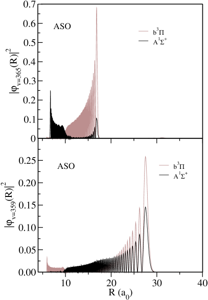
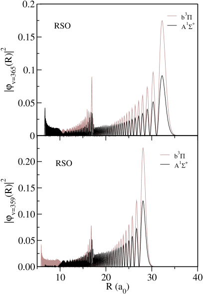
Figure 9: Eigenfunctions of the coupled excited-state potentials corresponding to $v=359$ and 365. Left-hand panels: results obtained with constant asymptotic spin-orbit coupling (ASO). Right-hand panels: results obtained with $R$-dependent spin-orbit coupling (RSO).

The wavefunction for a mixed vibronic state may be written

$$\varphi_{1}^{v}(R)\psi_{1}+\varphi_{3}^{v}(R)\psi_{3}$$ (10)

where the functions $\varphi_{1}^{v}(R)$ and $\varphi_{3}^{v}(R)$ are vibrational wavefunctions and $\psi_{1}$ and $\psi_{3}$ are electronic functions for the singlet and triplet excited states respectively. It is useful to compare the eigenstates that are obtained for two different cases, as shown in Fig. 9. The two panels on the left show RbCs eigenstates calculated with the spin-orbit coupling functions fixed at their asymptotic value, $\Delta E_{\rm SO}^{\rm Cs}=554.04$ cm^-1 (corresponding to $W_{\rm SO}^{\Sigma\Pi}=184.68$ cm^-1, which is considerably larger than the experimentally derived value Fellows and Bergeman (2007) around the crossing point of the diabatic curves ($W_{\rm SO}^{\Sigma\Pi}\approx 100$ cm^-1, see Fig. 2). These will be referred to as ASO (asymptotic spin-orbit) calculations. The two levels shown are for vibrational indices $v^{\prime}=359$, with binding energy 22.19 cm^-1, and $v^{\prime}=365$, with binding energy 10.01 cm^-1. It may be seen that for both ASO wavefunctions there is a switchover from singlet to triplet character around the avoided crossing ($R\sim 10\ a_{0}$), but in opposite directions. This occurs because the states are nearly adiabatic: the function for $v^{\prime}=365$ lies on the upper adiabatic curve, so has mainly singlet character inside the crossing and mainly triplet character outside. The function for $v^{\prime}=359$ lies on the lower adiabatic curve, so that it has mostly triplet character at short range. Outside the crossing, it has mainly singlet character in the region where the singlet and triplet curves are separated by more than the spin-orbit coupling. At long range ($R>{\sim 20}\ a_{0}$), however, it reacquires the triplet admixture characteristic of an $\Omega=0$ state at the 5S + 6P_1/2 threshold, yielding a 2:1 ratio of triplet to singlet probability. It stretches to considerably greater internuclear distance because of the different turning points for the two adiabatic states.

The near-adiabatic vibronic levels obtained for the ASO case provide a context to understand the eigenstates obtained with the $R$-dependent spin-orbit (RSO) coupling function, shown in the panels on the right of Fig. 9. In the RSO case the levels with index numbers $v^{\prime}=359$ and 365 have binding energies 17.79 cm^-1 and 7.53 cm^-1, respectively. The $v^{\prime}=359$ level exists mostly on the lower adiabatic curve, and has triplet character with only a small singlet admixture at short range and switches over to singlet character (with the same characteristic triplet admixture as before) outside $R=10\ a_{0}$. Nevertheless, there is significant nonadiabatic mixing which introduces upper-state character, shown by the peaks in probability densities around the outer turning point of the upper curve near $R\sim 17\ a_{0}$. The $v^{\prime}=365$ level is more strongly mixed, with a larger contribution from the upper adiabatic state that makes it predominantly singlet at short range. However, this state too has substantial lower-state character so that it does have density out to the outermost turning point ($R\sim 33\ a_{0}$ in this case). It is notable that both RSO eigenstates have significantly enhanced singlet density near the outer turning point of the upper curve ($R\sim 17\ a_{0})$. This is the feature that in Rb₂ was responsible for enhanced deexcitation to levels of the ground state bound by up to 10 cm^-1 Koch et al. (2006b); Pechkis et al. (2007). However, the wavefunction for $v^{\prime}=365$ also has substantial singlet density near the inner turning point of the singlet state; this is a feature that was not observed for Rb₂ (see Fig. 2 of ref. Koch et al., 2006b), and as will be seen below it allows deexcitation to even more deeply bound levels. The fact that the wavefunction can have significant singlet density both at this turning point and at the outermost turning point arises from nonadiabatic coupling between the upper and lower adiabatic states.

In an alternative approach, the nonadiabatic mixings could be shown in an adiabatic representation, displaying the components of the vibrational wavefunctions on the two $0_{u}^{+}$ states. This would emphasize the nearly adiabatic character of the ASO wavefunctions but would hide their switchover from singlet to triplet character near the avoided crossing.

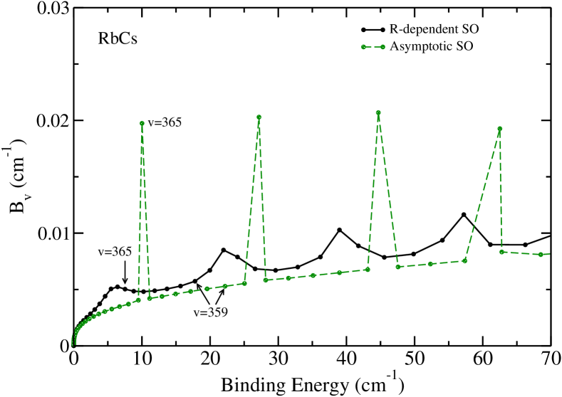
Figure 10: Rotational constants $B_{v}^{\prime}=\langle h/(8\pi^{2}c\mu R^{2})\rangle$ corresponding to the vibronic levels of the coupled A ${}^{1}\Sigma^{+}+b^{3}\Pi$ excited electronic states for RbCs.

The character of the mixed levels, as a function of vibrational quantum number, may be seen very clearly in the calculated rotational constants for the coupled levels ($B_{v}=\langle h/(8\pi^{2}c\mu R^{2})\rangle$), which are shown in Fig. 10 for both the ASO and RSO cases. In the ASO case, the rotational constants form two almost independent series, with the higher values corresponding to levels that are predominantly on the upper adiabatic curve. The upper state has a larger vibrational spacing than the lower state. In the RSO case, the peaks in rotational constants correspond to levels with a significant contribution from the upper adiabatic state. However, it may be seen that in this case the nonadiabatic coupling is strong enough to spread the character of each upper-curve vibronic state across several eigenfunctions of the coupled problem, so that the peaks are not very large. There are no eigenstates of the coupled problem that are predominantly on the upper adiabatic curve.

The rotational constants for RbCs may be compared with those for Rb₂ Kokoouline et al. (1999); Bergeman et al. (2006), shown in Fig. 11. Rb₂ exhibits nonadiabatic mixing that is intermediate between the ASO and RSO cases for RbCs. For Rb₂ the extent of the mixing has been shown to be isotope-dependent Fioretti et al. (2007).

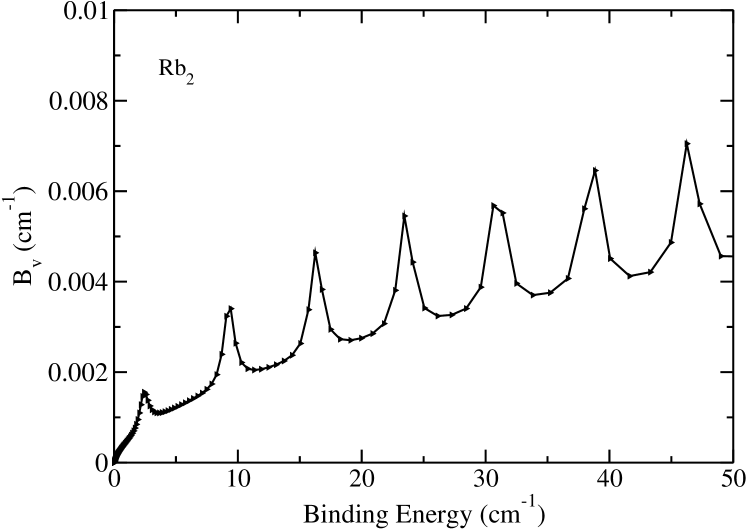
Figure 11: Rotational constants $B_{v}^{\prime}=\langle h/(8\pi^{2}c\mu R^{2})\rangle$ corresponding to the vibronic levels of the coupled A ${}^{1}\Sigma^{+}+b^{3}\Pi$ excited electronic states of Rb₂.

The existence of bound states with singlet character both at long range and near the inner turning point will also be important in designing fixed-frequency schemes to populate deeply-bound ground-state levels by STIRAP and related methods. Such schemes will be most efficient when they proceed via mixed levels with population on both the upper and lower adiabatic curves.

V.4 Photoassociation with a short laser pulse

The pump-dump scheme considered here is shown schematically in Fig. 12. Each laser pulse is assumed to be transform-limited,

$$E(t)=E_{0}f(t)\cos(\omega_{L}t),$$ (11)

with a Gaussian profile $f(t)=\exp-\alpha(t-t{\rm c})^{2}$. The pulse has central frequency $\omega_{L}/(2\pi)$ and maximum field amplitude $E_{0}$. The full width at half maximum (FWHM) of the intensity profile $E_{0}^{2}f(t)^{2}$ is $\tau_{L}=(2\ln 2/\alpha)^{-1/2}$. The corresponding FWHM frequency width is $\delta_{\omega}/(2\pi)=2\ln 2/(\pi\tau_{L})$. The Gaussian envelopes are centered at times $t=t_{\rm p}$ and $t_{\rm d}$ for the pump and dump pulses respectively.

Table 3: The parameters for the pump and dump pulse: detuning $\delta_{L}^{\rm at}$ from the atomic line, intensity $I_{L}$, temporal width $\tau_{L}$, spectral bandwidth $\delta_{\omega}$, and integrated pulse energy per area.

pulse	$\delta_{L}^{\rm at}$	$I_{L}$	$\tau_{L}$	$\delta_{\omega}/(2\pi c)$	Energy/Area
	(cm-1)	(W cm-2)	(ps)	(cm-1)	(J m-2)
pump (ASO)	$-10.01$	16.86	5.00	2.94	0.095
pump (RSO)	$-7.53$	16.86	5.00	2.94	0.095
dump (RSO)	1427.61	98.32	1.00	14.72	0.474

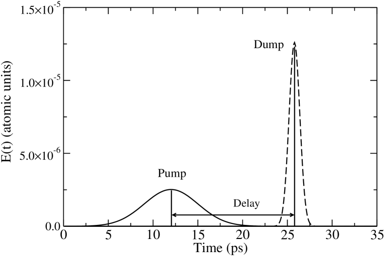
Figure 12: Schematic diagram of the laser pulse sequence considered in the present study. The pump and dump pulses are centered at 12.0 ps and 25.8 ps, respectively, with a time delay of 13.8 ps (note that $1\times 10^{-5}$ atomic units of electric field correspond to 5.14 MV/m).

The parameters used for the laser pulses in this study are given in Table 3. We choose the parameters of the pump pulse to excite a few excited-state vibronic levels $v^{\prime}$ close to the maxima in Fig. 10 where nonadiabatic coupling is strongest. The central frequency is chosen to be resonant with the level $v^{\prime}=365$, with a laser detuning from the atomic line $\delta_{L}^{\rm at}=7.53$ cm^-1 in the RSO case and 10.01 cm^-1 in the ASO case. The temporal width of the pulse is chosen to give an energy spread that will excite 5 to 10 levels near $v^{\prime}=365$. The intensity is chosen to obtain maximum excitation of the resonant level.

The initial state $\Psi(t=0)$ is chosen to be a box-quantised eigenfunction of the field-free Hamiltonian that represents an s-wave scattering state of the ground-state potential curve with energy corresponding to a temperature $T=16.5\ \mu$K.

The wavepacket at time $t$ may be written

$$\Psi(t)=\sum_{i}\Phi_{i}(R,t)\psi_{i}\quad i={\rm g},1,3,$$ (12)

where g indicates the ground electronic state and 1 and 3 refer to the singlet and triplet excited states. The wavepacket dynamics are analyzed by studying the evolution of the population on the respective states,

$$P_{i}(t)=|\langle\Phi_{i}(R,t)|\Phi_{i}(R,t)\rangle|^{2}.$$ (13)

We also project the wavepacket onto the vibronic wavefunctions of the ground and coupled excited states,

$$P_{\rm g}^{v^{\prime\prime}}(t) = |\langle\varphi_{\rm g}^{v^{\prime\prime}}(R)|\Phi_{1}(R,t)\rangle|^{2}$$ (14)

$$P_{\rm e}^{v^{\prime}}(t) = \Bigl{|}\sum_{i=1,3}\langle\varphi_{i}^{v^{\prime}}(R)|\Phi_{i}(R,t)\rangle\Bigr{|}^{2}.$$ (15)

where the vibronic function on the coupled excited states is given by Eq. (10). Since the amplitude of $\Psi(t=0)$ at short range depends on the size of the box used (extent of the FGH grid, $R_{\rm max}$), the absolute values of the populations and projections decrease approximately linearly with $R_{\rm max}$.

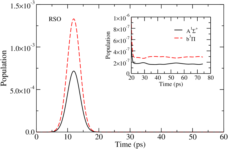
Figure 13: The total populations $P_{i}(t)$ of the excited A ${}^{1}\Sigma^{+}$ and b ${}^{3}\Pi$ electronic states during the RSO pump pulse, relative to the ground-state population. The fractions of the population that remain in the excited states after the pulse are shown in the inset.

The overall populations of the two electronically excited states, $P_{i}(t)$, are shown in Fig. 13 for the RSO case. They reach a maximum near $\tau_{\rm p}$ = 12.0 ps. Before the end of the pump pulse, most of the population returns to the initial continuum state. This corresponds to coherent transients Allen and Eberly (1974) which are off-resonant and can be excited only during the pulse. Only a small amount ($\sim 5\times 10^{-7}$) remains in the vibronic levels of the coupled excited states (as shown in the inset of Fig. 13). This population continues to oscillate between the two electronically excited states due to the nonadiabatic coupling. Such oscillations have also been observed for Rb₂ Koch et al. (2006b); Mur-Petit et al. (2007). The results for the ASO case are qualitatively similar, but reduced by about a factor of 2 because of the larger detuning from the atomic line.

Detailed information about the population of the individual vibronic levels $v^{\prime}$ can be obtained from the projection of the excited wavepacket onto excited-state vibronic levels $P^{v^{\prime}}_{\rm e}(t)$. Many vibronic levels are excited transiently during the pulse, but only levels with $v^{\prime}=363$ to 370 remain significantly populated after the pulse. The final populations of the individual near-resonant vibronic levels are shown in Fig. 14, with the time-dependence of the populations during the pulse shown in the insets. The final populations peak near $v^{\prime}$ = 365 in both cases, but with variations arising from differences in FCFs and for levels that are further off-resonance. It is noteworthy that $v^{\prime}=365$ itself is almost unpopulated in the ASO case: it has a very small FCF because it resides on the upper adiabatic curve and has very little probability density near the outermost turning point. In the RSO case, all the levels have significant upper-state character: in this case the anomalously low population of $v^{\prime}$ = 367 occurs because the maximum of the last peak of the eigenfunction corresponds to a node in the initial ground-state wavefunction at $R\sim 34.7\ a_{0}$.

In order to determine how many molecules are formed per photoassociation pulse, it is necessary to average over the final excited-state populations obtained from all thermally populated initial scattering states Koch et al. (2006d). The averaging procedure relates the scattering states employed in the calculations to the actual volume of the trap. The absolute number of molecules is limited by the probability density of atoms pairs near the Condon radius, i.e. by the population within the ‘photoassociation window’. While the exact value depends on the details of the potential, and in particular on the scattering length, an order-of-magnitude estimate can be obtained by comparing simulations for RbCs and Rb₂ using a similar scattering length, the same size of the grid and an identical initial state. In order to compare to the results for Rb₂ Koch et al. (2006b, d), we have repeated the simulation for RbCs shown in Fig. 13 using a grid of 20000 a₀ and an initial state with scattering energy corresponding to 100 $\mu$K. The final excited-state norm of $1.1\times 10^{-7}$ is about two orders of magnitude smaller than for Rb₂ (cf. Table I of Ref. Koch et al., 2006b), where about one molecule per pulse is predicted for $10^{8}$ atoms at a density of $10^{-10}$ cm^-3 Koch et al. (2006d). The reduced photoassociation yield of a $1/R^{6}$ potential compared to a $1/R^{3}$ potential requires a significantly higher density and/or a larger number of atoms to produce a comparable population of ground-state molecules.

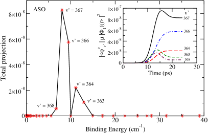
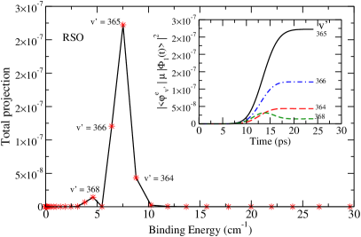
Figure 14: The final projections $P_{\rm e}^{v^{\prime}}(t)$ of the wavepacket onto the excited-state vibronic eigenfunctions as a function of their binding energies. Significant populations of molecules are formed in vibronic levels $v^{\prime}=363$ to 370. The time-dependence during the pulse is shown in the insets for the levels with the largest final population. Left-hand panel: results obtained with asymptotic spin-orbit coupling (ASO) Right-hand panel: results obtained with $R$-dependent spin-orbit coupling (RSO).

V.5 Formation of ultracold ground-state RbCs molecules

Some very loosely bound ground-state vibrational levels are populated directly by the pump pulse in processes involving more than one photon, but a dump pulse is required to populate more deeply bound levels. The dump pulse is activated after an appropriate time delay, when a substantial amount of the wavepacket has reached the short-range region where there is significant overlap with deeply bound levels of the ground electronic state. Since coherent effects between the pump and dump pulses can be neglected, the pump and dump pulses are treated separately. The excited-state population is normalized to one after the pump pulse in order to have a direct correspondence between the populations calculated and the probability of formation of ground state molecules.

It is useful to inspect the probability density distribution of the excited-state wavepackets as a function of time. Snapshots of the A ${}^{1}\Sigma^{+}$ component of the wavepackets for a few representative times are shown in Fig. 15 for both the ASO and RSO cases. The wavepacket is initially quite similar in the two cases and starts to move inwards under the influence of the long-range potential, slightly faster in the ASO case because of the larger detuning from the atomic line. However, a major difference arises after the wavepackets reach the crossing point between the diabatic curves. The ASO wavepacket remains almost entirely on the lower adiabatic curve, and thus has mostly triplet character inside $10\,a_{0}$. By contrast, the RSO wavepacket is made up of levels of mixed upper and lower-state character and there is a large buildup of singlet probability density near the inner turning point. This reaches a maximum at about 26 ps. Movie of the propagation of the A ${}^{1}\Sigma^{+}$ and b ${}^{3}\Pi$ components of the wavepackets are.

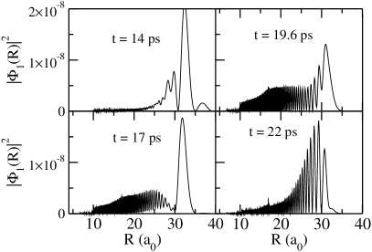
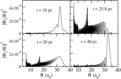
Figure 15: Snapshots of the A ${}^{1}\Sigma^{+}$ component of the wavepackets at different times after the pump pulse. Left-hand panels: results obtained with asymptotic spin-orbit coupling (ASO). Right-hand panels: results obtained with $R$-dependent spin-orbit coupling (RSO).

Figure 16: Movie showing the A ${}^{1}\Sigma^{+}$ and b ${}^{3}\Pi$ component of the wavepackets as a function of time for the asymptotic spin-orbit coupling (ASO) coupling function. [Animated gif file movieASO.gif]

Figure 17: Movie showing the A ${}^{1}\Sigma^{+}$ and b ${}^{3}\Pi$ component of the wavepackets as a function of time for the $R$-dependent spin-orbit coupling (RSO) coupling function. [Animated gif file movieRSO.gif]

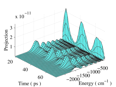
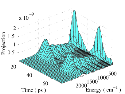
Figure 18: The time-dependence of the projections $P_{\rm g}^{v^{\prime\prime}}(t)$ of the wavepackets onto the vibrational levels of the ground electronic state. Left-hand panel: results obtained with asymptotic spin-orbit coupling (ASO). Right-hand panel: results obtained with $R$-dependent spin-orbit coupling (RSO).

The parameters of the dump pulse are optimized by considering the overlap of the excited-state wavepacket with the vibrational levels of the ground electronic state, $P_{\rm g}^{v^{\prime\prime}}(t)$. Fig. 18 shows this overlap as a function of time and binding energy. It may be seen that the RSO wavepacket has significant overlap with vibrational levels of the ground electronic state bound by up to about 1500 cm^-1. The overlap is about 2 orders of magnitude smaller in the ASO case because of the lack of population near the inner turning point. This arises from the weaker nonadiabatic coupling in the ASO case, which in turn arises from the stronger spin-orbit coupling near the crossing point. The time-dependence of the overlap is also rather different in the ASO case, both because of the larger detuning and because any population that does arise on the upper adiabatic curve is trapped there.

After examining the overlaps for different ground-state vibrational levels, we chose to de-excite the RSO wavepacket to level $v^{\prime\prime}=54$ with binding energy 1435.13 cm^-1 (shown in Fig. 1). A narrow-bandwidth pulse with temporal width 1 ps, detuned 1427.61 cm^-1 to the blue of the pump pulse, is employed to achieve transfer into this single vibrational level (because the excited-state wavepacket itself has a binding energy of 7.5 cm^-1. As may be seen in Fig. 19, the overlap function for this particular vibrational level has a local maximum at $t\sim 25.8$ ps. The time delay between the pump and dump pulses is therefore chosen to give the maximum of the dump pulse at $t_{\rm d}=25.8$ ps, corresponding to a time delay of 13.8 ps, as shown in Fig. 12. This is in reasonably good agreement with the classical prediction of 12 ps for a detuning of 7 cm^-1 in Table 1.

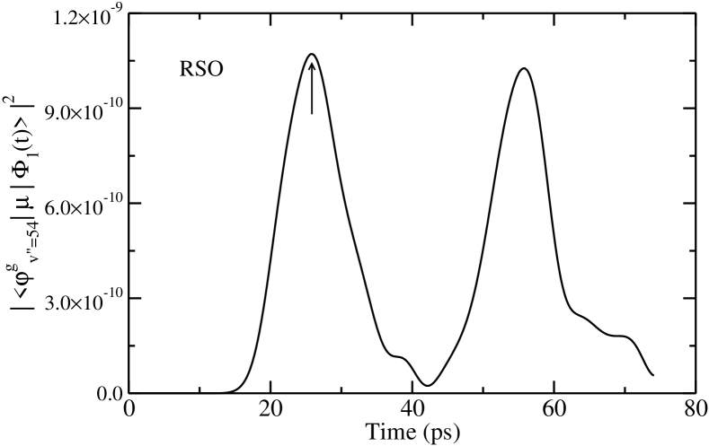
Figure 19: The projection of the excited-state wavepacket onto the $v^{\prime\prime}=54$ vibrational level of the ground electronic state. The time indicated by the arrow is the maximum of the dump pulse ($t_{\rm d}$).

The final ground-state population $P_{\rm g}^{54}(t)$ is shown in Fig. 20 as a function of the dump pulse energy. The renormalisation applied after the pump pulse removes any population that is already in the ground electronic state before the dump pulse. Since the dump pulse is resonant only with the bound $v^{\prime\prime}$ = 54 ground-state level, and the ground-state vibrational spacing of about 37 cm^-1 is much larger than the bandwidth of the pulse, the population of the $v^{\prime\prime}$ = 54 level is the same as the total ground-state population. The maximum population transfer is obtained for a pulse of energy $\sim$ 9 $\mu$J. We repeated the dump calculation for the ASO wavepacket (with a modified laser frequency and a slightly different time delay to correspond with the maximum in Fig. 18) and verified that the population of ground-state molecules is about two orders of magnitude smaller.

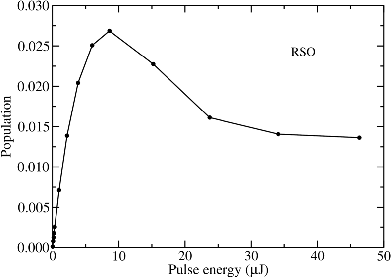
Figure 20: Fraction of the excited-state population transferred to the $v^{\prime\prime}$ = 54 level of the X ${}^{1}\Sigma^{+}$ ground state as a function of the dump pulse energy for a time delay of 13.8 ps.

Ground-state RbCs molecules bound by as much as 1500 cm^-1 can be formed because there is good Franck-Condon overlap of the excited-state wavepacket with deeply bound vibrational levels. Similar studies on the homonuclear Rb₂ molecule Koch et al. (2006b); Pechkis et al. (2007) have shown that excited Rb₂ molecules can be efficiently dumped to create ground-state vibrational levels bound by only about 10 cm^-1. For Rb₂ the wavepacket showed significant peaking of singlet population at the outer tuning point of the upper adiabatic curve but not at its inner turning point as in RbCs. The time delay used for Rb₂ was 81.5 ps with a detuning of 4.1 cm^-1 from the atomic line.

As commented above, the levels of Rb₂ do show strong nonadiabatic mixing between the upper and lower adiabatic states. In view of this, it is important to understand why RbCs shows much more buildup of singlet character near the inner turning point than Rb₂. The reason for this is that Rb₂ has an $R^{-3}$ potential at long range, so that the vibrational wavefunctions of states near dissociation are more strongly concentrated at the outer turning point. Because of this, even population that is transferred to the upper adiabatic state by nonadiabatic coupling has a smaller amplitude near the inner turning point and is less effective in allowing deexcitation to deeply-bound states.

We also note that, because of the small FC factors for deexcitation, only about 3% of the excited-state RbCs population can be transferred to the desired deeply bound ground-state vibrational level, whereas almost 50% of the excited Rb₂ population can be transferred to the ground state using much less dump pulse energy (Fig. 11 of Koch et al. (2006b)). The overall efficiency of the scheme considered here is limited by the fraction of the initial ground-state population that is transferred to the excited state. One possible way to enhance it would be by Feshbach-optimised photoassociation Pellegrini et al. (2008).

VI Conclusions

We have studied the possibility of using photoassociation with laser pulses to produce deeply bound RbCs molecules in the electronic ground state. We have also explored the differences between photoassociation processes for RbCs and Rb₂ in order to understand the consequences of the different long-range potentials in excited states of heteronuclear and homonuclear molecules.

The difference between $R^{-6}$ potentials for heteronuclear molecules and $R^{-3}$ potentials for homonuclear molecules produces several important effects. First, the Franck-Condon factors for excitation are smaller in the heteronuclear case, though they die off more slowly with detuning from the atomic line. Secondly, the time taken for a wavepacket produced on the upper state to evolve from long to short range is significantly shorter for a heteronuclear molecule than for a homonuclear molecule of similar mass at the same detuning. We give a simple semiclassical expression relating the time delay to the detuning and the coefficients governing the long-range potential.

We have also explored the dependence of Franck-Condon factors on the scattering lengths for both the ground state and the excited state. The Franck-Condon factors oscillate as a function of detuning, with faster oscillations for RbCs than for Rb₂. Adjusting the ground-state scattering length alters the positions of the peaks in the Franck-Condon factors as a function of detuning, while adjusting the excited-state scattering length leaves the oscillations unchanged but shifts the vibrational levels within them.

We have carried out wavepacket calculations to explore the quantum dynamics of RbCs on $0^{+}$ excited states formed by coupling the A ${}^{1}\Sigma^{+}$ and b ${}^{3}\Pi$ electronic states. The diabatic potential curves for the A and b states cross near $R=10\,a_{0}$. The dynamics are strongly affected by the magnitude of the spin-orbit coupling. If the spin-orbit coupling function is held constant at its asymptotic value, the dynamics takes place almost independently on the upper and lower adiabatic curves. Under these circumstances the wavepacket has almost entirely triplet character at short range and the Franck-Condon factors for deexcitation to deeply-bound levels of the ground state are very poor. However, if the spin-orbit coupling is given a more realistic experimentally derived form Fellows and Bergeman (2007) that has a smaller value near the crossing point, the dynamics are strongly nonadiabatic. A substantial part of the population is transferred to the upper adiabatic state, which has singlet character at short range. This allows efficient deexcitation to levels of the ground electronic state bound by up to 1500 cm^-1.

The behavior observed for RbCs may be contrasted with that for Rb₂ Koch et al. (2006b); Pechkis et al. (2007). Rb₂ has only slightly weaker nonadiabatic coupling but deexcitation is favored to ground-state levels bound by up to only 10 cm^-1. The difference in this case arises from the different long-range potentials: for Rb₂ there is an $R^{-3}$ potential at long range and the density distribution for the upper-state levels is dominated by the outer turning point of the upper adiabatic curve. From the outer turning point, the Franck-Condon factors favor deexcitation to relatively weakly-bound levels of the ground electronic state.

An important new insight from the present work is that the combination of strong nonadiabatic coupling with a $1/R^{6}$ potential produces mixed vibrational levels with significant singlet density both at long range (which facilitates initial photoassociation) and near the inner turning point of the singlet state (which facilitates deexcitation to form deeply bound ground-state levels). This allows ‘$R$-transfer’ in a way which does not occur for homonuclear species. This phenomenon is also expected to be present in other heavy heteronuclear dimers such as KRb or KCs. It is easily identified spectroscopically in the level spacings or rotational constants and will play an important role that is not confined to photoassociation, for example in stimulated Raman adiabatic pumping (STIRAP) experiments to form deeply bound states.

Our study of pump-dump photoassociation was motivated by the search for a coherent scheme for forming deeply bound molecules where the dump pulse does not destroy the molecules that were created by the pump pulse. STIRAP is another candidate for this, and has recently been applied successfully to transfer near-dissociation Cs₂ Danzl et al. (2008b, a) and KRb Ospelkaus et al. (2008); Ni et al. (2008) molecules to deeply bound states. However, STIRAP requires a few well-separated levels in order to fulfill the adiabaticity condition and this requirement is not met by the quasi-continuum of a MOT. This might be circumvented by applying STIRAP after a photoassociation pump pulse, in order to optimize the dump step. In other words the pump pulse prepares a coherent state which in a two-level picture replaces the upper level, while the target ground-state vibrational level plays the role of the lower level. Several realizations of adiabatic passage in two-level systems exist, such as Stark-chirped rapid adiabatic passage (SCRAP) Yatsenko et al. (1999); Rickes et al. (2000) and retroreflection-induced bichromatic adiabatic passage (RIBAP) Yatsenko et al. (2003); Conde et al. (2005). The underlying concept of these schemes is to induce a crossing of the two levels and an adiabatic or diabatic passage of the induced crossing. In our case the adiabatic passage would need to proceed on a timescale long compared to the vibrational motion of the wavepacket (about 40 ps) and short compared to spontaneous emission (about 30 ns). However, to see whether replacing the picosecond dump pulse by an adiabatic passage scheme is feasible and whether it allows the dump efficiency to be increased above the 3% reported here is beyond the scope of the present study.