Semiclassical framework for the calculation of transport anisotropies

Abstract

We present a procedure for finding the exact solution to the linear-response Boltzmann equation for two-dimensional anisotropic systems and demonstrate it on examples of non-crystalline anisotropic magnetoresistance in a system with spin-orbit interaction. We show that two decoupled integral equations must be solved in order to find the non-equilibrium distribution function up to linear order in the applied electric field. The examples are all based on the Rashba system with charged magnetic scatterers, a system where the non-equilibrium distribution function and anisotropic magnetoresistance can be evaluated analytically. Exact results are compared to earlier widely-used approximative approaches. We find circumstances under which approximative approaches may become unreliable even on a qualitative level.

I Introduction

The change of electric resistance upon varying magnetization direction is an old and well-known phenomenonThomson (1857); Döring (1938); Jaoul et al. (1977) with applications in spintronics.Zutic et al. (2004); Fabian et al. (2007) Although the experimental observation of this anisotropic magnetoresistance (AMR) is rather direct — first accomplished as early as 1857 — its theoretical understanding is far from being complete. It has long been clear that the phenomenon arises from the combined effects of magnetization and spin-orbit interaction. Disregarding the crystalline anisotropic background, the magnetization-broken symmetry between two chosen directions and unequal resistivities along these has been described within different models. In transition metal ferromagnets, the anisotropy was ascribed to asymmetric scattering due to different parts of the spin-orbit interaction $\vec{L}\cdot\vec{S}=\frac{1}{2}(L_{-}S_{+}+L_{+}S_{-})+L_{z}S_{z}$ and the mechanisms considered were dubbed the $L_{-}S_{+}$ model,Smit (1951) $L_{z}S_{z}$ model,Berger (1964) or a combination of both.McGuire and Potter (1975); Jaoul et al. (1977) Later, when computational power became sufficient for such task, ab initio calculations were performedBanhart and Ebert (1995) for permalloy and reached a good agreement with experiments. However, no direct link between the ab initio and the model calculations listed above has been established, probably due to rather complex band structures involved. On the other hand, such link between microscopic calculations and a simple physical model was recently found in the diluted magnetic semiconductorRushforth et al. (2008, 2007) (Ga,Mn)As whose band structure is much simpler.

Despite the long history of the AMR research, the question has not been answered to date of how a rigorous transport formalism for anisotropic systems should be formulated. Instead, the transport anisotropy has often been discussed only in terms of the asymmetry in scattering amplitudes between two states on the Fermi surface. Current availability of materials with relatively simple band structure motivates the quest for more precise theories of AMR. The present article discusses how the semiclassical Boltzmann equation should be solved in anisotropic systems, using an example of the model two-dimensional (2D) electron system. This allows us to put the previous approximations on rigorous grounds.

The conductivity of a given solid in the regime of linear response to the electric field $\vec{\cal E}$ can be evaluated within the semiclassical picture once we have found the distribution function satisfying the Boltzmann equation. In the literature, this non-equilibrium distribution function is approximated in several ways. The relaxation time approximation (RTA) relies on calculating the transport relaxation time $\tau$ from the scattering amplitudes $w(\vec{k},\vec{k}^{\prime})$ between two states on the Fermi surface using

$$\frac{1}{\tau}=\int\frac{d^{2}k^{\prime}}{(2\pi)^{2}}w(\vec{k},\vec{k}^{\prime})\big{[}1-\cos\vartheta_{\vec{k}\vec{k}^{\prime}}\big{]}\,.$$ (1)

For isotropic systems, where $w$ depends only on the angle $\vartheta_{\vec{k}\vec{k}^{\prime}}$ between $\vec{k}$ and $\vec{k}^{\prime}$, the integral (1) does not depend on the direction of $\vec{k}$ and the RTA provides in fact the exact solution to the Boltzmann equationAshcroft and Mermin (1976). The scattering rate $1/\tau$ depends only on energy and it is constant on the whole Fermi surface once the Fermi energy is fixed.

For anisotropic systems, keeping Eq. (1) in use produces $1/\tau$ that depends on the direction of $\vec{k}$. The non-equilibrium distribution function constructed utilising the RTA and Eq. (1) may capture some aspects of the transport anisotropies but it is certainly not precise. This approximative approach underlies for example our previous calculationsRushforth et al. (2007) or those of McGuire and PotterMcGuire and Potter (1975) and we refer to it as to the “$1/\tau$ approach”.

An improvement was proposed by Schliemann and Loss.Schliemann and Loss (2003) In what we will call the “$1/\tau^{\parallel}\,\&\,1/\tau^{\perp}$ approach”, they use, according to their notation, Eq. (1) to calculate $1/\tau^{\parallel}(\vec{k})$, and they provide an explicit formula for the non-equilibrium distribution in terms of this quantity and of

$$\frac{1}{\tau^{\perp}(\vec{k})}=\int\frac{d^{2}k^{\prime}}{(2\pi)^{2}}w(\vec{k},\vec{k}^{\prime})\sin\vartheta_{\vec{k}\vec{k}^{\prime}}\,.$$ (2)

In our article, we argue that in a general case the non-equilibrium distribution function cannot be exactly calculated by just evaluating two integrals such as Eqs. (1,2) for each $\vec{k}$-point of the Fermi surface separately. Instead, an integral equation must be solved that determines the whole non-equilibrium distribution at once. In Section II, we describe this exact “integral equation approach” to transport in anisotropic 2D systems and then, in Section III, we use a simple model system to illustrate how the procedure works. For this purpose we introduce the Rashba Hamiltonian combined with a scattering potential due to randomly distributed charged and ferromagnetically ordered impurities. In this model, the AMR results from the spin-orbit coupled band structure and the broken time-reversal symmetry of the scattering potential.Rushforth et al. (2007) We explicitly calculate exact non-equilibrium distribution functions for several specific realizations of this model, starting from the ones with simple solutions and then proceeding to the more complex case. Throughout Section III we compare our distribution functions and AMRs to results of the other two approximative approaches. Section IV concludes the main body of the article by discussing the relevance of our model calculations for the AMR in magnetic semiconductors and by summarizing the key elements of the theoretical framework we have developed. The Appendices contain details of our calculations and also a more thorough description of the $1/\tau$ and $1/\tau^{\parallel}\,\&\,1/\tau^{\perp}$ approaches.

II The framework

Our central goal is to obtain the distribution function $f=f(\vec{k},\vec{{\cal E}})$ of a conductor displaced from equilibrium by a small bias represented by a weak homogeneous electric field $\vec{{\cal E}}$. We start with the familiar form of the Boltzmann equation in 2D

$$-e\vec{{\cal E}}\cdot\vec{v}(\vec{k})(-\partial_{\epsilon}f_{0})=\int\frac{d^{2}k^{\prime}}{(2\pi)^{2}}w(\vec{k},\vec{k}^{\prime})[f(\vec{k},\vec{\cal E})-f(\vec{k}^{\prime},\vec{\cal E})]$$ (3)

for a steady state of a spatially homogeneous system. Derivation of this equation is described for instance in Ref. Schliemann and Loss, 2003. Equation (3) is valid up to linear order in $|\vec{{\cal E}}|$ and it assumes small deviations of $f(\vec{k},\vec{E})$ from the equilibrium distribution $f_{0}=f_{0}(\vec{k})$. The velocity $\vec{v}=(1/\hbar)\nabla_{k}\epsilon_{\vec{k}}$ is implied by the band dispersion $\epsilon_{\vec{k}}$, and $e$ is the charge of carriers. The scattering rate $w$ (per unit area of the reciprocal space) from the state $\vec{k}$ to $\vec{k}^{\prime}$ needs to be specified according to the microscopic origin of the scattering; specific examples can be found in Appendix .1 or in Eq. (38) of Ref. Schliemann and Loss, 2003. For now we only assume that the scattering is elastic, that is $w(\vec{k},\vec{k}^{\prime})\propto\delta\big{(}\epsilon_{\vec{k}}-\epsilon_{\vec{k}^{\prime}}\big{)}$. Focusing on the AMR, we do not include anomalous termsSinitsyn et al. (2007); Sinitsyn (2008) like the coordinate shift related to the side jump in the anomalous Hall effect into the right hand side of Eq. (3). Equation (3) can be applied to multi-band systems where $\vec{k}$ is replaced by a compound index containing the wavevector and band index and the integral by integration over the wavevector and summation over bands.

The solution to Eq. (3) is a function both of $\vec{k}$ and $\vec{{\cal E}}$. Focusing first on the latter, we can write it as Taylor series

$$f(\vec{k},\vec{{\cal E}})=f_{0}+{\cal E}_{x}\partial_{{\cal E}_{x}}f+{\cal E}_{y}\partial_{{\cal E}_{y}}f+\sum_{ij}{\cal E}_{i}{\cal E}_{j}\partial_{{\cal E}_{i}}\partial_{{\cal E}_{j}}f+\ldots$$ (4)

Being interested only in the linear order of the electric field components $({\cal E}_{x},{\cal E}_{y})$, we will truncate the series after the third term. For the simplicity of notation, we will now assume that the band structure is isotropic, $\epsilon_{\vec{k}}=\epsilon_{k}$ and $-\delta_{\epsilon}f_{0}=\delta(\epsilon-\epsilon_{k})$. The anisotropy can still pervade into the transport via $w$, for instance due to anisotropic scatterers. The more general Boltzmann equation for anisotropic bands is treated in Appendix .7.

We define two angles $\phi$, $\theta$ as $\vec{{\cal E}}={\cal E}(\cos\theta,\sin\theta)$ and $\vec{k}=k(\cos\phi,\sin\phi)$ and Eq. (4) becomes

$$f(\phi,\theta)-f_{0}={\cal E}\big{(}A(\phi)\cos\theta+B(\phi)\sin\theta\big{)}$$ (5)

after the truncation, where $A(\phi)=\partial_{{\cal E}_{x}}f$ and $B(\phi)=\partial_{{\cal E}_{y}}f$. The non-equilibrium distribution is now expressed in terms of two functions of $\phi$ which must, according to Eq. (3) with Eq. (5) inserted, fulfil

$$\cos(\theta-\phi) = \left[\bar{w}(\phi)a(\phi)-\int d\phi^{\prime}\ w(\phi,\phi^{\prime})a(\phi^{\prime})\right]\cos\theta+$$ (6)

$$\hskip-28.45274pt+\left[\bar{w}(\phi)b(\phi)-\int d\phi^{\prime}\ w(\phi,\phi^{\prime})b(\phi^{\prime})\right]\sin\theta\,.$$

We define here $A(\phi)\equiv-ev(-\partial_{\epsilon}f_{0})\,a(\phi)$, $B(\phi)\equiv-ev(-\partial_{\epsilon}f_{0})\,b(\phi)$, and $\bar{w}(\phi)=\int d\phi^{\prime}\ w(\phi,\phi^{\prime})$, where $w(\phi,\phi^{\prime})=(2\pi)^{-2}\int k^{\prime}\,dk^{\prime}w(\vec{k},\vec{k}^{\prime})$ now includes the original transport scattering rate $w(\vec{k},\vec{k}^{\prime})$ and also the density of states.

The integral equation (6) with two variables $\phi,\theta$ can be decomposed into two independent integral equations

$$\cos\phi = \bar{w}(\phi)\,a(\phi)-\int d\phi^{\prime}w(\phi,\phi^{\prime})a(\phi^{\prime})$$ (7)

$$\sin\phi = \bar{w}(\phi)\,b(\phi)-\int d\phi^{\prime}w(\phi,\phi^{\prime})b(\phi^{\prime})$$ (8)

whose solutions $a(\phi)$, $b(\phi)$ inserted into Eq. (5) yield the exact solution of the Boltzmann equation (3) up to the linear order in ${\cal E}$.

The two decoupled inhomogeneous Fredholm equationsfredholm of the second kind (7,8) can be most conveniently solved in terms of Fourier series. For special choices of $w(\phi,\phi^{\prime})$ or band structure anisotropy (see Appendix .7), the series may contain only few terms and reduce to an ansatz for $f(\phi,\theta)$ such as Eq. (15) in Ref. Trushin and Schliemann, 2007. We explain the general procedure how to solve Eqs. (7,8) on three examples below.

III Three examples with Rashba system

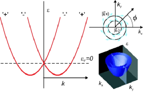
To illustrate how the above outlined procedure works, we choose the $2\times 2$ Rashba HamiltonianFabian et al. (2007) in the basis of plane waves

$$\hat{H}=\frac{\hbar^{2}k^{2}}{2m}+\lambda(k_{x}\sigma_{y}-k_{y}\sigma_{x})\,,$$ (9)

where $\sigma_{x,y}$ are the Pauli matrices, and $\lambda$ is the Rashba parameter. In addition to Eq. (9), we consider scattering on dilute charged magnetic impuritiesRushforth et al. (2007, 2008) described by the operator $\hat{V}$,

$$\hat{V}/V_{0}=\alpha+\sigma_{x}=\left(\begin{array}[]{cc}\alpha&1\\ 1&\alpha\end{array}\right)\,,$$ (10)

that is impurities containing short range electric and ferromagnetically ordered magnetic potentials. The quantity $\alpha$ is the (dimensionless) strength of the electric part, relative to the magnetic part, of the ’electro-magnetic scatterer’ whose magnetic moment was chosen to be along the $x$ direction. The magnitude $V_{0}$ and other aspects of this model are discussed in Section IV and Appendices .1 and .2.

We now calculate the non-equilibrium Boltzmann distribution function $f(\vec{k},\vec{\cal E})=f(\phi,\theta)$ for this model in several special cases. To facilitate relevant comparison between the $1/\tau$ and $1/\tau^{\parallel}\,\&\,1/\tau^{\perp}$ approaches and the exact integral equation approach of Section II, we calculate $f(\phi,\theta)$ and evaluate the AMR within the approximative approaches as well.

III.1 Single band and magnetic scatterers

The first special case of the model above concerns purely magnetic scatterers ($\alpha=0$) in the situation when the Fermi energy cuts the spectrum of the Rashba Hamiltonian (9) precisely at the $k=0$ degeneracy point ($\epsilon_{F}=0$ in Fig. 1). We further disregard this single point of the Fermi surface and consider only the ’+’ band. This case offers the simplest way to explain the calculation of $f$ outlined in Section II.

The dimensionless scattering probability corresponding to $\hat{V}$ of Eq. (10) is

$$w(\phi,\phi^{\prime})/K=\frac{1}{2}[1-\cos(\phi+\phi^{\prime})]\,.$$ (11)

This result, including the dimensionful prefactor $K$, is derived using the Fermi golden rule in Appendix .1 and .2. Although $w(\phi,\phi^{\prime})$ does not explicitly depend on the Rashba parameter $\lambda$, the presence of the spin-orbit coupling, combined with the symmetry breaking scattering potential, has the crucial implication that $w$ depends on absolute values of angles $\phi$ and $\phi^{\prime}$. This leads to the non-zero anisotropy of the magnetotransport, in contrast to the isotropic case in which $w(\phi,\phi^{\prime})$ depends only on the relative angle $\phi-\phi^{\prime}$ between the incoming and outgoing momenta. The total scattering probability, implied by Eq. (11), reads

$$\bar{w}(\phi)=K\pi\,.$$ (12)

Note that despite the independence of $\bar{w}$ on $\phi$ in the special case considered in this subsection the resulting relaxation times and conductivity are indeed anisotropic.

Figure 1: Summary of the Rashba model defined by the Hamiltonian (9). The three-dimensional plot shows energy dispersions; its cross section along one (arbitrary) direction in the $\vec{k}$-space is also shown. The spin textures for the pair of eigenstates $|\vec{k}+\rangle$ and $|\vec{k}-\rangle$ for each $\vec{k}$ at the respective Fermi surfaces with $\epsilon_{F}>0$ are shown on the top. Unlike the diameters of the $+$ and $-$ Fermi surfaces, the eigenstates (spin textures) are independent of the Fermi energy $\epsilon_{F}$, according to Eq. (54).

We will now look for the solution $a(\phi)$ to Eq. (7) in the form of Fourier series

$$a(\phi) = a_{0}+a_{c1}\cos\phi+a_{c2}\cos 2\phi+\ldots+$$ (13)

$$\phantom{a_{0}}+a_{s1}\sin\phi+a_{s2}\sin 2\phi+\ldots\,.$$

Owing to the trivial form of $w(\phi,\phi^{\prime})$ (of its Fourier spectrum) the integral in Eq. (7) can be readily calculated and Eq. (7) assumes the following form:

$$\displaystyle\frac{1}{\pi K}\cos\phi = \frac{3}{2}a_{c1}\cos\phi+a_{c2}\cos 2\phi+a_{c3}\cos 3\phi+\ldots+$$

$$+\frac{1}{2}a_{s1}\sin\phi+a_{s2}\sin 2\phi+a_{s3}\sin 3\phi+\ldots\,.$$

The only non-zero coefficients in the Fourier series (13) are therefore $a_{0}$ and $a_{c1}$. The solution of Eq. (7) then reads

$$a(\phi)=a_{0}+\frac{2/3}{\pi K}\cos\phi\,.$$ (14)

Conservation of the number of particles requires $a_{0}$ to be zero.

A completely analogous procedure applied to Eq. (8) yields a system of equations for coefficients $b_{0}$, $b_{s1}$, $b_{c1}$ which give

$$b(\phi)=\frac{2}{\pi K}\sin\phi\,.$$ (15)

The complete solution up to linear order in ${\cal E}$ to the Boltzmann equation (3) written using Eq. (5) is therefore

$$f(\phi,\theta)\!=\!f_{0}-ev{\cal E}(-\partial_{\epsilon}f_{0})\frac{2}{\pi K}\bigg{[}\frac{1}{3}\cos\theta\cos\phi+\sin\theta\sin\phi\bigg{]}\,.$$ (16)

Let us now compare this result to the approximate approaches outlined in the Introduction. The non-equilibrium distribution in the $1/\tau$ approach is (see Appendix .3)

$$f(\phi,\theta)-f_{0} = -ev{\cal E}(-\partial_{\epsilon}f_{0})\frac{2}{\pi K}\times$$

$$\hskip-5.69054pt\times\left[\cos\theta\frac{\cos\phi}{3-2\sin^{2}\phi}+\sin\theta\frac{\sin\phi}{3-2\sin^{2}\phi}\right]\,,$$

while in the $1/\tau^{\parallel}\,\&\,1/\tau^{\perp}$ approach (see Appendix .4), we obtain

$$f(\phi,\theta)-f_{0} = -ev{\cal E}(-\partial_{\epsilon}f_{0})\frac{2}{\pi K}\times$$

$$\times\left[\cos\theta\frac{3\cos\phi+2\sin^{2}\phi(1-\cos\phi)}{9+4\sin^{4}\phi-8\sin^{2}\phi}+\right.$$

$$\hskip 19.91684pt\left.+\sin\theta\frac{3\sin\phi(1-\cos\phi)-2\sin^{3}\phi}{9+4\sin^{4}\phi-8\sin^{2}\phi}\right]\,.$$

Distribution functions in Eqs. (16,III.1,III.1) are significantly different. To quantify the differences, we use these three distribution functions to calculate the AMR, defined as

$$\mbox{AMR}=-\frac{\sigma_{xx}-\sigma_{yy}}{\sigma_{xx}+\sigma_{yy}}$$ (19)

and having the meaning of the (relative) difference in resistivity for current flowing parallel and perpendicular to the direction of the scatterer’s magnetic moment, respectively. The conductivities are calculated from the current implied by the non-equilibrium distribution $f(\vec{k},\vec{\cal E})$

$$\vec{j}(\vec{\cal E})=\int\frac{d^{2}k}{(2\pi)^{2}}e\vec{v}(\vec{k})\,f(\vec{k},\vec{\cal E})\,,$$ (20)

i.e., as $\sigma_{xx}=j(\theta=0)/{\cal E}$ and $\sigma_{yy}=j(\theta=\pi/2)/{\cal E}$ where $j(\theta)=\int d\phi f(\phi,\theta)|\vec{v}|\cos(\phi-\theta)$.

The AMR value of $1/2$, obtained from the exact non-equilibrium distribution function in Eq. (16), is markedly different from the results of the approximative approaches. The $1/\tau$ approach underestimates the AMR by almost a factor of two ($\mbox{AMR}\approx 0.27$), and the $1/\tau^{\parallel}\,\&\,1/\tau^{\perp}$ approach predicts even a wrong sign ($\mbox{AMR}\approx-0.11$).

Before we proceed to comparing the three approaches on other realizations of our model disordered 2D system, let us make a remark about the distribution functions above. The non-equilibrium part of the distribution function in Eq. (III.1) was obtained as $-e\vec{v}\cdot{\cal\vec{E}}(-\partial_{\epsilon}f_{0})\tau(\phi)$ with $\vec{v}\cdot\vec{\cal E}=v{\cal E}\cos(\theta-\phi)$ and $\tau(\phi)=(2/\pi K)(3-2\sin^{2}\phi)^{-1}$ as derived in Appendix .3. Analogous factorization of the bracket in Eq. (III.1) or Eq. (16) is not possible, reflecting the fact that no scalar relaxation time can be attributed to a given $\vec{k}$–state in these approaches. However, the $1/\tau^{\parallel}\,\&\,1/\tau^{\perp}$ approach still unambiguously assigns relaxation-rate-like quantities, a pair of (not necessarily positive) values $1/\tau^{\parallel}(\vec{k}),1/\tau^{\perp}(\vec{k})$, to each $\vec{k}$-state, independent of the electric field direction (determined by $\theta$; see Appendix .4). It remains an open question whether also the exact solution of the Boltzmann equation, such as Eq. (16), can be meaningfully interpreted in terms of $\theta$–independent quantities related to scattering.

III.2 Single band and electro-magnetic scatterers

We now extend results of the previous section by relaxing the condition $\alpha=0$, that is we consider the complete scatterer with electric and magnetic parts of its potential added up coherently, as defined by Eq. (10). The extension is straightforward although the algebra involved is richer than for the previous model. The dimensionless scattering probability $w(\phi,\phi^{\prime})/K$ and $\bar{w}(\phi)$ are

$$\begin{array}[]{rcl}w(\phi,\phi^{\prime})/K&=&\frac{1}{2}\big{[}1-\cos(\phi+\phi^{\prime})+\alpha^{2}\big{(}1+\cos(\phi-\phi^{\prime})\big{)}\big{]}\\[2.84526pt] &&+\alpha(\sin\phi+\sin\phi^{\prime})\\[5.69054pt] \bar{w}(\phi)&=&\pi K(1+\alpha^{2}+2\alpha\sin\phi)\,,\end{array}$$ (21)

as shown in Appendices .1 and .2. Note that $\bar{w}(\phi)$ is no longer constant, which is here the direct reason of the more complex algebra needed. We again look for the solution of Eq. (7) in the form of Fourier series (13) and find that the higher order coefficients $a_{c2},a_{c3},\ldots$ are now no longer zero. Instead of Eq. (14), we get a system of an infinite number of linear equations which is not surprising, given that Eq. (7) is an integral equation in its general form.

This system of equations can be solved using a partitioning method, described in Appendix .5. Herein, we segregate the variables into three groups: $\{a_{0},a_{c1},a_{s1}\}$, $\{a_{c2},a_{c3},\ldots\}$, and $\{a_{s2},a_{s3},\ldots\}$. The first group must obey

$$\begin{array}[]{rcl}1/(\pi K)&=&(1+\alpha^{2})a_{c1}+\alpha a_{s2}+\frac{1}{2}(1-\alpha^{2})a_{c1}\\[2.84526pt] 0&=&(1+\alpha^{2})a_{s1}-\alpha a_{c2}-\frac{1}{2}a_{s1}(1+\alpha^{2})\,,\end{array}$$ (22)

and $a_{0}=0$ as in the previous Subsection. Equations (22) originate from comparing the coefficients in front of the $\cos\phi$ and $\sin\phi$ terms of Eq. (7) with Eq. (13) inserted. Separate treatment of the other two infinite systems of equations, described in Appendix .5, yields

$$a_{c2}=\left\{\begin{array}[]{l}a_{s1}\alpha\\ a_{s1}/\alpha\end{array}\right.\quad a_{s2}=\left\{\begin{array}[]{ll}-a_{c1}\alpha&\mbox{ for }|\alpha|<1\\ -a_{c1}/\alpha&\mbox{ for }|\alpha|>1\,.\end{array}\right.$$ (23)

Together, Eqs. (22,23) form a closed system for $a_{c1}$, and $a_{s1}$ which thus read

$$a_{c1}=\frac{1}{2\pi K}\times\left\{\begin{array}[]{ll}4/(3-\alpha^{2})&\mbox{ for }|\alpha|<1\\ 4/(1+\alpha^{2})&\mbox{ for }|\alpha|>1\end{array}\right.\quad a_{s1}=0\,.$$

The solution to Eq. (7) for $|\alpha|<1$ is then

$$a(\phi)=\frac{1}{2\pi K}\cdot\frac{4}{3-\alpha^{2}}\cos\phi+a_{c2}\cos 2\phi+a_{s2}\sin 2\phi+\ldots\,.$$ (24)

For the evaluation of current and AMR using Eq. (19) there is no need to know the higher order terms of $f(\phi,\theta)$ (by virtue of $\int_{0}^{2\pi}\cos\phi\cos 2\phi=0$ etc.). However, keeping all higher order terms of Eq. (13) in the derivation was necessary for obtaining the xscorrect form of Eq. (22) and also correct expressions for constants $a_{c1}$ and $a_{s1}$ at the end.

We again repeat the same procedure for Eq. (8), obtain $b(\phi)$, and finally we complete the calculation by writing down the non-equilibrium distribution function:

$$f(\phi,\theta)-f_{0} = -ev{\cal E}(-\partial_{\epsilon}f_{0})\frac{2}{\pi K}\times$$

$$\times\left[\cos\theta\frac{\cos\phi}{3-\alpha^{2}}+\ldots+\sin\theta\frac{\sin\phi}{1-\alpha^{2}}+\ldots\right]$$

for $|\alpha|<1$, while for $|\alpha|>1$ the bracket is replaced by

$$\left[\cos\theta\frac{\cos\phi}{\alpha^{2}+1}+\ldots+\sin\theta\frac{\sin\phi}{\alpha^{2}-1}+\ldots\right]\,.$$ (26)

The dots symbolize $\cos 2\phi$, $\sin 2\phi$ and higher order terms which as emphasised above do not contribute to the AMR. The divergence of this expression for $|\alpha|\to 1$ will be discussed in Section IV.

Evaluating the AMR using the distribution function (III.2,26) and Eqs. (20,19) amounts to comparing the coefficients in front of the $\cos\theta\cos\phi$ and $\sin\theta\sin\phi$ summands. We get

$$\mbox{AMR}=\frac{1}{2-\alpha^{2}}\,,\ |\alpha|<1\qquad\mbox{AMR}=\frac{1}{\alpha^{2}}\,,\ |\alpha|>1\,.$$ (27)

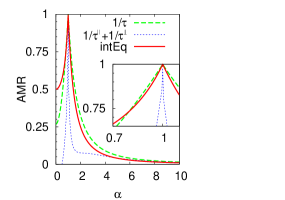
We conclude the study of the single-band model by comparing this AMR to the results of the approximate $1/\tau$ and $1/\tau^{\parallel}\,\&\,1/\tau^{\perp}$ approaches shown in Fig. 2(a). While the $1/\tau$ approach can be regarded as only quantitatively inaccurate, as already suggested by the results of the previous Subsection, the apparently more sophisticated $1/\tau^{\parallel}\,\&\,1/\tau^{\perp}$ approach yields remarkably large deviations from the exact AMR.

(a)	(b)

Figure 2: AMR as a function of the relative strength, $\alpha$, of the electric and magnetic components of the impurity potential (see Eq. (10) for the definition of $\alpha$). Dashed and dotted lines denote results of the approximative $1/\tau$ and $1/\tau^{\parallel}\,\&\,1/\tau^{\perp}$ approaches, solid line shows the exact result of the integral equation approach. (a) Single-band model, (b) two-band model with $\lambda\to 0$.

III.3 Two bands and electro-magnetic scatterers

We now consider the case when the Fermi energy is above the $k=0$ degeneracy point of the Rashba bands. Let us first explicitly write down the scheme of Sec. II for a two-band system. Considering distribution functions of the ’+’ and ’$-$’ bands, denoted by $f_{+}$ and $f_{-}$, Eq. (3) is replaced by two coupled equations

$$-e\vec{{\cal E}}\cdot\vec{v}_{+}(\vec{k})\left(-\frac{\partial f_{0}(\epsilon_{\vec{k}+})}{\partial\epsilon}\right) =$$

$$\hskip-113.81102pt=\int\frac{d^{2}k^{\prime}}{(2\pi)^{2}}\big{[}\big{(}w_{++}(\vec{k},\vec{k}^{\prime})+w_{+-}(\vec{k},\vec{k}^{\prime})\big{)}f_{+}(\vec{k})-$$

$$\hskip-71.13188pt-w_{++}(\vec{k},\vec{k}^{\prime})f_{+}(\vec{k}^{\prime})-w_{+-}(\vec{k},\vec{k}^{\prime})f_{-}(\vec{k}^{\prime})\big{]}$$

and

$$-e\vec{{\cal E}}\cdot\vec{v}_{-}(\vec{k})\left(-\frac{\partial f_{0}(\epsilon_{\vec{k}-})}{\partial\epsilon}\right) =$$

$$\hskip-113.81102pt=\int\frac{d^{2}k^{\prime}}{(2\pi)^{2}}\big{[}\big{(}w_{--}(\vec{k},\vec{k}^{\prime})+w_{-+}(\vec{k},\vec{k}^{\prime})\big{)}f_{-}(\vec{k})-$$

$$\hskip-71.13188pt-w_{--}(\vec{k},\vec{k}^{\prime})f_{-}(\vec{k}^{\prime})-w_{-+}(\vec{k},\vec{k}^{\prime})f_{+}(\vec{k}^{\prime})\big{]}\,.$$

The scattering rate $w_{fi}$ now also bears the indices of the initial ($i$) and final ($f$) band. We will abbreviate the equilibrium distributions $f_{0}(\epsilon_{\vec{k}\pm})$ by $f_{0\pm}$.

Assuming isotropic bands $\epsilon_{k+}$ and $\epsilon_{k-}$, we seek a solution of Eqs. (III.3) in the form of

$$\begin{array}[]{c}\!\!f_{+}(\phi,\theta)\!-\!f_{0}\!=\!-e{\cal E}v_{+}(-\partial_{\epsilon}f_{0+})\big{(}a_{+}(\phi)\cos\theta+b_{+}(\phi)\sin\theta\big{)}\\[5.69054pt] \!\!f_{-}(\phi,\theta)\!-\!f_{0}\!=\!-e{\cal E}v_{-}(-\partial_{\epsilon}f_{0-})\big{(}a_{-}(\phi)\cos\theta+b_{-}(\phi)\sin\theta\big{)}\end{array}$$ (29)

and the four functions $a_{\pm}(\phi)$, $b_{\pm}(\phi)$ must fulfil

$$\begin{array}[]{rcl}\cos\phi&=&\bar{w}_{+}(\phi)\,a_{+}(\phi)\\ &&\displaystyle\hskip-14.22636pt-\int d\phi^{\prime}\left[w_{++}(\phi,\phi^{\prime})a_{+}(\phi^{\prime})+w_{+-}(\phi,\phi^{\prime})a_{-}(\phi^{\prime})\right]\\ \cos\phi&=&\bar{w}_{-}(\phi)\,a_{-}(\phi)\\ &&\displaystyle\hskip-14.22636pt-\int d\phi^{\prime}\left[w_{--}(\phi,\phi^{\prime})a_{-}(\phi^{\prime})+w_{-+}(\phi,\phi^{\prime})a_{+}(\phi^{\prime})\right]\end{array}$$ (34)

$$\begin{array}[]{rcl}\sin\phi&=&\bar{w}_{+}(\phi)\,b_{+}(\phi)\\ &&\displaystyle\hskip-14.22636pt-\int d\phi^{\prime}\left[w_{++}(\phi,\phi^{\prime})b_{+}(\phi^{\prime})+w_{+-}(\phi,\phi^{\prime})b_{-}(\phi^{\prime})\right]\\ \sin\phi&=&\bar{w}_{-}(\phi)\,b_{-}(\phi)\\ &&\displaystyle\hskip-14.22636pt-\int d\phi^{\prime}\left[w_{--}(\phi,\phi^{\prime})b_{-}(\phi^{\prime})+w_{-+}(\phi,\phi^{\prime})b_{+}(\phi^{\prime})\right]\end{array}$$ (39)

where $w_{fi}(\phi,\phi^{\prime})=(2\pi)^{-2}\int k^{\prime}\,dk^{\prime}w_{fi}(\vec{k},\vec{k}^{\prime})$ and $\bar{w}_{i}(\phi)=\int d\phi^{\prime}[w_{+i}(\phi,\phi^{\prime})+w_{-i}(\phi,\phi^{\prime})]$. Note that Eqs. (34) are decoupled from Eqs. (39).

III.3.1 Evaluation of $f_{+}$ and $f_{-}$

The dimensionless scattering probabilities for the complete electro-magnetic scattering operator given by Eq. (10) are

$$\begin{array}[]{rcl}w_{(++/--)}(\phi^{\prime},\phi)/K&=&\\ &&\hskip-65.44142pt=\frac{1}{2}\big{[}1-\cos(\phi+\phi^{\prime})+\alpha^{2}\big{(}1+\cos(\phi-\phi^{\prime})\big{)}\big{]}+\\ &&\hskip 42.67912pt(+/-)\alpha(\sin\phi+\sin\phi^{\prime})\\[8.53581pt] w_{-+}(\phi^{\prime},\phi)/K&=&w_{+-}(\phi,\phi^{\prime})/K=\\ &&\hskip-56.9055pt=\frac{1}{2}\big{[}1+\cos(\phi+\phi^{\prime})+\alpha^{2}\big{(}1-\cos(\phi-\phi^{\prime})\big{)}\big{]}+\\ &&\hskip 62.59596pt+\alpha(\sin\phi-\sin\phi^{\prime})\end{array}$$ (40)

and $\bar{w}_{\pm}(\phi)=2\pi K(1+\alpha^{2}\pm 2\alpha\sin\phi)$. For simplicity, we assume that the constant $K$ (and the density of states, as explained in Appendix .7) is the same for both bands. This occurs in the Rashba model (9) in the limit of $\lambda k_{F}\ll\epsilon_{F}$ and we will call this the $\lambda\to 0$ limit. Details of the derivation of Eq. (40) are given in Appendix .1 and .2.

In a close analogy to the single-band case, equations (34) produce two coupled infinite sets of linear equations for coefficients of

$$a_{\pm}(\phi) = a_{0\pm}+a_{c1\pm}\cos\phi+a_{c2\pm}\cos 2\phi+\ldots+$$ (41)

$$\phantom{a_{0}}+a_{s1\pm}\sin\phi+a_{s2\pm}\sin 2\phi+\ldots\,.$$

These may again be reduced to two coupled $3\times 3$ systems for variables $a_{0\pm},a_{c1\pm},a_{s1\pm}$ using the partitioning method. Mathematically, their solution

$$a_{0+}-a_{0-} = 0$$

$$a_{c1+}=a_{c1-} = \displaystyle\frac{1}{\alpha}\cdot\frac{1}{2\pi K}\times\left\{\begin{array}[]{ll}\alpha&\mbox{ for }|\alpha|\leq 1\\ 1/\alpha&\mbox{ for }|\alpha|\geq 1\end{array}\right.$$ (44)

$$a_{s1+}=a_{s1-} = 0$$ (45)

leaves $a_{0+}+a_{0-}$ undetermined and, physically, particle number conservation again dictates that this constant is zero. Terms in Eq. (41) containing higher multiples of $\phi$ are again not contributing to the current and to the AMR but their coefficients can be evaluated within the partitioning procedure.

Applying the same procedure to Eqs. (39) leads to

$$b_{\pm}(\phi) = b_{0\pm}+b_{c1\pm}\cos\phi+b_{c2\pm}\cos 2\phi+\ldots+$$

$$\phantom{a_{0}}+b_{s1\pm}\sin\phi+b_{s2\pm}\sin 2\phi+\ldots$$

with

$$b_{0+}-b_{0-} = \frac{-2\alpha}{1+\alpha^{2}}b_{s}$$

$$b_{c1+}=b_{c1-} = 0$$

$$b_{s1+}=b_{s1-} = b_{s}=\displaystyle\frac{\alpha^{2}+1}{\alpha^{2}-1}\cdot\frac{1}{2\pi K}\times\left\{\begin{array}[]{ll}(-1)&\mbox{ for }|\alpha|\leq 1\\ 1/\alpha^{2}&\mbox{ for }|\alpha|\geq 1\end{array}\right.$$

The non-zero value of $b_{0+}-b_{0-}$ means that the scattering redistributes particles between the two bands. In another system, where the two bands would have different net spin polarization, such redistribution would correspond to the polarization of the particles by impurities. The overall particle number conservation nevertheless again requires $b_{0+}+b_{0-}=0$.

The two non-equilibrium distribution functions are now

$$f_{\pm}(\phi,\theta) = f_{0}-e{\cal E}v(-\partial_{\epsilon}f_{0\pm})\displaystyle\frac{1}{2\pi K}\times$$

$$\hskip-56.9055pt\left[\cos\theta\cos\phi+\ldots+\frac{1+\alpha^{2}}{|1-\alpha^{2}|}\sin\theta\sin\phi+\ldots\pm\frac{-\alpha}{|1-\alpha^{2}|}\sin\theta\right]$$

for $|\alpha|\leq 1$. The distribution function for $|\alpha|>1$ is given by Eq. (III.3.1) with the term in the square brackets multiplied by $1/\alpha^{2}$.

III.3.2 Comparison to the approximate approaches

The explicit calculation outlined in Appendix .6 shows that again all coefficients appearing in front of the cosine terms of Eq. (41) are non-zero. The infinite series, however, can be summed up and the complete exact non-equilibrium distributions fulfilling Eqs. (III.3) read

$$f_{\pm}(\phi,\theta) = f_{0}-e{\cal E}v(-\partial_{\epsilon}f_{0\pm})\displaystyle\frac{1}{2\pi K}\times$$

$$\hskip-51.21504pt\left[\cos\theta\frac{\cos\phi}{1+\alpha^{2}\pm 2\alpha\sin\phi}+\sin\theta\frac{1+\alpha^{2}}{1-\alpha^{2}}\frac{\pm\alpha+\sin\phi}{1+\alpha^{2}\pm 2\alpha\sin\phi}-\right.$$

$$\hskip 85.35826pt\left.-\sin\theta\frac{\pm\alpha}{1-\alpha^{2}}\right]$$

for $|\alpha|<1$. The $1/\tau$ approach (see Appendix .3) leads to a similar but not identical approximative result

$$f_{\pm}(\phi,\theta) = f_{0}-e{\cal E}v(-\partial_{\epsilon}f_{0\pm})\displaystyle\frac{1}{2\pi K}\times$$

$$\hskip-42.67912pt\left[\cos\theta\frac{\cos\phi}{1+\alpha^{2}\pm 2\alpha\sin\phi}+\sin\theta\frac{\sin\phi}{1+\alpha^{2}\pm 2\alpha\sin\phi}\right]\,,$$

and the $1/\tau^{\parallel}\,\&\,1/\tau^{\perp}$ approach gives precisely the same result as Eq. (III.3.2) because $1/\tau^{\perp}$ vanishes in the two-band case (see Eq. (62) in Appendix .4).

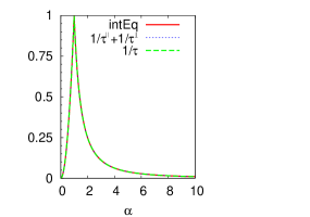
Remarkably, the AMR calculated from the distribution functions of Eqs. (III.3.2) or (III.3.1) and of Eq. (III.3.2), i.e. the exact and the two approximative results, comes out to be the same

$$\mbox{AMR}=\alpha^{2}\,,\ |\alpha|<1\qquad\mbox{AMR}=\frac{1}{\alpha^{2}}\,,\ |\alpha|>1\,.$$ (50)

Plot of this function is shown in Fig. 2(b).

For the two-band Rashba model with small $\lambda$, we thus conclude that the discrepancy between the exact and approximative approaches remains only on the level of the complete non-equilibrium distributions (in the higher order terms that do not contribute to the current). We speculate that the equal results for AMR were not obtained by coincidence but because the $\lambda\to 0$ system has a higher symmetry than the single-band model which is chiral. These symmetries are briefly commented in Appendix .4.

IV Discussion and conclusion

Let us start this discussion section with a remark on results shown in Fig. 2(a). The AMR takes on a singular value of $1$ at $\alpha=1$ in all three approaches. This reflects the $(1-\alpha^{2})^{-1}$ divergences of all non-equilibrium distribution functions (see Eq. (III.2) for example). The origin of this divergence is as follows: the scattering operator $\hat{V}$ in Eq. (10) with $\alpha=1$ can annihilate one particular state $|\vec{k}+\rangle$ on the Fermi surface, as seen from Eq. (54) and the spin textures in Fig. 1. The state has its spin aligned parallel to the moment of the magnetic impurities, i.e., along the $\hat{x}$-axis. For the Rashba model this implies that the $\vec{k}$-vector of this state is parallel to the $\hat{y}$-axis, more precisely $\phi=-\pi/2$. Within the $1/\tau$ approach, the fact that $(\alpha+\sigma_{x})|\vec{k}+\rangle=0$ then implies that this state has an infinite (transport) relaxation time as dictated by Eqs. (52) and (56) of the Appendix. Consequent calculation focusing also on other states $|\vec{k}\rangle$ contributing to the current shows that this singularity is strong enough to produce $\sigma_{yy}\to\infty$ when $|\alpha|\to 1$.

The current (and AMR) calculated for $|\alpha|$ close to 1 are clearly inconsistent with the linear-response basis of our theory approach (incorporated in Eq. (3)) and are therefore not physically relevant. On the other hand, the impurity operator (10) is idealised compared to realistic systems where the electric and magnetic part of $\hat{V}$ will depend at least slightly differently on $\vec{k}$. This modification suffices to remove the singularity in conductivity.

Pointing our attention more towards experiments, let us now discuss the relevance of the Rashba model with dilute charged magnetic scatterers. Our original motivation comes from the study of the diluted magnetic semiconductorJungwirth et al. (2006) (Ga,Mn)As. Mn atoms, when substituting for Ga, introduce both the magnetic moments and holes to the material. The former via its $d$-electrons and the latter because their valence number is one less than that of Ga. An ’electro-magnetic scatterer’ model as defined by Eq. (10) is therefore relevant to describe the Mn atoms which constitute by far the most frequent source of scattering in (Ga,Mn)As. Indeed, it is possible to qualitatively explain trends for AMR in (Ga,Mn)As based on this model of scattering and by neglecting the exchange splitting of the (Ga,Mn)As spin-orbit coupled valence band.Rushforth et al. (2007, 2008)

The Rashba model employed in this article provides arguably the simplest unpolarized spin-orbit coupled band structure in which the anisotropic scatterer mechanism fully determines the AMR. The other two mechanisms, which are the anisotropy of the group velocity and the anisotropy of wavefunctions of the spin-split spin-orbit-coupled valence band and which only quantitatively modify the calculated AMR in (Ga,Mn)As, are completely absent in this model. The simplicity of the present model relies mostly in that it is 2D and it considers two rotationally-symmetric rather than six warped bands of (Ga,Mn)As. The integral equation approach can be straightforwardly extended to (Ga,Mn)As or other three-dimensional systems with more ($n>2$) bands. However, the calculational complexity will be considerably higher; the two functions $a_{\pm}(\phi)$ of one variable will be replaced by $n$ functions of two variables (two angles parametrizing the Fermi surface in three dimensions).

Turning attention towards possible experiments, the calculations presented in this article are most relevant to asymmetric $n$-type heterostructures doped with magnetic donors.Mašek et al. (2007) By changing the Fermi level via doping, the effective strength $\alpha$ of the electric part of the scatterer should change because the scattering amplitudes depend on the Fermi wavevector which is a typical measure for involved momentum transfers.Rushforth et al. (2008) Consequently, by polarizing the magnetic moments in-plane, the AMR defined in Eq. (19) should be measurable and follow predictions shown in Fig. 2(a).

An alternative to doping by magnetic donors is to use an $n$-type heterostructure co-doped with magnetic impurities. Experimental study of a III-V or II-VI heterostructure with dilute Mn doping and heavy remote $n$-doping could be revealing. Depending on the magnetic impurity character (either acceptor or neutral), by varying the Fermi level, we could again effectively change $\alpha$ and/or interpolate between the single-band case ($\epsilon_{F}=0$) and the two-band case ($\epsilon_{F}\gg\lambda k_{F}$). The challenge in this experiment would be to keep the scattering on Mn the dominant (or at least strong) mechanism of relaxation.

Rather than these experimental suggestions, however, the main message of this paper should be of theoretical character. We have presented a framework to calculate exactly the conductivity in anisotropic systems within the semiclassical linear-response theory. This procedure was demonstrated on three simple and analytically solvable models. We found that in some special cases of high symmetry the previously employed approximate approaches may yield the same AMR as our exact theory. In general, however, only the exact non-equilibrium solution to Boltzmann equation of the form of an integral equation over the whole Fermi surface, rather than of effective scattering rates at each individual $\vec{k}$-point individually, provides a reliable account of the anisotropic transport.

APPENDIX

.1 Scattering rates

We evaluate the scattering rates using the Fermi golden rule. Probability $w_{fi}$ of transition between states $|i\rangle$ and $|f\rangle$, induced by a perturbation described by time-independent operator $\hat{V}$, equals

$$w_{fi}=\frac{2\pi}{\hbar}|\langle f|\hat{V}|i\rangle|^{2}\delta\big{(}\epsilon_{f}-\epsilon_{i}\big{)}\,,$$ (51)

where $\epsilon_{f/i}$ is the energy of the final/initial state.

Considering many scatterers described by the operator $\hat{V}$ distributed randomly with areal density $n_{i}$, the scattering rate per unit reciprocal space between the $\vec{k}$– and $\vec{k}^{\prime}$–state equals

$$w(\vec{k},\vec{k}^{\prime})=\frac{2\pi}{\hbar}n_{i}V_{0}^{2}|\langle\vec{k}^{\prime}|\hat{V}/V_{0}|\vec{k}\rangle|^{2}\delta\big{(}\epsilon_{\vec{k}}-\epsilon_{\vec{k}^{\prime}}\big{)}$$ (52)

within the lowest order of the Born approximation; contrary to the case of the anomalous Hall effectSinitsyn (2008); Kovalev et al. (2008), this order of the Born approximation is sufficient for the calculation of the AMR. Note that the dimension of the scatterer strength $V_{0}$ is J$\,\mbox{m}^{2}$, making $\hat{V}/V_{0}$ dimensionless in the Fourier space.

Finally, assuming isotropic parabolic dispersion $\epsilon_{\vec{k}}=\hbar^{2}k^{2}/2m$, the density of states equals $m/(h\hbar)$ per spin, so that

$$w(\phi,\phi^{\prime}) = \displaystyle\frac{1}{(2\pi)^{2}}\int_{0}^{\infty}k^{\prime}\,dk^{\prime}w(\vec{k},\vec{k}^{\prime})=$$

$$\hskip-56.9055pt=\frac{2\pi}{\hbar}n_{i}V_{0}^{2}\frac{m}{(2\pi\hbar)^{2}}|\langle\vec{k}^{\prime}|\hat{V}/V_{0}|\vec{k}\rangle|^{2}\equiv K|\langle\vec{k}^{\prime}|\hat{V}/V_{0}|\vec{k}\rangle|^{2}\,.$$

This is the definition of the dimensionful constant $K$ used in Eq. (11) and later on. Its value determines the absolute value of conductivity but it cancels out in the definition of the AMR, see Eq. (19).

.2 Scattering matrix elements

We calculate the matrix elements of the scattering operator $\hat{V}$ in Eq. (10) with respect to the basis

$$|\vec{k}\pm\rangle=\frac{1}{\sqrt{2}}\left(\begin{array}[]{c}1\\ \mp ie^{i\phi}\end{array}\right)\frac{1}{\sqrt{A}}e^{i\vec{k}\cdot\vec{r}}$$ (54)

where $\vec{k}=k(\cos\phi,\sin\phi)$ and $A$ is the system area. Vectors $|\vec{k}+\rangle$ and $|\vec{k}-\rangle$ are the eigenstates of Hamiltonian (9) with eigenvalues $\hbar^{2}k^{2}/2m-\lambda|\vec{k}|$ and $\hbar^{2}k^{2}/2m+\lambda|\vec{k}|$; their (expectation value of) spin $\vec{\sigma}=(\sigma_{x},\sigma_{y})$ is illustrated in Fig. 1. The scattering operator $\hat{V}$ in Eq. (10) is expressed in the basis of plane waves times spin up and spin down states. It does not depend on $\vec{k}$, $\vec{k}^{\prime}$ so that it corresponds to short-range impurities ($\delta$-scatterers). For $a\to\infty$, this would be a non-magnetic charged impurity of strength $aV_{0}$, and for $a=0$ it is a purely magnetic impurity of strength $V_{0}$.

Owing to the $\delta$-scatterer character of $\hat{V}$, the matrix elements of $\hat{V}/V_{0}$ in the basis (54) depend on $\vec{k}$ only through $\phi$ and not through $k=|\vec{k}|$. We take $k=k^{\prime}$ and get

$$\!\!\langle\vec{k}^{\prime}{+}|\alpha+\sigma_{x}|\vec{k}+\rangle = \frac{1}{2}\big{[}-ie^{i\phi}+ie^{-i\phi^{\prime}}+\alpha(1+e^{i(\phi-\phi^{\prime})})\big{]}$$

$$\langle\vec{k}^{\prime}{-}|\alpha+\sigma_{x}|\vec{k}-\rangle = \frac{1}{2}\big{[}ie^{i\phi}-ie^{-i\phi^{\prime}}+\alpha(1+e^{i(\phi-\phi^{\prime})})\big{]}$$

$$\langle\vec{k}^{\prime}{+}|\alpha+\sigma_{x}|\vec{k}-\rangle = \frac{1}{2}\big{[}ie^{i\phi}+ie^{-i\phi^{\prime}}+\alpha(1-e^{i(\phi-\phi^{\prime})})\big{]}$$

$$= \overline{\langle\vec{k}{-}|\alpha+\sigma_{x}|\vec{k}^{\prime}+\rangle}\,.$$

Taking the absolute values squared leads using Eq. (.1) to Eq. (40), to Eq. (21) (the ’++’ element), and to Eq. (11) (’++’ element with $\alpha=0$).

.3 The $1/\tau$ approach

Non-equilibrium distribution function in an isotropic ($\epsilon_{\vec{k}}=\epsilon_{k}$, and isotropic scatterer) two-band system can be shown to be

$$f_{\pm}(\phi,\theta)=f_{\pm}(\phi-\theta)=f_{0}-e\vec{v}_{\pm}\cdot\vec{\cal E}\left(-\frac{\partial f_{0\pm}}{\partial\epsilon}\right)\tau_{\pm}\,,$$ (55)

where the relaxation times for $+$ and $-$ bands may depend on $\vec{k}$ only through energy $\epsilon_{k}$. This fact, that for fixed energy the relaxation time as defined in Eq. (1) is constant, is a direct consequence of the scatterer isotropy $w(\vec{k},\vec{k}^{\prime})=w(\vartheta_{\vec{k}\vec{k}^{\prime}})$. For clarity, we stress that in an $n$–band system there are the total of $n^{2}$ scattering rates between pairs of bands,

$$\frac{1}{\tau_{ba}}=\int\frac{d^{2}k^{\prime}}{(2\pi)^{2}}w_{ba}(\vec{k},\vec{k}^{\prime})\left[1-\frac{|\vec{v}_{b}(\vec{k}^{\prime})|}{|\vec{v}_{a}(\vec{k})|}\cos\vartheta_{\vec{v}\vec{v}^{\prime}}\right]\,,$$ (56)

that combine into $n$ scattering times $\tau_{a}$, one for each band, according to the Matthiessen’s ruleAshcroft and Mermin (1976)

$$\frac{1}{\tau_{a}}=\sum_{b}\frac{1}{\tau_{ba}}\,.$$ (57)

We note that $\vartheta_{\vec{v}\vec{v}^{\prime}}$ measures the angle between $\vec{v}_{b}(\vec{k}^{\prime})$ and $\vec{v}_{a}(\vec{k})$ but given the isotropy of the band structure, $\vec{v}(\vec{k})$ and $\vec{k}$ are parallel so that $\vartheta_{\vec{v}\vec{v}^{\prime}}=\vartheta_{\vec{k}\vec{k}^{\prime}}$. Equation (1) is a single-band variant of Eq. (56) for isotropic systems where $v$ drops out.

In the $1/\tau$ approach, we simply evaluate Eq. (56) for $w(\vec{k},\vec{k}^{\prime})\not=w(\vartheta_{\vec{k}\vec{k}^{\prime}})$ and obtain $\vec{k}$–dependent $1/\tau$. This is then inserted into the distribution function (55), losing thereby its property $f_{\pm}(\phi,\theta)=f_{\pm}(\phi-\theta)$.

For the Rashba model with $\lambda\to 0$ we get using Eq. (.1) and Appendix .2 the following

$$\begin{array}[]{rcl}\tau^{-1}_{(++/--)}(\phi)\!\!&=&\!\!K\pi\big{(}(+/-)2\alpha\sin\phi+3-2\sin^{2}\phi+\alpha^{2}\big{)}\\ \tau^{-1}_{(+-/-+)}(\phi)\!\!&=&\!\!K\pi\big{(}(-/+)6\alpha\sin\phi+1+2\sin^{2}\phi+3\alpha^{2}\big{)}\,.\end{array}$$ (58)

The scattering rates in the two-band model are thus as simple as

$$\frac{1}{\tau_{\pm}(\phi)}=\frac{1}{\tau_{+\pm}(\phi)}+\frac{1}{\tau_{-\pm}(\phi)}=\frac{1/(4\pi K)}{1\pm 2\alpha\sin\phi+\alpha^{2}}\,.$$ (59)

This result, plugged into Eq. (55), produces the non-equilibrium distribution function (III.3.2) within the $1/\tau$ approach.

The relaxation time for the single band model is simply $1/\tau(\phi)=1/\tau_{++}(\phi)$. Setting here $\alpha=0$ leads via Eq. (55) to Eq. (III.1).

.4 The $1/\tau^{\parallel}\,\&\,1/\tau^{\perp}$ approach

The prescription for the non-equilibrium distribution function suggested by Schliemann and LossSchliemann and Loss (2003) can be summarized as follows: (a) evaluate the ’standard’ formulae (57,56) and denote the result as $1/\tau^{\parallel}_{a}(\phi)$; (b) calculate $1/\tau^{\perp}_{a}(\phi)$ using formulae identical to Eqs. (56,57) save the replacement of the bracket in Eq. (56) by $|v_{b}(\vec{k}^{\prime})|/|v_{a}(\vec{k})|\,\sin\vartheta_{\vec{v}\vec{v}^{\prime}})$; (c) write down the distribution function as

$$f_{\pm}(\phi,\theta) = f_{0}-e|\vec{v}_{\pm}|\,|\vec{\cal E}|(-\partial_{\epsilon}f_{0\pm})\times$$

$$\hskip-56.9055pt\tau_{\pm}^{\parallel}\!\left[\cos(\phi-\theta)\frac{(\tau_{\pm}^{\perp})^{2}}{(\tau_{\pm}^{\parallel})^{2}+(\tau_{\pm}^{\perp})^{2}}\!+\!\sin(\phi-\theta)\frac{\tau_{\pm}^{\perp}\tau_{\pm}^{\parallel}}{(\tau_{\pm}^{\parallel})^{2}+(\tau_{\pm}^{\perp})^{2}}\!\right]\,.$$

Several remarks are in order. (i) Whenever $1/\tau_{\pm}^{\perp}$ vanishes, Eq. (.4) simplifies to Eq. (55) of the $1/\tau$ approach. (ii) This $1/\tau^{\parallel}\,\&\,1/\tau^{\perp}$ approach is suitable for the description of isotropic scatterers (the amplitude depends only on the angle between $\vec{k}$ and $\vec{k}^{\prime}$, the incoming and outgoing wave) which however may exhibit an asymmetry (or better chirality), i.e. scatter more clockwise than counterclockwise — such as it is the case with skew scattering in the anomalous Hall effect. (iii) Contrary to the statement of Ref. Schliemann and Loss, 2003, the distribution function (.4) is not the exact solution to Eq. (III.3) for a general anisotropic system. The derivation of Eq. (.4) presented in Ref. Schliemann and Loss, 2003 is only valid if the expressions

$$\frac{\tau_{a}^{\parallel}}{1+\big{(}\tau_{a}^{\parallel}/\tau_{a}^{\perp}\big{)}^{2}}\,,\quad\frac{\tau_{a}^{\perp}}{1+\big{(}\tau_{a}^{\perp}/\tau_{a}^{\parallel}\big{)}^{2}}\,,$$

given by Eq. (27,28) of that reference are constant for each band (i.e. $\phi$–independent in our case). The most general distribution function this approach can therefore correctly capture must have the form

$$f(\phi,\theta)-f_{0}=C_{1}\cos(\phi-\theta)+C_{2}\sin(\phi-\theta)$$

while as the examples in Section II show, the non-equilibrium distribution can have finer details than those of period $2\pi$ in the angular variable $\phi$ (and these details, when completely neglected, may even lead to wrong values of the constants $C_{1}$, $C_{2}$ above). This original neglect of Ref. Schliemann and Loss, 2003 was later corrected by one of its authorsTrushin and Schliemann (2007) in the context of the specific Hamiltonian considered.Schliemann and Loss (2003) However, a general procedure for exact solution of the Boltzmann equation was not given.

In our specific model, as described by the scattering matrix elements of Appendix .2, we get

$$\begin{array}[]{rcl}[\tau^{\perp}_{(++/--)}(\phi)]^{-1}&=&K\pi\cos\phi\big{(}(+/-)\alpha+\sin\phi\big{)}\\[0.0pt] [\tau^{\perp}_{(+-/-+)}(\phi)]^{-1}&=&K\pi\cos\phi\big{(}(+/-)\alpha-\sin\phi\big{)}\,.\end{array}$$ (61)

For the two-band model,

$$\frac{1}{\tau^{\perp}_{+}(\phi)}=\frac{1}{\tau^{\perp}_{++}(\phi)}+\frac{1}{\tau^{\perp}_{-+}(\phi)}=0\,,\qquad\frac{1}{\tau^{\perp}_{-}(\phi)}=0\,,$$ (62)

so that the $1/\tau^{\parallel}\,\&\,1/\tau^{\perp}$ approach reduces to the $1/\tau$ approach in line with the comment after Eq. (.4). The single-band case, however, has a finite $\tau^{\perp}\equiv\tau_{++}^{\perp}$ so that the two approaches give different results. This is not surprising, since each Rashba band has a chiral spin texture but both of them together form a non-chiral pair, provided they have both the same Fermi $k$ (as it happens for $\lambda\to 0$), see Fig. 1. The asymmetry of scattering expressed by $1/\tau^{\perp}$ thus vanishes in our two-band model.

To obtain the non-equilibrium distribution (III.1) within the $1/\tau^{\parallel}\,\&\,1/\tau^{\perp}$ approach, we have to take $1/\tau^{\parallel}_{++}$ of Eq. (58), $1/\tau^{\perp}_{++}$ of Eq. (61), insert them into Eq. (.4) and expand $\cos(\phi-\theta)$, $\sin(\phi-\theta)$ in terms of $\cos\theta$ and $\sin\theta$.

.5 Partitioning method

The actual infinite system of linear equations for variables $a_{0},a_{c1},a_{s1},\ldots$ appropriate for the single-band model assumes a structure suitable for partitioning if we perform the coordinate transformation $\tilde{\varphi}=\pi/2-\phi$. We will now solve the integral equation (7) using this coordinate (and use $\tilde{\varphi}$ throughout Appendices .5 and .6) and transform the result back before we use it in Eq. (22).

The equation to be solved is now

$$\bar{w}(\tilde{\varphi})\tilde{a}(\tilde{\varphi})-\int d\tilde{\varphi}^{\prime}w(\tilde{\varphi},\tilde{\varphi}^{\prime})\tilde{a}(\tilde{\varphi}^{\prime})=\sin\tilde{\varphi}$$ (63)

with

$$w(\tilde{\varphi},\tilde{\varphi}^{\prime}) = \textstyle\frac{1}{2}K\big{[}1+\cos(\tilde{\varphi}+\tilde{\varphi}^{\prime})+\alpha^{2}\big{(}1+\cos(\tilde{\varphi}-\tilde{\varphi}^{\prime})\big{)}]+$$

$$+\alpha(\cos\tilde{\varphi}+\cos\tilde{\varphi}^{\prime})$$

$$\bar{w}(\tilde{\varphi}) = \pi K(1+\alpha^{2}+2\alpha\cos\tilde{\varphi})\,.$$

Inserting

$$\tilde{a}(\tilde{\varphi})=\tilde{a}_{0}+\tilde{a}_{c1}\cos\tilde{\varphi}+\ldots+\tilde{a}_{s1}\sin\tilde{\varphi}+\ldots$$

into Eq. (63), and comparing the coefficients at the constant, $\cos\tilde{\varphi}$, $\sin\tilde{\varphi}$, $\cos 2\tilde{\varphi}$, $\cos 3\tilde{\varphi}$, $\ldots$, $\sin 2\tilde{\varphi}$, $\ldots$ terms, we obtain the following infinite system of linear equations for $\tilde{a}_{0},\tilde{a}_{c1},\tilde{a}_{s1},\tilde{a}_{c2},\tilde{a}_{c3},\ldots,\tilde{a}_{s2},\tilde{a}_{s3},\ldots$ (in this order):

$$\hskip-11.38109pt\left(\begin{array}[]{ccc|cccc|cccc||c}*&*&*&0&0&0&\ldots&0&0&0&\ldots&*\\[0.0pt] *&*&*&\alpha&0&0&\ldots&0&0&0&\ldots&*\\[0.0pt] *&*&*&0&0&0&\ldots&\alpha&0&0&\ldots&*\\ \hline\cr 0&\alpha&0&\!1+\alpha^{2}\!\!\!&\alpha&0&\ldots&0&0&0&\ldots&0\\ 0&0&0&\alpha&\!\!\!1+\alpha^{2}\!\!\!&\alpha&&0&0&0&\ldots&0\\ 0&0&0&0&\alpha&\!\!\!1+\alpha^{2}\!\!\!&&0&0&0&\ldots&0\\ \vdots&&&\vdots&&&\ddots&\vdots&&&\vdots&\vdots\\ \hline\cr 0&0&\alpha&0&0&0&\!\ldots&1+\alpha^{2}&\alpha&0&\ldots&0\\[-5.69054pt] 0&0&0&0&0&0&\ldots&\alpha&\ddots&&\vdots&0\\ \vdots&&&&&&&&&&\vdots&\vdots\end{array}\right)$$ (64)

The double line separates the left and right-hand side of the equations. The twelve asterisks in the first three lines of the system (64) correspond to the $3\times 3$ system (22), and the value of these coefficients will be unimportant within this Appendix.

It is apparent that the system (64) is almost block-diagonal. The partitioning method takes advantage of this structure and aims at solving three independent systems corresponding to groups $\{\tilde{a}_{0},\tilde{a}_{c1},\tilde{a}_{s1}\}$, $\{\tilde{a}_{c2},\tilde{a}_{c3},\ldots\}$, and $\{\tilde{a}_{s2},\tilde{a}_{s3},\ldots\}$ of the original variables. The basic idea is to treat the only non-zero element of the off-diagonal block as a right-hand-side term. In explicite terms, we rewrite for example the fourth and fifth equations of the system (64)

$$[\alpha\tilde{a}_{c1}+(1+\alpha^{2})\tilde{a}_{c2}+\alpha\tilde{a}_{c3}]\cos 2\tilde{\varphi} = 0$$

$$[\alpha\tilde{a}_{c2}+(1+\alpha^{2})\tilde{a}_{c3}+\alpha\tilde{a}_{c4}]\cos 3\tilde{\varphi} = 0$$

as

$$(1+\alpha^{2})\tilde{a}_{c2}+\alpha\tilde{a}_{c3}\phantom{\alpha\tilde{a}_{c2}+}\ = -\alpha\tilde{a}_{c1}\equiv\Delta$$

$$\alpha\tilde{a}_{c2}+(1+\alpha^{2})\tilde{a}_{c3}+\alpha\tilde{a}_{c4} = 0\,.$$

The system of all ’cosine-term’ equations of the system (64) (starting with $\cos 2\tilde{\varphi}$) can now be solved as a function of $\Delta$. In other words, we are treating the central block of the matrix (64). The still-infinite system to be solved is

$$\left(\begin{array}[]{ccccc||c}1+\alpha^{2}&\alpha&0&0&\ldots&\Delta\\ \alpha&1+\alpha^{2}&\alpha&0&\ldots&0\\ 0&\alpha&1+\alpha^{2}&\alpha&\ldots&0\\ \vdots&&&\ddots&\vdots&\vdots\end{array}\right)\,.$$ (65)

For the purposes of solving later the $3\times 3$ system (22), we in fact need to know only a part of the solution, namely $\tilde{a}_{c2}$. To this end, linear algebra gives us a very quick answer. If we denote by $D$ the determinant of the infinite matrix left from the double line in (65), and by $D_{n}$ the determinant of the analogous $n\times n$ matrix, then if the system (65) were finite,

$$\tilde{a}_{c2}=\frac{\Delta D_{n-1}}{D_{n}}\,,$$

where the numerator equals the determinant of the $n\times n$ matrix left from the double line of (65) with first column replaced by the column right from the double line. Considering $n\to\infty$, we immediatelly (after transformation $a_{c2}=-\tilde{a}_{c2}$) get $\tilde{a}_{c2}=-\Delta$ as given in the first line of Eq. (23). This answer is, however, not completely correct.

The caveat of this procedure is that we should have been careful about taking the limit $D=\lim_{n\to\infty}D_{n}$. It turns out that the limit is finite only for $|\alpha|<1$ and then $D=1/(1-\alpha^{2})$ so that only in this case $\lim D_{n-1}/D_{n}=(\lim D_{n-1})/(\lim D_{n})$ which is obviously equal to one. The determinant $D$ is infinite for $|\alpha|>1$ and only $\lim_{n\to\infty}D_{n-1}/D_{n}$ remains finite, namely equal to $1/\alpha^{2}$ as one can readily see from the explicit formula

$$D_{n}=1+\alpha^{2}+\alpha^{4}+\ldots+\alpha^{2n}\,.$$

In conclusion, we find

$$\tilde{a}_{c2}=\left\{\begin{array}[]{ll}\Delta&\mbox{ for }|\alpha|<1\\ \Delta/\alpha^{2}&\mbox{ for }|\alpha|>1\end{array}\right.$$ (66)

and the transformation back from $\tilde{\varphi}$ to $\phi$ implies $a_{c2}=-\tilde{a}_{c2}$ and $\tilde{a}_{c1}=a_{s1}$.

Literally the same procedure works for the ’sine-term’ equations of the system (64), i.e. the lower-right block. The only difference is now that $\Delta=-a\tilde{a}_{s1}$ and we use $a_{s2}=\tilde{a}_{s2}$, $\tilde{a}_{s1}=a_{c1}$. These two results, $a_{c2},a_{s2}$ with the corresponding definitions of $\Delta$ are summarized as Eq. (23).

The key feature needed for this partitioning method is that $\Delta$ is a function only of $\tilde{a}_{c1}$ ($\tilde{a}_{s1}$) and not of higher-order coefficients like $\tilde{a}_{c3}$. In this way, the $3\times 3$ system of equations (22) becomes closed after $a_{c2}$ and $a_{s2}$ have been inserted.

Finally, we stress, that if the coupling between the three subsystems had been neglected from the very beginning — this amounts to setting to zero the four elements in the off-diagonal blocks in the system (64) — the solution of the $3\times 3$ subsystem represented by the asterisks would have been different. In this way, even though $\cos 2\phi$ and other higher terms do not contribute to the current calculated from the non-equilibrium distribution (5), their complete neglect from the beginning may produce wrong coefficients in the $\cos\phi$ and $\sin\phi$ terms.

.6 Partitioning method – two bands

In the case of two bands, we obtain two infinite systems of linear equations identical to the system (64), one for variables with ’+’ index, another for those with ’$-$’ index, see Eq. (41). Although the two systems are now coupled, the direct coupling exists only via variables $\tilde{a}_{0\pm}$, $\tilde{a}_{c1\pm}$, $\tilde{a}_{s1\pm}$ corresponding to the upper left block. The partitioning method can therefore be independently carried out in the ’$+$’ and ’$-$’ sector.

For all four infinite subsystems, of which the system (65) is one, we obtain the almost the same result

$$\tilde{a}_{cn+},\,\tilde{a}_{sn+}=\left\{\begin{array}[]{ll}\Delta(-\alpha)^{n-2}&\mbox{ for }|\alpha|<1\\ \Delta/(-\alpha)^{n}&\mbox{ for }|\alpha|>1\,,\end{array}\right.$$ (67)

for $n\geq 2$ and with appropriate definition of $\Delta$ for each subsystem, while $\tilde{a}_{cn-},\tilde{a}_{sn-}$ obey Eq. (67) with $-a$ replaced by $a$. All coefficients in the series (41) are thus non-zero. Nevertheless, Eq. (41) can still be summed up using

$$\sum_{n=0}^{\infty}(-\alpha)^{n}\cos n\tilde{\varphi}=\frac{1+\alpha\cos\tilde{\varphi}}{1+\alpha^{2}+2\alpha\cos\tilde{\varphi}}$$

and a similar formula for sines. We now transform back from $\tilde{\varphi}$ to $\phi$, use $\Delta=\mp\alpha\tilde{a}_{c1\pm}$ for the cosine $\pm$ parts of Eq. (41) and $\Delta=\mp\alpha\tilde{a}_{s1\pm}$ for its sine parts, transform back $\tilde{a}_{c1\pm}=a_{s1\pm}$, $\tilde{a}_{s1\pm}=a_{c1\pm}$ and finally get

$$\begin{array}[]{rcl}a_{+}(\phi)&=&a_{0+}+\\ &&\hskip-22.76228pt\displaystyle a_{c1+}\frac{\cos\phi}{1+\alpha^{2}+2\alpha\sin\phi}+a_{s1+}\frac{\alpha+\sin\phi}{1+\alpha^{2}+2\alpha\sin\phi}\\ a_{-}(\phi)&=&a_{0+}+\\ &&\hskip-22.76228pt\displaystyle a_{c1-}\frac{\cos\phi}{1+\alpha^{2}-2\alpha\sin\phi}+a_{s1-}\frac{-\alpha+\sin\phi}{1+\alpha^{2}-2\alpha\sin\phi}\,.\end{array}$$ (68)

Plugging the values of $a_{0+},a_{c1+},a_{s1+}$ from Eq. (45) into Eq. (68), repeating an analogous procedure for the $b$’s in Eq. (39) and inserting the results into Eq. (29), we arrive at Eq. (III.3.2).

.7 Boltzmann equation in general 2D anisotropic systems

Results of Section II were derived for a special class of 2D systems where the band structure remains isotropic and the anisotropy is only introduced through the scatterer and the scattering rate $w(\vec{k},\vec{k}^{\prime})$.

The results of Eqs. (7,8) for single-band or of Eqs. (34,39) for two-band system have to be slightly modified for anisotropic 2D band structure. The wavevectors $\vec{k},\vec{k}^{\prime}$ of Eq. (3) or Eqs. (III.3) will still be bound to the Fermi level $\epsilon_{F}$ but their magnitude now depends on $\phi$. That is, we have $k=k(\phi)$ and $\vec{k}=k\hat{n}=k(\cos\phi,\sin\phi)$. We also tacitly assume that in each band and for each $\hat{n}$ there is only one solution $k$ to $\epsilon_{k\hat{n}}=\epsilon_{F}$. The calculation of $w(\phi,\phi^{\prime})$, compared to what is done in Appendix .1, becomes

$$w(\phi,\phi^{\prime}) = \displaystyle\frac{1}{(2\pi)^{2}}\int_{0}^{\infty}k^{\prime}\,dk^{\prime}w(\vec{k},\vec{k}^{\prime})=$$

$$= \frac{2\pi}{\hbar}n_{i}V_{0}^{2}\left|\nabla_{\vec{k}^{\prime}}\epsilon_{\vec{k}^{\prime}}\cdot\vec{k}^{\prime}/{k^{\prime}}^{2}\right|^{-1}\!|\langle\vec{k}^{\prime}|\hat{V}/V_{0}|\vec{k}\rangle|^{2}\,.$$

The last expression should be understood as a function of $\phi$, $\phi^{\prime}$ only; the derivative and $\vec{k},\vec{k}^{\prime}$ are to be taken at the Fermi level, so that e.g. $\vec{k}^{\prime}=k^{\prime}(\cos\phi^{\prime},\sin\phi^{\prime})$ and $\epsilon_{\vec{k}^{\prime}}=\epsilon_{F}$.

Further, the expression $\vec{\cal E}\cdot\vec{v}(\vec{k})$ in Eq. (3) is no longer simply ${\cal E}v\cos(\theta-\phi)$. First of all, $v=v(\phi)$ and moreover $\vec{v}$ need not be parallel with $\vec{k}$. Formally, we could replace $\theta-\phi$ in Eq. (6) by $\theta-\xi(\phi)$ with $\xi$ defined by $\vec{v}(\vec{k})=(\cos\xi,\sin\xi)v(\phi)$. Single-band equations (7,8) should be replaced by

$$\hskip-14.22636pt\cos\xi(\phi) = \bar{w}(\phi)\,a(\phi)-\int d\phi^{\prime}\frac{v(\phi^{\prime})}{v(\phi)}w(\phi,\phi^{\prime})a(\phi^{\prime})$$ (70)

$$\hskip-14.22636pt\sin\xi(\phi) = \bar{w}(\phi)\,b(\phi)-\int d\phi^{\prime}\frac{v(\phi^{\prime})}{v(\phi)}w(\phi,\phi^{\prime})b(\phi^{\prime})\,.$$ (71)

These two equations for $a(\phi)$ and $b(\phi)$ are still completely decoupled. With some luck, $\cos\xi(\phi)$ can be reasonably expanded in terms of cosines and sines of $\phi$ and higher multiples of $\phi$ but the $v(\phi)$ and $v(\phi^{\prime})$ terms will most likely make an analytical solution of Eq. (70) impossible for realistic anisotropic Fermi surfaces. The solution is, however, not difficult to obtain by numerical means. After discretization of the angular variable $\phi$ into $n$ steps, Eq. (70) constitutes an $n\times n$ system of linear equations.

Once $a(\phi),b(\phi)$ are known, the non-equilibrium distribution function is readily written as

$$f(\vec{k},\vec{\cal E})-f_{0} = f(\phi,\theta)-f_{0}=$$

$$-e{\cal E}v(\phi)(-\partial_{\epsilon}f_{0})\big{[}a(\phi)\cos\theta+b(\phi)\sin\theta\big{]}\,.$$

Note that the spectral function $-\partial_{\epsilon}f_{0}=\delta(\epsilon_{F}-\epsilon_{\vec{k}})$ depends now both on $k$ and $\phi$.

A rather straightforward generalization of Eq. (.7) and the appropriate pair of integral equations (70,71) to multiband systems is possible. For instance, the analogy of the two coupled Eqs. (34) for anisotropic band structure reads

$$\cos\xi_{+}(\phi) = \bar{w}_{+}(\phi)\,a_{+}(\phi)-\int d\phi^{\prime}\times$$

$$\displaystyle\hskip-56.9055pt\times\left[\frac{v_{+}(\phi^{\prime})}{v_{+}(\phi)}w_{++}(\phi,\phi^{\prime})a_{+}(\phi^{\prime})+\frac{v_{-}(\phi^{\prime})}{v_{+}(\phi)}w_{+-}(\phi,\phi^{\prime})a_{-}(\phi^{\prime})\right]$$

$$\cos\xi_{-}(\phi) = \bar{w}_{-}(\phi)\,a_{-}(\phi)-\int d\phi^{\prime}\times$$

$$\displaystyle\hskip-56.9055pt\times\left[\frac{v_{-}(\phi^{\prime})}{v_{-}(\phi)}w_{--}(\phi,\phi^{\prime})a_{-}(\phi^{\prime})+\frac{v_{+}(\phi^{\prime})}{v_{-}(\phi)}w_{-+}(\phi,\phi^{\prime})a_{+}(\phi^{\prime})\right]$$

where $\vec{v}_{\pm}=(\cos\xi_{\pm},\sin\xi_{\pm})v_{\pm}(\phi)$ are the Fermi velocities of the two bands and the four quantities $w_{\pm\pm}(\phi,\phi^{\prime})$ have to be calculated in the spirit of Eq. (.7).

References

- Thomson (1857) W. Thomson, Proc. Roy. Soc. London 8, 546 (1857).
- Döring (1938) W. Döring, Ann. Phys. (Leipzig) 424, 259 (1938).
- Jaoul et al. (1977) O. Jaoul, I. A. Campbell, and A. Fert, J. Magn. Magn. Mater. 5, 23 (1977).
- Zutic et al. (2004) I. Zutic, J. Fabian, and S. Das Sarma, Rev. Mod. Phys. 76, 323 (2004), eprint arXiv:cond-mat/0405528.
- Fabian et al. (2007) J. Fabian, A. Matos-Abiague, C. Ertler, P. Stano, and I. Zutic, Acta Physica Slovaca 57, 565 (2007), eprint arXiv:0711.1461.
- Smit (1951) J. Smit, Physica 17, 612 (1951).
- Berger (1964) L. Berger, Physica 30, 1141 (1964).
- McGuire and Potter (1975) T. McGuire and R. Potter, IEEE Trans. Magn. 11, 1018 (1975).
- Banhart and Ebert (1995) J. Banhart and H. Ebert, Europhys. Lett. 32, 517 (1995).
- Rushforth et al. (2008) A. W. Rushforth, K. Výborný, C. S. King, K. W. Edmonds, R. P. Campion, C. T. Foxon, J. Wunderlich, A. C. Irvine, V. Novák, K. Olejník, et al., J. Mag. Magn. Mater. (2008), eprint arXiv:0712.2581.
- Rushforth et al. (2007) A. W. Rushforth, K. Výborný, C. S. King, K. W. Edmonds, R. P. Campion, C. T. Foxon, J. Wunderlich, A. C. Irvine, P. Vašek, V. Novák, et al., Phys. Rev. Lett. 99, 147207 (2007), eprint arXiv:cond-mat/0702357.
- Ashcroft and Mermin (1976) N. W. Ashcroft and N. D. Mermin, Solid State Physics (Saunders College Publishing, Philadelphia, 1976).
- Schliemann and Loss (2003) J. Schliemann and D. Loss, Phys. Rev. B 68, 165311 (2003).
- Sinitsyn et al. (2007) N. A. Sinitsyn, A. H. MacDonald, T. Jungwirth, V. K. Dugaev, and J. Sinova, Phys. Rev. B 75, 045315 (2007), eprint arXiv:cond-mat/0608682.
- Sinitsyn (2008) N. A. Sinitsyn, J. Phys.: Condens. Matter 20, 023201 (2008), eprint arXiv:0712.0183.
-
(16)
(URL)
http://en.wikipedia.org/wiki/
Fredholm_integral_equation - Trushin and Schliemann (2007) M. Trushin and J. Schliemann, Phys. Rev. B 75, 155323 (2007), eprint arXiv:cond-mat/0611328.
- Jungwirth et al. (2006) T. Jungwirth, J. Sinova, J. Mašek, J. Kučera, and A. H. MacDonald, Rev. Mod. Phys. 78, 809 (2006), eprint arXiv:cond-mat/0603380.
- Mašek et al. (2007) J. Mašek, J. Kudrnovský, F. Máca, B. L. Gallagher, R. P. Campion, D. H. Gregory, and T. Jungwirth, Phys. Rev. Lett. 98, 067202 (2007), eprint arXiv:cond-mat/0609184.
- Kovalev et al. (2008) A. A. Kovalev, K. Výborný, and J. Sinova, Phys. Rev. B 78, 041305 (2008), eprint arXiv:0803.1226.