Renormalization group evolution of neutrino mixing parameters near $\theta_{13}=0$ and models with vanishing $\theta_{13}$ at the high scale

Abstract

Renormalization group (RG) evolution of the neutrino mass matrix may take the value of the mixing angle $\theta_{13}$ very close to zero, or make it vanish. On the other hand, starting from $\theta_{13}=0$ at the high scale it may be possible to generate a non-zero $\theta_{13}$ radiatively. In the most general scenario with non-vanishing CP violating Dirac and Majorana phases, we explore the evolution in the vicinity of $\theta_{13}=0$, in terms of its structure in the complex ${\cal U}_{e3}$ plane. This allows us to explain the apparent singularity in the evolution of the Dirac CP phase $\delta$ at $\theta_{13}=0$. We also introduce a formalism for calculating the RG evolution of neutrino parameters that uses the Jarlskog invariant and naturally avoids this singular behaviour. We find that the parameters need to be extremely fine-tuned in order to get exactly vanishing $\theta_{13}$ during evolution. For the class of neutrino mass models with $\theta_{13}=0$ at the high scale, we calculate the extent to which RG evolution can generate a nonzero $\theta_{13}$, when the low energy effective theory is the standard model or its minimal supersymmetric extension. We find correlated constraints on $\theta_{13}$, the lightest neutrino mass $m_{0}$, the effective Majorana mass $m_{ee}$ measured in the neutrinoless double beta decay, and the supersymmetric parameter $\tan\beta$.

I Introduction

In the last decade, neutrino experiments have reached a stage where the basic structure of the neutrino masses and mixing is more or less clear. We know that the three neutrino flavors ($\nu_{\alpha},\alpha\in\{e,\mu,\tau\}$) mix to form three neutrino mass eigenstates ($\nu_{i},i\in\{1,2,3\}$), which are separated by $\Delta m^{2}_{ij}\equiv m_{i}^{2}-m_{j}^{2}$ where, $m_{i,j}$ denote mass eigenvalues with $i,j\in\{1,2,3\}$. The two sets of eigenstates are connected through $\nu_{\alpha}=(U_{\rm PMNS})_{\alpha i}\nu_{i}$, where $U_{\rm PMNS}$ is the Pontecorvo-Maki-Nakagawa-Sakata neutrino mixing matrix pontecorvo ; mns in the basis where the charged lepton mass matrix is assumed to be diagonal. This matrix is parametrized as

$$U_{\rm PMNS}=\left(\begin{array}[]{ccc}e^{i\chi_{1}}&0&0\\ 0&e^{i\chi_{2}}&0\\ 0&0&e^{i\chi_{3}}\\ \end{array}\right)\cdot{\cal U}\cdot\left(\begin{array}[]{ccc}e^{i\phi_{1}}&0&0\\ 0&e^{i\phi_{2}}&0\\ 0&0&1\\ \end{array}\right)\;,$$ (1)

where ${\cal U}$ is the matrix

$${\cal U}=\left(\begin{array}[]{ccc}c_{12}c_{13}&s_{12}c_{13}&s_{13}e^{-i\delta}\\ -s_{12}c_{23}-c_{12}s_{23}s_{13}e^{i\delta}&c_{12}c_{23}-s_{12}s_{23}s_{13}e^{i\delta}&s_{23}c_{13}\\ s_{12}s_{23}-c_{12}c_{23}s_{13}e^{i\delta}&-c_{12}s_{23}-s_{12}c_{23}s_{13}e^{i\delta}&c_{23}c_{13}\\ \end{array}\right)\;.$$ (2)

Here $c_{ij}$ and $s_{ij}$ are the cosines and sines respectively of the mixing angle $\theta_{ij}$, $\delta$ is the Dirac CP violating phase, $\phi_{i}$ are the Majorana phases, and $\chi_{i}$ are the so-called unphysical phases that do not play a role in the phenomenology of neutrino mixing, but whose values may be predictable within the context of specific models. The current best-fit values and 3$\sigma$ ranges for these parameters are summarized in Table 1. It is not known whether the neutrino mass ordering is normal ($m_{1}<m_{2}<m_{3}$) or inverted ($m_{3}<m_{1}<m_{2}$).

		Best fit		$3\sigma$ range
$\Delta m_{21}^{2}$ [$10^{-5}{\rm eV}^{2}$]		7.65		7.05 - 8.34
$|\Delta m_{31}^{2}|$ [$10^{-3}{\rm eV}^{2}$]		2.40		2.07 - 2.75
$\sin^{2}\theta_{12}$		0.304		0.25 - 0.37
$\sin^{2}\theta_{23}$		0.50		0.36 - 0.67
$\sin^{2}\theta_{13}$		0.01		$\leq$ 0.056

Table 1: The present best-fit values and 3$\sigma$ ranges of oscillation parameters Schwetz:2008er .

An intriguing situation with the neutrino mixing is that two of the mixing angles, $\theta_{12}$ and $\theta_{23}$, are definitely large, while the third angle $\theta_{13}$ is small and may even be zero. Such a situation is indicative of some kind of symmetry principle at work. Indeed, there is a whole class of models with $\theta_{13}\approx 0$ that are consistent with data albright . $\theta_{23}=\pi/4$ and $\theta_{13}=0$ are allowed by the current data and their origin has been traced to an exact $\mu-\tau$ exchange symmetry in the neutrino mass matrix mutau . Such symmetries can be realized by models based on the discrete non-abelian symmetry groups like $A_{4}$ a4 , $D_{4}$ d4 , $S_{3}$ s3 , $S_{4}$ s4 . Special cases of an exact $\mu-\tau$ symmetric matrix corresponding to a $L_{e}$ symmetry for normal ordering le , $L_{e}-L_{\mu}-L_{\tau}$ symmetry for inverted ordering le-lmu-ltau and $L_{\mu}-L_{\tau}$ symmetry for quasidegenerate neutrinos can give $\theta_{13}=0$ lmu-ltau . Any deviation from this value would indicate breaking of these symmetries. Models with discrete abelian symmetries can also make $\theta_{13}$ vanish low . Models involving certain texture zeroes in the neutrino Yukawa matrix or certain scaling relations between Majorana matrix elements can also predict zero or almost vanishing $\theta_{13}$ texture . SO(10) models with certain structures for Dirac mass matrices so10 , or those with a SO(3) symmetry can predict $\theta_{13}\lesssim 10^{-4}$ with a normal mass ordering so3 .

Most of the symmetries in these models are obeyed at the high scale, and are broken at the low scale by, for example, radiative corrections. If the radiative corrections are large enough, any trace of the original symmetry may be wiped out. However in the context of a specific model, the compatibility between the high scale symmetry and low scale measurements can still be verified. This needs a careful study of the renormalization group (RG) evolution of the neutrino mass matrix and the mixing parameters. The basic formalism for calculating this evolution has been established in babu-pantaleone ; chankowski-pokorski ; antusch ; antusch-HDM-MSSM . Specific features of the evolution, like the stability of mixing angles and masses ellis-lola ; haba-stability ; ma-stability ; Haba:2000rf , possible occurrence of fixed points chankowski-fixed ; Pantaleone-fixed ; xing-fixed , evolution of nearly degenerate Majorana neutrinos vissani-deg ; branco-deg ; haba-deg ; casas-deg ; adhikari-deg ; Joshipura:2002xa ; Joshipura:2003fy ; xing-deg ; petcov-majorana , the generation of large mixing angles from small angles at the high scale tanimoto ; haba-LA ; balaji-dighe ; Balaji:2000ma ; mpr ; Agarwalla:2006dj , or radiative generation of ${\cal U}_{e3}$ starting from zero value at high scale Joshipura:2002kj ; Joshipura:2002gr ; Mei:2004rn , have been explored. Threshold effects on masses and mixings, due to the decoupling of heavy particles involved in the neutrino mass generation, have also been estimated chankowski-threshold ; antusch-threshold ; Mohapatra:2005gs . These effects can revive antusch-LMA ; shindou-LMA the bimaximal mixing scenario bimaximal , which predicts $\theta_{13}=0$.

Analytical expressions for the RG evolution of these parameters have been obtained through an expansion in the small parameter $\theta_{13}$ antusch . For a quantity $X\in\{m_{i},\theta_{ij},\phi_{i}\}$, the evolution may be written as

$$\dot{X}=A_{X}+{\cal O}(\theta_{13})\;,$$ (3)

where dot represents the derivative with respect to $t\equiv\ln(\mu/{\rm GeV})/(16\pi^{2})$, with $\mu$ the relevant energy scale. Here $A_{X}$ is independent of $\theta_{13}$, but is a function of $m_{i},\theta_{12},\theta_{23},\phi_{i},\delta$ in general. In the context of quark-lepton complementarity, approximate but transparent analytical expressions were obtained in rgqlc where a further expansion in the small parameter $\Delta_{\tau}\propto y_{\tau}^{2}(1+\tan^{2}\beta)$ was employed. Here $y_{\tau}$ is the Yukawa coupling of the tau lepton and $\tan\beta$ the ratio of vacuum expectation values of the two Higgses in minimal supersymmetric standard model (MSSM). Such an expansion was used to constrain the allowed values of mixing angles in the context of tri-bimaximal mixing tbm-planck and to distinguish between various symmetry-based relations at the high scale by comparing the low scale $\theta_{13}$ values qlctbm .

A subtle but important issue arises in the evolution of the Dirac phase $\delta$ at $\theta_{13}=0$. With the parametrization in antusch , the evolution formally takes the form

$$\dot{\delta} = \frac{D_{\delta}}{\theta_{13}}+A_{\delta}+{\cal O}(\theta_{13})\;,$$ (4)

such that the derivative of $\delta$ formally diverges at vanishing $\theta_{13}$, indicating an apparent singularity. This is an unphysical singularity: all the elements of the mixing matrix $U_{\rm PMNS}$ evolve continuously, and the peculiar evolution of $\delta$ is related to the fact that $\delta$ is undefined at $\theta_{13}=0$. This argument is in fact used in antusch to assert that $D_{\delta}$ identically vanishes when $\theta_{13}=0$, which leads to a specific value of $\cot\delta$ which is a function of $\{m_{i},\phi_{i}\}$ at $\theta_{13}=0$. Ref. xing-fixed has examined this prescription in various limits in the parameter space.

While the above prescription for choosing the value of $\delta$ at $\theta_{13}=0$ works practically when one needs to start with vanishing $\theta_{13}$, a few conceptual problems remain. Firstly, when $\theta_{13}=0$, the value of $\delta$ chosen should not make a difference to the RG evolution since $\delta$ is an unphysical quantity at this point. Secondly, it is not a priori clear whether the prescription would work when $\theta_{13}=0$ is reached during the process of RG evolution. Indeed, getting the required value of $\delta$ precisely when $\theta_{13}=0$ may seem like fine tuning. The prescription in antusch , though practical, does not tell us the origin of this apparent coincidence. Here we analyze this problem in more detail, and find an explanation in terms of the evolution of the complex quantity ${\cal U}_{e3}=\sin\theta_{13}e^{-i\delta}$ in the parameter plane Re$({\cal U}_{e3})$–Im$({\cal U}_{e3})$.

We also evolve an alternative formalism where the singularity does not arise at all. This is based on the observation that the set of quantities ${\cal P}_{J}\equiv\{m_{i},\theta_{12},\theta_{23},\theta_{13}^{2},\phi_{i},J_{\rm CP},J^{\prime}_{\rm CP}\}$, where $J_{\rm CP}=\frac{1}{2}s_{12}c_{12}s_{23}c_{23}s_{13}c_{13}^{2}\sin\delta$ is the Jarlskog invariant and $J^{\prime}_{\rm CP}=\frac{1}{2}s_{12}c_{12}s_{23}c_{23}s_{13}c_{13}^{2}\cos\delta$, have the same information as the set ${\cal P}_{\delta}\equiv\{m_{i},\theta_{12},\theta_{23},\theta_{13},\phi_{i},\delta\}$. We therefore write the evolution equations in terms of the former set and explicitly show that the complete evolution may be studied without any reference to diverging quantities. We confirm numerically that the evolutions with both the parametrizations indeed match with each other and with the exact numerical one.

With the conceptual issue clarified, we numerically study the extent to which $\theta_{13}$ may be generated through RG running in the class of models with $\theta_{13}=0$ at the high scale, where the low energy effective theory is the standard model (SM) or the minimal supersymmetric standard model (MSSM). This evolution turns out to be extremely sensitive to the mass of the lightest neutrino $m_{0}$, the neutrino mass ordering and the Majorana phases. Another experimentally observable quantity that depends on these parameters is the effective Majorana mass $m_{ee}$ which is explored by the neutrinoless double beta decay experiments. Correlated constraints can therefore be obtained on $\theta_{13}$, $m_{0}$ and $m_{ee}$, the quantities for which only upper bounds are available currently but which may be measured in the next generation experiments. For the case of MSSM, it will also depend on the value of $\tan\beta$.

The paper is organized as follows. Sec. II deals with the apparent singularity in the evolution of $\delta$. Sec. III calculates the RG evolution in terms of the parameter set ${\cal P}_{J}$. Sec. IV determines the upper bounds on the value of $\theta_{13}$ generated through the RG evolution in the SM and the MSSM. In Sec. V, we summarize our results.

II Apparent singularity in $\dot{\delta}$ at $\theta_{13}=0$ and RG evolution in the complex ${\cal U}_{e3}$ plane

Analytic studies of the evolution of neutrino parameters till date have been mostly performed with the parameter set ${\cal P}_{\delta}\equiv\{m_{i},\theta_{12},\theta_{23},\theta_{13},\phi_{i},\delta\}$. The RG evolution equations obtained are all continuous and non-singular, except the equation for the Dirac CP phase $\delta$, which is given by

$$\dot{\delta} = \frac{D_{\delta}}{\theta_{13}}+A_{\delta}+{\cal O}(\theta_{13})\;,$$ (5)

where

$$D_{\delta} = \frac{Cy_{\tau}^{2}}{2}\sin{2\theta_{12}}\sin{2\theta_{23}}\frac{m_{3}}{\Delta m^{2}_{31}}\times$$ (6)

$$\Bigl{[}m_{1}\sin{(2\phi_{1}-\delta)}-(1+\zeta)m_{2}\sin{(2\phi_{2}-\delta)}+\zeta m_{3}\sin{\delta}\Bigr{]}\;,$$

$$A_{\delta} = 2Cy_{\tau}^{2}\Biggl{[}\frac{m_{1}m_{2}}{{\Delta m}^{2}_{21}}s_{23}^{2}\sin{(2\phi_{1}-2\phi_{2})}$$ (7)

$$+\frac{m_{1}m_{3}}{\Delta m^{2}_{31}}\left(c_{12}^{2}c_{23}^{2}\sin{(2\delta-2\phi_{1})}+s_{12}^{2}\cos{2\theta_{23}}\sin{2\phi_{1}}\right)$$

$$+\frac{m_{2}m_{3}}{{\Delta m}^{2}_{32}}\left(s_{12}^{2}c_{23}^{2}\sin{(2\delta-2\phi_{2})}+c_{12}^{2}\cos{2\theta_{23}}\sin{2\phi_{2}}\right)\Biggr{]}\;.$$

Here $\zeta={\Delta m}^{2}_{21}/{\Delta m}^{2}_{32}$ and $C$ is a constant which depends on the underlying effective theory in the energy regime considered. Eq. (5) clearly suggests that $\dot{\delta}$ diverges for $\theta_{13}\to 0$. This problem is overcome by requiring that $D_{\delta}=0$ at $\theta_{13}=0$, which gives the following condition on $\delta$ at $\theta_{13}=0$ antusch :

$$\cot{\delta}=\frac{m_{1}\cos{2\phi_{1}}-(1+\zeta)m_{2}\cos{2\phi_{2}}-\zeta m_{3}}{m_{1}\sin{2\phi_{1}}-(1+\zeta)m_{2}\sin{2\phi_{2}}}\;.$$ (8)

The above prescription works for the calculation of evolution when one starts with vanishing $\theta_{13}$. However on the face of it, it seems to imply that the CP phase $\delta$, which does not have any physical meaning at the point $\theta_{13}=0$, should attain a particular value depending on the masses and Majorana phases, as given in eq. (8). Also, the situation when $\theta_{13}=0$ is reached during the course of the RG evolution has not been studied so far, so it is not clear if the prescription needs to be introduced by hand in such a case, or whether the RG evolution equations stay valid while passing through $\theta_{13}=0$. Getting the required value of $\delta$ precisely when $\theta_{13}=0$ would seem to need fine tuning, unless we are able to figure out the origin of this apparent coincidence, and show that this value of $\delta$ is a natural limit of the RG evolution.

The problem also propagates to the evolution of $\theta_{13}$, since it depends in turn on $\delta$:

$$\dot{\theta}_{13} = A_{13}+{\cal O}(\theta_{13})\;,$$ (9)

$$A_{13} = \frac{Cy_{\tau}^{2}}{2}\sin{2\theta_{12}}\sin{2\theta_{23}}\frac{m_{3}}{\Delta m^{2}_{31}}\times$$ (10)

$$\left[m_{1}\cos{(2\phi_{1}-\delta)}-(1+\zeta)m_{2}\cos{(2\phi_{2}-\delta)}-\zeta m_{3}\cos{\delta}\right]\;.$$

The evolution of all the other quantities, viz. $\theta_{12},\theta_{23},m_{i},\phi_{i}$ is independent of $\delta$ upto ${\cal O}(\theta_{13}^{0})$ antusch , so these quantities do not concern us here.

In order to understand the nature of the apparent singularity in $\delta$, we explore the RG evolution of the complex quantity ${\cal U}_{e3}=\sin\theta_{13}e^{-i\delta}$. We start with three representative values of $\delta$ at the energy scale $\mu_{0}=10^{12}$ GeV, with the other parameters chosen such that $\theta_{13}\lesssim 10^{-3}$ at $\mu\approx 10^{9}$ GeV. The left panel of Fig. 1 shows the evolution in the complex ${\cal U}_{e3}$ plane. The right panel shows the corresponding evolution in the $\theta_{13}$–$\tilde{\delta}$ plane, with $\tilde{\delta}\equiv 2\pi-\delta$. The following observations may be made from the figures:

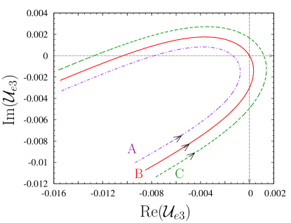
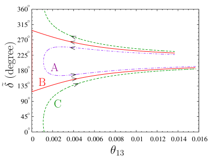
Figure 1: The left panel shows the evolution in the Re$({\cal U}_{e3})$–Im$({\cal U}_{e3})$ parameter plane, whereas The right panel shows the corresponding evolution in the $\theta_{13}$–$\tilde{\delta}$ plane. The values of the parameters chosen at $\mu_{0}=10^{12}$ GeV are: $\tan{\beta}=50$, $m_{0}=0.0585$ eV², ${\Delta m}^{2}_{21}=4.22\times 10^{-5}$ eV², ${\Delta m}^{2}_{32}=3.91\times 10^{-3}$ eV², $\theta_{12}=32.84^{\circ}$, $\theta_{23}=43.71^{\circ}$ and $\theta_{13}=0.014$ rad. The Majorana phases are taken to be $\phi_{1}=58.9^{\circ}$ and $\phi_{2}=159.15^{\circ}$. The Dirac CP phase is $124.0^{\circ}$ for case A (violet, dash-dotted line), $128.447^{\circ}$ for case B (red, solid line) and $133.0^{\circ}$ for case C (green, dashed line).

(a) Though all the parameter values at the high scale are very close, and though in all cases $\theta_{13}$ decreases to a very small value before it starts to increase, $\theta_{13}$ does not vanish during the evolution in all the cases. Indeed, the value of $\delta$ chosen at the high scale, in order to make $\theta_{13}$ vanish during its evolution, needs to be extremely fine-tuned. This is because

$$\sin^{2}\theta_{13}=[{\rm Re}({\cal U}_{e3})]^{2}+[{\rm Im}({\cal U}_{e3})]^{2}\;,$$ (11)

so that one needs both the real and imaginary components of ${\cal U}_{e3}$ to vanish simultaneously, which needs a coincidence. Note that when both the CP violating phases $\delta$ and $\phi_{i}$ vanish at the high scale, Im$({\cal U}_{e3})=0$ automatically throughout the evolution. Then starting from a non-zero value at high scale, $\theta_{13}$ can be made to vanish simply by requiring Re$({\cal U}_{e3})=0$ so that no fine tuning is needed.
(b) With the definition $\tilde{\delta}\equiv 2\pi-\delta$ we have ${\cal U}_{e3}\equiv s_{13}e^{i\tilde{\delta}}$ and thus $\tilde{\delta}$ is the phase of ${\cal U}_{e3}$ which can be read off easily from the Re$({\cal U}_{e3})$–Im$({\cal U}_{e3})$ plot. The values of $\delta$ chosen at $\mu_{0}=10^{12}$ GeV are such that $\tilde{\delta}$ is in the third quadrant, so Re$({\cal U}_{e3})<0$ and Im$({\cal U}_{e3})<0$ at this scale. At the end of the evolution, at $\mu=10^{4}$ GeV, $\tilde{\delta}$ returns to the third quadrant. During its evolution, $\tilde{\delta}$ may change its quadrant zero, one or multiple times. The value of $\theta_{13}$ need not vanish completely during the RG evolution, as is represented by the scenarios A and C. Scenario B is the one where Re$({\cal U}_{e3})$ and Im$({\cal U}_{e3})$ vanish at the same point, and therefore $\theta_{13}$ passes through zero during its evolution.
(c) In scenario A, since Re$({\cal U}_{e3})$ stays negative, $\tilde{\delta}$ simply moves from the third quadrant to the second, and then returns to the third in a continuous manner. In scenario C on the other hand, $\tilde{\delta}$ has to pass through the fourth, first and second quadrant in sequence to finally return to the third quadrant. However its evolution is continuous, the apparent jump at the lowest $\theta_{13}$ values in the right panel of Fig. 1 is just the identification of $0^{\circ}$ and $360^{\circ}$.
(d) In scenario B, $\tilde{\delta}$ starts in the third quadrant and moves continuously to the fourth quadrant. However it propagates to the second quadrant directly through the origin, thus bypassing the first quadrant entirely. Its value at the origin can be well-defined through the limit

$$\cot\tilde{\delta}_{0}\equiv\lim_{{\rm Re}({\cal U}_{e3}),{\rm Im}({\cal U}_{e3})\to 0}\quad\frac{{\rm Re}({\cal U}_{e3})}{{\rm Im}({\cal U}_{e3})}=\lim_{{\rm Re}({\cal U}_{e3}),{\rm Im}({\cal U}_{e3})\to 0}\quad\frac{\frac{d}{dt}{\rm Re}({\cal U}_{e3})}{\frac{d}{dt}{\rm Im}({\cal U}_{e3})}$$ (12)

where we have used L’Hospital’s rule to compute the limit since both the numerator and denominator in this ratio tend to zero at the limiting point.

Since

$${\rm Re}({\cal U}_{e3})=\sin\theta_{13}\cos{\delta}\;,\quad{\rm Im}({\cal U}_{e3})=-\sin\theta_{13}\sin{\delta}\;,$$ (13)

we have

$$\cot\tilde{\delta}_{0}=-\frac{A_{13}\cos\delta-D_{\delta}\sin\delta}{A_{13}\sin\delta+D_{\delta}\cos\delta}\;,$$ (14)

and using eqs. (6) and (10), one obtains

$$\cot\tilde{\delta}_{0}=-\frac{m_{1}\cos{2\phi_{1}}-(1+\zeta)m_{2}\cos{2\phi_{2}}-\zeta m_{3}}{m_{1}\sin{2\phi_{1}}-(1+\zeta)m_{2}\sin{2\phi_{2}}}\;.$$ (15)

Since $\delta=2\pi-\tilde{\delta}$, this is equivalent to

$$\cot\delta_{0}=\frac{m_{1}\cos{2\phi_{1}}-(1+\zeta)m_{2}\cos{2\phi_{2}}-\zeta m_{3}}{m_{1}\sin{2\phi_{1}}-(1+\zeta)m_{2}\sin{2\phi_{2}}}\;,$$ (16)

which corresponds exactly to the value of $\cot\delta$ in eq. (8), which had been prescribed in antusch . We have thus shown that the prescription follows directly from the procedure of taking the limit of $\delta$ as Re$({\cal U}_{e3})$ and Im$({\cal U}_{e3})$ go to zero simultaneously.

The net evolution of $\theta_{13}$ and $\delta$ as functions of the energy scale has been shown in the top panels of Fig. 2. The evolution of $\delta$ clearly has a discontinuity at $\theta_{13}=0$ in scenario B, where its value changes by $\pi$. Though the origin of this discontinuity has now been well understood, it is important to have a clear evolution of parameters that reflect the continuous nature of the evolution of elements of the neutrino mixing matrix $U_{\rm PMNS}$. This can clearly be achieved by using the parameters Re$({\cal U}_{e3})$ and Im$({\cal U}_{e3})$. However, we prefer to use the Jarlskog invariant

$$J_{\rm CP}\equiv\frac{1}{2}\sin{\theta_{12}}\cos{\theta_{12}}\sin{\theta_{23}}\cos{\theta_{23}}\sin{\theta_{13}}\cos^{2}{\theta_{13}}\sin{\delta}\;,$$ (17)

which appears in the probability expressions relevant for the neutrino oscillation experiments, and is therefore more directly measurable than the real and imaginary parts of ${\cal U}_{e3}$. Since $J_{\rm CP}$ has information only about $\sin\delta$, we need its partner

$$J_{\rm CP}^{\prime}\equiv\frac{1}{2}\sin{\theta_{12}}\cos{\theta_{12}}\sin{\theta_{23}}\cos{\theta_{23}}\sin{\theta_{13}}\cos^{2}{\theta_{13}}\cos{\delta}\;,$$ (18)

to keep track of the quadrant in which $\delta$ lies. The evolutions of $(J_{\rm CP},J^{\prime}_{\rm CP})$ are very similar to those of $({\rm Re}({\cal U}_{e3}),{\rm Im}({\cal U}_{e3}))$, as can be seen from the bottom panels of Fig. 2.

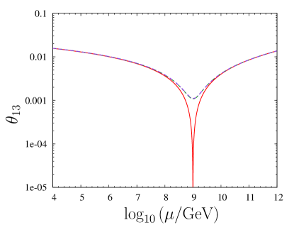
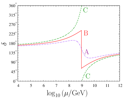
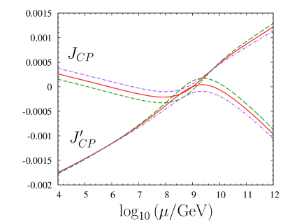
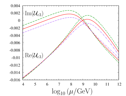
Figure 2: The evolution of $\theta_{13},\delta$, Re$({\cal U}_{e3})$, Im$({\cal U}_{e3})$, $J_{\rm CP}$ and $J^{\prime}_{\rm CP}$ as functions of the energy scale $\mu$, in the scenarios A (violet, dash-dotted line), B (red, solid line) and C (green, dashed line).

III RG evolution equations in terms of the parameter set ${\cal P}_{J}$

We now calculate the RG evolution of the Jarlskog invariant $J_{\rm CP}$ and its partner $J^{\prime}_{\rm CP}$ as defined in (18), and get to a set of evolution equations that are nonsingular everywhere, even at $\theta_{13}=0$. The RG evolution equation for $J_{\rm CP}$ and $J^{\prime}_{\rm CP}$ are obtained as

$$\dot{J}_{\rm CP} = A_{J}+{\cal O}(\theta_{13})\;,$$ (19)

$$\dot{J^{\prime}}_{\rm CP} = A_{J}^{\prime}+{\cal O}(\theta_{13})\;,$$ (20)

with

$$A_{J} = Cy_{\tau}^{2}s_{12}^{2}c_{12}^{2}s_{23}^{2}c_{23}^{2}\frac{m_{3}}{\Delta m^{2}_{31}}\Bigl{[}m_{1}\sin 2\phi_{1}-(1+\zeta)m_{2}\sin 2\phi_{2}\Bigr{]}\;,$$ (21)

$$A_{J}^{\prime} = Cy_{\tau}^{2}s_{12}^{2}c_{12}^{2}s_{23}^{2}c_{23}^{2}\frac{m_{3}}{\Delta m^{2}_{31}}\Bigl{[}m_{1}\cos 2\phi_{1}-(1+\zeta)m_{2}\cos 2\phi_{2}-\zeta m_{3}\Bigr{]}\;.$$ (22)

We also choose to write the RG evolution for $\theta_{13}^{2}$ instead of $\theta_{13}$, as is traditionally done. This quantity turns out to have a nonsingular behaviour at $\theta_{13}=0$. Moreover, since $\theta_{13}\geq 0$ by convention, the complete information about $\theta_{13}$ lies within $\theta_{13}^{2}$. Also, the possible “sign problem” of $\theta_{13}$ is avoided. In terms of the new parameters $J_{\rm CP}$ and $J_{\rm CP}^{\prime}$, the RG evolution equations for $\theta_{13}^{2}$ becomes

$$\dot{{\theta_{13}^{2}}} = A_{13}^{sq}+{\cal O}(\theta_{13}^{2})\;,$$ (23)

$$A^{sq}_{13} = 8Cy_{\tau}^{2}\frac{m_{3}}{\Delta m^{2}_{31}}\Bigl{\{}J_{\rm CP}\left[m_{1}\sin{2\phi_{1}}-(1+\zeta)m_{2}\sin{2\phi_{2}}\right]\Bigr{.}$$ (24)

$$\Bigl{.}+J_{\rm CP}^{\prime}\left[m_{1}\cos{2\phi_{1}}-(1+\zeta)m_{2}\cos{2\phi_{2}}-\zeta m_{3}\right]\Bigr{\}}\;.$$

Thus the evolution equations in basis ${\cal P}_{J}$ are all non-singular and continuous at every point. In particular, even when $\delta$ shows a discontinuity, $J_{\rm CP}$ as well as $J_{\rm CP}^{\prime}$ change in a continuous manner.

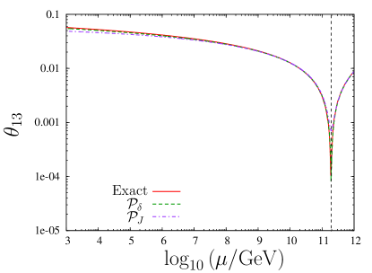
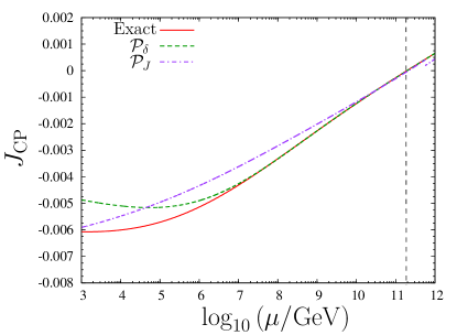
Figure 3: Comparison of the RG evolution of $\theta_{13}$ and $J_{\rm CP}$ from the analytic expressions in ${\cal P}_{\delta}$ basis (green, dashed line) and ${\cal P}_{J}$ basis (blue, dotted line) with the exact numeric one (red, solid line). The parameters chosen at the high scale $\mu_{0}=10^{12}$ GeV are: $\tan{\beta}=50$, $m_{0}=0.05$ eV², ${\Delta m}^{2}_{21}=0.00008$ eV², ${\Delta m}^{2}_{32}=0.0026$ eV², $\theta_{12}=34.5^{\circ}$, $\theta_{23}=42.5^{\circ}$ and $\theta_{13}=0.5^{\circ}$. The phases are taken to be $\delta=40^{\circ}$, $\phi_{1}=25^{\circ}$ and $\phi_{2}=105^{\circ}$.

In Fig. 3, we show the RG evolution of $\theta_{13}$ (left panel) and $J_{\rm CP}$ (right panel), as obtained from the analytic expressions in ${\cal P}_{\delta}$ basis as well as in the ${\cal P}_{J}$ basis, along with the exact numerical solution, for some chosen values of parameters. It shows that the approximate running equations agree with each other to an accuracy of ${\cal O}(\theta_{13})$.

IV Bounds on $\theta_{13}$ at low scale

We now consider all the theories that predict $\theta_{13}=0$ at the high scale and try to see the nature of running of the masses and mixing parameters with the energy scale. For high scale we consider $\mu_{0}=10^{12}$ GeV and implement the symmetry $\theta_{13}=0$ at this scale, which we also take to be the mass of the lightest heavy particle responsible for the seesaw mechanism. We choose this value of $\mu_{0}$ since it is consistent with the current neutrino mass squared differences and seesaw mechanism with Dirac mass of the heaviest neutrino around $1$–$100$ GeV mohapatra-scale . This scale is also desirable for successful leptogenesis buchmuller-scale . However, our results are only logarithmically sensitive to this choice and hence our conclusions will be robust against variations of $\mu_{0}$. Also, this would allow us to compare our bounds with those obtained in qlctbm for specific models like tri-bimaximal mixing at the high scale. The values of the other parameters at high energy are chosen such that their low scale values are compatible with experiments. For the absolute mass scale of neutrinos, we take the cosmological bound of $m_{0}\lesssim 0.5$ eV hannestad at the laboratory energy.

We consider the scenarios where the effective theory below $\mu_{0}$ is the SM or the MSSM. We then estimate the maximum value that $\theta_{13}$ can gain through radiative corrections. This can be obtained from

$$\theta_{13} \equiv \left\arrowvert\int_{t_{0}}^{t}A_{13}dt+{\cal O}(\theta_{13})\right\arrowvert$$ (26)

$$\approx \frac{|C|\Delta_{\tau}}{2}\sin{2\theta_{12}}\sin{2\theta_{23}}\frac{m_{3}}{|\Delta m^{2}_{31}|}\times$$

$$\left\arrowvert m_{1}\cos{(2\phi_{1}-\delta)}-(1+\zeta)m_{2}\cos{(2\phi_{2}-\delta)}-\zeta m_{3}\cos{\delta}\right\arrowvert+{\cal O}(\Delta_{\tau}\theta_{13},\Delta_{\tau}^{2})\;,$$

where $t_{0}\equiv\ln(\mu_{0}/{\rm GeV})/(16\pi^{2})$, $C=-3/2$ for SM and $C=1$ for MSSM. Note that we can use the parameter set ${\cal P}_{\delta}$ here since apart from the starting point, where $\delta$ is unphysical and hence is irrelevant completely, the evolution in terms of this set is also continuous everywhere. Moreover it is convenient to talk about Dirac and Majorana phases while putting bounds on quantities. In eq. (26), $\Delta_{\tau}$ is defined as

$$\Delta_{\tau}^{{\rm SM}}\equiv-\frac{1}{32\pi^{2}}\left(\frac{g_{2}m_{\tau}}{M_{W}}\right)^{2}\ln{\left(\frac{\mu_{0}}{\mu}\right)}$$ (27)

in the SM, where $g_{2}$ is the SU(2)_L gauge coupling, whereas $m_{\tau}$ and $M_{W}$ are the $\tau$ lepton and W boson masses respectively. In the MSSM,

$$\Delta_{\tau}^{{\rm MSSM}}\equiv-\frac{1}{32\pi^{2}}\left(\frac{g_{2}m_{\tau}}{M_{W}}\right)^{2}(1+\tan^{2}{\beta})\ln{\left(\frac{\mu_{0}}{\mu}\right)}\;.$$ (28)

Numerically, one has $\Delta_{\tau}^{\rm SM}\approx-1.4\times 10^{-5}$ and $\Delta_{\tau}^{\rm MSSM}\approx-1.4\times 10^{-5}(1+\tan^{2}\beta)$, where $\tan\beta$ can take values upto $\sim 50$, and so one can treat these quantities as small parameters. We explicitly indicate the neglected powers of these parameters in eq. (26).

In order to get the maximum $\theta_{13}$ value possible, for any value of the lowest neutrino mass $m_{0}$, all the coefficients of the masses $m_{i}$ in eq. (26) should have the same sign (which we choose to be positive) and the maximum possible magnitude. This can be achieved with the choice

$$2\phi_{1}-\delta_{0}=0\;,\quad|2\phi_{2}-\delta_{0}|=\pi\;,$$ (29)

which gives us

$$\theta_{13}^{\rm max} \approx \frac{|C|\Delta_{\tau}}{2}\sin{2\theta_{12}}\sin{2\theta_{23}}\frac{m_{3}}{|\Delta m^{2}_{31}|}\bigl{[}m_{1}+(1+\zeta)m_{2}+|\zeta m_{3}\cos\delta_{0}|\bigr{]}$$ (30)

$$\leq \frac{|C|\Delta_{\tau}}{2}\sin{2\theta_{12}}\sin{2\theta_{23}}\frac{m_{3}}{|\Delta m^{2}_{31}|}\bigl{[}m_{1}+(1+\zeta)m_{2}+|\zeta|m_{3}\bigr{]}\;.$$ (31)

The right hand side of eq. (31) corresponds to choosing the phases shown in Table 2 for eq. (26). As seen, these phases depend only on whether the neutrino mass ordering is normal or inverted, and not on the low energy effective theory (SM or MSSM). However, the value itself will indeed depend on the effective theory considered. Note that in this procedure of bounding $\theta_{13}$, the actual value of $\delta_{0}$ did not need to be used, a considerable simplification achieved at the expense of a small overestimation.

		$\delta$		$\phi_{1}$		$\phi_{2}\phantom{s}$
Normal ordering		$\pi$		$\pi/2$		$0$
Inverted ordering		$0$		$0$		$\pi/2$

Table 2: Phase choices in SM and MSSM that give the maximum radiative correction for $\theta_{13}$.

To estimate $\theta_{13}^{\rm max}$ that can be generated at the low scale, we take the optimal values of the other quantities in their current 3$\sigma$ allowed ranges pdg . We are allowed to do this since the corrections to $\theta_{13}$ due to the evolutions of the other quantities will formally be ${\cal O}(\Delta_{\tau}^{2})$ rgqlc . The quantity that may run quite a bit is $\theta_{12}$, however the running is extremely small in the SM and $\theta_{12}$ always increases in the MSSM, so we use the maximum allowed value of $\sin 2\theta_{12}$ in eq. (31) for our estimation. The values of $m_{1}$, $m_{2}$ and $m_{3}$ depend on ${\Delta m}^{2}_{21}$, ${\Delta m}^{2}_{32}$, $m_{0}$ as well as the chosen mass ordering. The running of masses and the mass squared differences are governed by the Yukawa couplings of up-type quarks and the U(1)_Y and SU(2)_L gauge couplings. For SM, these evolutions depend also on the Higgs boson self coupling, and Yukawa couplings of down-type quarks and charged leptons. But $\theta_{13}$, as given in eq. (31), will be independent of these quantities to the leading order in $\Delta_{\tau}$ and thus considering ${\Delta m}^{2}_{21}$, ${\Delta m}^{2}_{32}$ in the current 3$\sigma$ range is expected to give the correct estimate to this order. This assumption can be seen to be valid a posteriori from the comparison between analytic and numerical results that follow.

IV.1 $\theta_{13}$ at the low scale in the SM

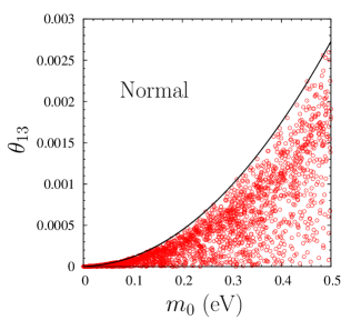
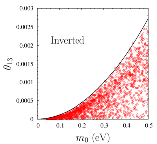
Figure 4: Scatter points show the low energy $\theta_{13}$ as a function of the lightest neutrino mass $m_{0}$ at the low scale, for both normal (left panel) and inverted (right panel) mass ordering. Each point represents a different high energy theory with $\theta_{13}=0$. The solid (black) line gives the maximum attainable $\theta_{13}$ for a given $m_{0}$, calculated using the analytic bound in eq. (31), the current 3$\sigma$ limits of the masses and mixings, and the phase values as given in Table 2.

We first consider the case when the effective low energy theory below $\mu_{0}$ is the SM. Running of the masses and mixing parameters is considered from $\mu_{0}=10^{12}$ GeV to the current experimental scale ($\sim M_{Z}$). The scatter points in Fig. 4 are obtained by keeping $\theta_{13}=0$ and varying the other two mixing angles randomly in the range 0 to $\pi/2$, whereas the phases are varied between 0 to $2\pi$. The masses at the high scale are varied within $0$–$1.0$ eV, so that the lightest neurtino mass $m_{0}$ at the low scale varies between $0$ and $0.5$ eV. Thus each point represents a different high energy theory with $\theta_{13}=0$ at the high scale. The upper bound can be analytically estimated through eq. (31), which depends on the neutrino mass ordering through the phase choices made in Table 2 and the value of $\Delta_{\tau}^{SM}$ is given in eq. (27).

From Fig. 4 it is seen that the maximum value gained radiatively by $\theta_{13}$ is rather small, being $\lesssim 3\times 10^{-3}$ in the range $0\leq m_{0}\leq 0.5$ eV for both the mass orderings. Hence if future experiments measure $\theta_{13}$ greater than this limit, all the theories with $\theta_{13}=0$ at the high scale and SM as the low energy effective theory will be ruled out completely. If the upper limit for $m_{0}$ is brought down by KATRIN katrin to $m_{0}\lesssim 0.2$ eV, even lower $\theta_{13}$ values will be excluded for this class of theories. Note that for $m_{0}$ of this order, the effective electron neutrino mass measured by KATRIN will essentially be the same as $m_{0}$.

IV.2 $\theta_{13}$ at the low scale from MSSM

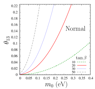
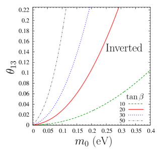
Figure 5: Maximum $\theta_{13}$ obtained at the low scale as a function of the lightest neutrino mass $m_{0}$ at the low scale for $\tan{\beta}$ = $10$, $20$, $30$ and $50$ in the normal (left panel) and inverted (right panel) mass ordering. The plots show that simultaneous measurement of $\theta_{13}$ and $m_{0}$ will help in ruling out of a class of high energy theories with $\theta_{13}=0$. However there is a strong dependence on the upper limit of $\tan{\beta}$.

When MSSM is the low energy effective theory, the evolution of the neutrino parameters is proportional to $(1+\tan^{2}\beta)$, as is seen from eq. (28), where $\tan\beta$ may take values up to $\sim 50$. Thus, considerably larger running of $\theta_{13}$ may be expected at large $\tan\beta$. The variation of $\theta_{13}$ as a function of $m_{0}$ is shown in Fig. 5. From the figure it can be concluded that with the current limit of $m_{0}$, the radiative correction to $\theta_{13}=0$ at the high scale can be large enough to reach the present upper bound of $\theta_{13}$ at laboratory energy. However, for a given $m_{0}\lesssim$ 0.1 eV, the maximum $\theta_{13}$ these theories can generate is significantly lower for the whole $\tan{\beta}$ range. For example, if $m_{0}$ happens to be $0.08$ eV, the maximum $\theta_{13}$ for $\tan\beta=50$ is $\theta_{13}\sim 0.12$, i.e. $\sin^{2}{2\theta_{13}}\sim 0.056$. Such a $\theta_{13}$ regime will be probed by the next generation neutrino oscillation experiments like Double CHOOZ DCHOOZ , Daya Bay daya-bay , T2K t2k . Since the tritium beta decay experiment KATRIN katrin plans to probe $m_{0}\sim 0.2$ eV only, it may not be enough to rule out theories with larger $\tan\beta$.

However, the neutrinoless double beta decay ($0\nu\beta\beta$) experiments will measure the effective Majorana mass of the electron neutrino

$$m_{ee}=\left|c_{12}^{2}c_{13}^{2}m_{1}e^{2i(\phi_{1}-\delta)}+s_{12}^{2}c_{13}^{2}m_{2}e^{2i(\phi_{2}-\delta)}+s_{13}^{2}m_{3}\right|\;,$$ (32)

The value of $m_{ee}$ will allow us to estimate the $m_{0}$ range, albeit with a large uncertainty owing to the complete lack of knowledge of the phases $\delta$, $\phi_{1}$ and $\phi_{2}$ currently. The present upper bound on the average neutrino mass is $m_{ee}<1.1$ eV heidelberg-moscow , whereas the proposed next generation experiments like COBRAcobra , CUORE cuore , EXOexo , GERDA gerda , Super-NEMOs-nemo , MOON moon plan to probe $m_{ee}$ in the range as low as $0.01{\;\rm eV}\leq m_{ee}\leq 0.1{\;\rm eV}$. Therefore, combined measurement of $\theta_{13}$ and $m_{ee}$ may enable us to put some bound on the theories with large $\tan\beta$.

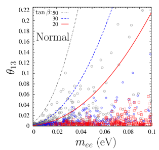
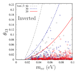
Figure 6: Scatter points show the value of $\theta_{13}$ generated at the low scale as a function of $m_{ee}$, for normal (left panel) and inverted (right panel) ordering. Each point represents a different high energy theory with $\theta_{13}=0$. Different symbols (colors) correspond to different ranges of $\tan{\beta},$ viz. squares (red) for $1.0\leq\tan{\beta}\leq 20.0$, diamonds (blue) for $20.0\leq\tan{\beta}\leq 30.0$ and circles (gray) for $30.0\leq\tan{\beta}\leq 50.0$. The lines show analytic estimates of $\theta_{13}^{\rm max}$: solid (red) line for $\tan{\beta}=20.0$, dashed (blue) line for $\tan{\beta}=30.0$ and dot-dashed (gray) line for $\tan{\beta}=50.0$.

The expression for $m_{ee}$ in (32) can be expanded in terms of the parameter $\delta_{\odot}\equiv{\Delta m}^{2}_{21}/m_{0}^{2}$, which is small in the range $m_{ee}>0.01$ eV, and the small parameter $\theta_{13}$, to get

$$m_{ee}=m_{0}\cos{2\theta_{12}}\left(1-\frac{\delta_{\odot}}{2}\frac{s_{12}^{2}}{\cos{2\theta_{12}}}-\theta_{13}^{2}\right)-\theta_{13}^{2}\sqrt{m_{0}^{2}+{\Delta m}^{2}_{32}}+{\cal O}(\delta_{\odot}^{2},\delta_{\odot}\theta_{13}^{2},\theta_{13}^{3})\;$$ (33)

for normal mass ordering, where the phases are chosen as given in Table 2. For inverted mass ordering,

$$m_{ee}=\cos{2\theta_{12}}(1-\epsilon)\sqrt{m_{0}^{2}+|{\Delta m}^{2}_{32}|}\;+{\cal O}(\delta_{\odot}^{2},\delta_{\odot}\theta_{13}^{2},\theta_{13}^{3})\;,$$ (34)

where

$$\epsilon=\frac{\delta_{\odot}}{2}\frac{c_{12}^{2}}{\cos{2\theta_{12}}(1+\Delta)}+\theta_{13}^{2}\left(1-\frac{1}{\cos{2\theta_{12}}\sqrt{1+\Delta}}\right)\;.$$ (35)

The quantity $\Delta\equiv|{\Delta m}^{2}_{32}|/m_{0}^{2}$ is bounded from below, while for inverted mass ordering $\delta_{\odot}$ is a small parameter ($\sim{\cal O}(10^{-1})$) in the range $m_{ee}>0.02$ eV, so that $\epsilon$ is small in this range. The analytic expressions in eqs. (33) and (34) are valid for $m_{ee}>0.01$ eV and $m_{ee}>0.02$ eV respectively. In this domain of validity, we invert the relations (33) and (34) to obtain $m_{0}$ in terms of $m_{ee}$, and then use eq. (31) for an analytic estimation of $\theta_{13}^{\rm max}$. For the $m_{ee}$ values outside the range of validity, one has to estimate numerically the minimum allowed $m_{ee}$ for a given $m_{0}$ and then use eq. (31) to determine $\theta_{13}^{\rm max}$. These estimations are shown in Fig. 6 for various $\tan\beta$ values. The scattered points are the low scale predictions calculated numerically, which show the correlated constraints in the parameter space of $\theta_{13}$ and $m_{ee}$. It may be noted that the analytic bounds on $\theta_{13}$ obtained here as a function of $m_{ee}$ are generous overestimations, mainly due to the error in the estimation of $m_{0}$ for a given $m_{ee}$.

Note that bounds on $\theta_{13}$ at the low scale generated by RG evolution have been studied earlier in the context of specific neutrino mixing scenarios at the high scale, like the quark-lepton complementarity or tri-bimaximal mixing qlctbm , or correlated generation of $\Delta m^{2}_{21}$ and $\theta_{13}$ Joshipura:2002kj ; Joshipura:2002gr . The bounds obtained in this section, which are applicable not only for all the models with $\theta_{13}=0$ at the high scale, but to all the models with $\theta_{13}=0$ anytime during their RG evolution, subsumes the earlier analyses with specific models.

V Summary

If the neutrino mixing angle $\theta_{13}$ is extremely small, it could point towards some flavor symmetry in the lepton sector. There is indeed a large class of theories of neutrino mass that predict extremely small or even vanishing $\theta_{13}$. However, such predictions are normally valid at the high scale where the masses of the heavy particle responsible for neutrino mass generation lie. Below this scale, radiative corrections give rise to RG evolution of the neutrino mixing parameters, which in principle can wipe out signatures of such symmetries. In this paper, we explore the RG evolution of all such theories collectively.

The RG evolution with the traditional parameter set ${\cal P}_{\delta}=\{m_{i},\theta_{ij},\phi_{i},\delta\}$ involves an apparent singularity in the evolution of the Dirac phase $\delta$ when $\theta_{13}=0$. This singularity is unphysical, since all the elements of the neutrino mixing matrix $U_{\rm PMNS}$ are continuous at $\theta_{13}=0$, and in fact the value of $\delta$ there should be immaterial. A practical solution to this situation has already been proposed, which involves prescribing a specific value of $\cot\delta$ when one starts the RG evolution of a model with $\theta_{13}=0$. However, the rationale behind this prescription has not been studied before in the context of the nature of this apparent singularity. This issue also becomes relevant for the class of models under consideration here, since if $\theta_{13}$ is very close to zero at the high scale, it may vanish completely during its RG evolution, and getting the required value of $\delta$ exactly at that point seems like fine tuning.

We explore the apparent singularity in $\delta$ by analyzing the evolution of the complex quantity ${\cal U}_{e3}$, which stays continuous throughout the RG evolution. We find that a fine tuning is indeed required, but that is to ensure that $\theta_{13}$ exactly vanishes. In general, if the CP violating Dirac and Majorana phases take nontrivial values, one does not pass through $\theta_{13}=0$ even when one starts with $\theta_{13}$ very close to zero. One needs rather finely tuned values for the starting values of the neutrino mixing parameters, unless one introduces a symmetry like CP conservation, which makes the Dirac and Majorana phases vanish everywhere. Since the latter assumption is used commonly in literature, one tends to miss the fact that getting $\theta_{13}=0$ during RG evolution is possible only in a small region of the parameter space.

However, if the parameters happen to be tuned such that $\theta_{13}$ vanishes exactly, we show that the limiting value of $\delta$ as $\theta_{13}\to 0$ is indeed the one given by the prescription mentioned above. We thus put the prescription on a solid footing by deriving it from first principles. We also propose an alternate parametrization using the parameter set ${\cal P}_{J}=\{m_{i},\theta_{12},\theta_{23},\theta_{13}^{2},\phi_{i},J_{\rm CP},J^{\prime}_{\rm CP}\}$, where all the parameters are well-defined everywhere and any seemingly nonsingular behavior is avoided.

For models with exactly vanishing $\theta_{13}$ at the high scale, we study the generation of nonzero $\theta_{13}$ through radiative corrections. We consider two scenarios, one when the low energy effective theory is the SM, and the other where it is the MSSM. The radiatively generated $\theta_{13}$ values are correlated with the absolute neutrino mass scale $m_{0}$. This scale will be probed by the future experiments on tritium beta decay, and indirectly by the neutrinoless double beta decay experiments. If the value of $m_{0}$ is indeed restricted to the value $\sim 0.2$ eV which KATRIN will probe, the maximum value of $\theta_{13}$ generated can only be $\lesssim 3\times 10^{-3}$ in the SM scenario. With the MSSM, the running can be much higher for large $\tan\beta$, such that the current bound of $\theta_{13}<0.22$ may be reached. In this scenario, we correlate the bound on $\theta_{13}$ with the effective neutrino Majorana mass $m_{ee}$ to be measured in the next generation neutrinoless double beta decay experiments. The whole class of models considered in this paper can then be ruled out from future measurements of $\theta_{13},m_{ee}$ and $\tan\beta$.

References

- (1) B. Pontecorvo, Sov. Phys. JETP 7, 172 (1958) [Zh. Eksp. Teor. Fiz. 34, 247 (1957)]; B. Pontecorvo, Sov. Phys. JETP 26, 984 (1968) [Zh. Eksp. Teor. Fiz. 53, 1717 (1967)]; V. N. Gribov and B. Pontecorvo, Phys. Lett. B 28, 493 (1969).
- (2) Z. Maki, M. Nakagawa and S. Sakata, Prog. Theor. Phys. 28, 870 (1962).
- (3) T. Schwetz, M. Tortola and J. W. F. Valle, arXiv:0808.2016 [hep-ph]; G. L. Fogli, E. Lisi, A. Marrone, A. Palazzo and A. M. Rotunno, Phys. Rev. Lett. 101, 141801 (2008) [arXiv:0806.2649 [hep-ph]]; A. Bandyopadhyay, S. Choubey, S. Goswami, S. T. Petcov and D. P. Roy, arXiv:0804.4857 [hep-ph].
- (4) C. H. Albright and M. C. Chen, Phys. Rev. D 74, 113006 (2006) [arXiv:hep-ph/0608137].
- (5) T. Fukuyama and H. Nishiura, arXiv:hep-ph/9702253; R. N. Mohapatra and S. Nussinov, Phys. Rev. D 60, 013002 (1999) [arXiv:hep-ph/9809415]; C. S. Lam, Phys. Lett. B 507, 214 (2001) [arXiv:hep-ph/0104116]; W. Grimus and L. Lavoura, JHEP 0107, 045 (2001) [arXiv:hep-ph/0105212]; W. Grimus and L. Lavoura, Acta Phys. Polon. B 32, 3719 (2001) [arXiv:hep-ph/0110041].
- (6) E. Ma and G. Rajasekaran, Phys. Rev. D 64, 113012 (2001) [arXiv:hep-ph/0106291]; K. S. Babu, E. Ma and J. W. F. Valle, Phys. Lett. B 552, 207 (2003) [arXiv:hep-ph/0206292]; G. Altarelli and F. Feruglio, Nucl. Phys. B 741, 215 (2006) [arXiv:hep-ph/0512103].
- (7) W. Grimus, A. S. Joshipura, S. Kaneko, L. Lavoura and M. Tanimoto, JHEP 0407, 078 (2004) [arXiv:hep-ph/0407112]; H. Ishimori, T. Kobayashi, H. Ohki, Y. Omura, R. Takahashi and M. Tanimoto, Phys. Lett. B 662, 178 (2008) [arXiv:0802.2310 [hep-ph]].
- (8) P. F. Harrison, D. H. Perkins and W. G. Scott, Phys. Lett. B 458, 79 (1999) [arXiv:hep-ph/9904297]; P. F. Harrison, D. H. Perkins and W. G. Scott, Phys. Lett. B 530, 167 (2002) [arXiv:hep-ph/0202074]; W. Grimus and L. Lavoura, JHEP 0508, 013 (2005) [arXiv:hep-ph/0504153]; P. F. Harrison and W. G. Scott, Phys. Lett. B 557, 76 (2003) [arXiv:hep-ph/0302025]; Y. Koide, Phys. Rev. D 73, 057901 (2006) [arXiv:hep-ph/0509214].
- (9) T. Brown, S. Pakvasa, H. Sugawara and Y. Yamanaka, Phys. Rev. D 30, 255 (1984); E. Ma, Phys. Lett. B 632, 352 (2006) [arXiv:hep-ph/0508231]; Y. Koide, JHEP 0708, 086 (2007) [arXiv:0705.2275 [hep-ph]]; C. S. Lam, Phys. Rev. Lett. 101, 121602 (2008) [arXiv:0804.2622 [hep-ph]].
- (10) F. Vissani, JHEP 9811, 025 (1998) [arXiv:hep-ph/9810435].
- (11) S. T. Petcov, Phys. Lett. B 110, 245 (1982); A. S. Joshipura, Phys. Rev. D 60, 053002 (1999) [arXiv:hep-ph/9808261]; A. S. Joshipura and S. D. Rindani, Phys. Lett. B 464, 239 (1999) [arXiv:hep-ph/9907390]; L. Lavoura, Phys. Rev. D 62, 093011 (2000) [arXiv:hep-ph/0005321]; L. Lavoura and W. Grimus, JHEP 0009, 007 (2000) [arXiv:hep-ph/0008020]; G. Altarelli and R. Franceschini, JHEP 0603, 047 (2006) [arXiv:hep-ph/0512202].
- (12) S. Choubey and W. Rodejohann, Eur. Phys. J. C 40, 259 (2005) [arXiv:hep-ph/0411190].
- (13) C. I. Low, Phys. Rev. D 70, 073013 (2004) [arXiv:hep-ph/0404017].
- (14) A. Watanabe and K. Yoshioka, JHEP 0605, 044 (2006) [arXiv:hep-ph/0601152]; R. N. Mohapatra and W. Rodejohann, Phys. Lett. B 644, 59 (2007) [arXiv:hep-ph/0608111]; A. Blum, R. N. Mohapatra and W. Rodejohann, Phys. Rev. D 76, 053003 (2007) [arXiv:0706.3801 [hep-ph]]; G. C. Branco, D. Emmanuel-Costa, M. N. Rebelo and P. Roy, Phys. Rev. D 77, 053011 (2008) [arXiv:0712.0774 [hep-ph]]; S. Goswami and A. Watanabe, arXiv:0807.3438 [hep-ph].
- (15) C. H. Albright and S. M. Barr, Phys. Rev. D 64, 073010 (2001) [arXiv:hep-ph/0104294]; Q. Shafi and Z. Tavartkiladze, Phys. Lett. B 633, 595 (2006) [arXiv:hep-ph/0509237]; N. Oshimo, Nucl. Phys. B 668, 258 (2003) [arXiv:hep-ph/0305166].
- (16) I. Masina, Phys. Lett. B 633, 134 (2006) [arXiv:hep-ph/0508031].
- (17) P. H. Chankowski and Z. Pluciennik, Phys. Lett. B 316, 312 (1993) [arXiv:hep-ph/9306333]; P. H. Chankowski and S. Pokorski, Int. J. Mod. Phys. A 17, 575 (2002) [arXiv:hep-ph/0110249].
- (18) K. S. Babu, C. N. Leung and J. T. Pantaleone, Phys. Lett. B 319, 191 (1993) [arXiv:hep-ph/9309223].
- (19) S. Antusch, M. Drees, J. Kersten, M. Lindner and M. Ratz, Phys. Lett. B 519, 238 (2001) [arXiv:hep-ph/0108005]; S. Antusch, J. Kersten, M. Lindner and M. Ratz, Nucl. Phys. B 674, 401 (2003) [arXiv:hep-ph/0305273].
- (20) S. Antusch, M. Drees, J. Kersten, M. Lindner and M. Ratz, Phys. Lett. B 525, 130 (2002) [arXiv:hep-ph/0110366].
- (21) J. R. Ellis and S. Lola, Phys. Lett. B 458, 310 (1999) [arXiv:hep-ph/9904279]; S. Lola, Acta Phys. Polon. B 31, 1253 (2000) [arXiv:hep-ph/0005093].
- (22) N. Haba and N. Okamura, Eur. Phys. J. C 14, 347 (2000) [arXiv:hep-ph/9906481].
- (23) E. Ma, J. Phys. G 25, L97 (1999) [arXiv:hep-ph/9907400].
- (24) N. Haba, Y. Matsui, N. Okamura and T. Suzuki, Phys. Lett. B 489, 184 (2000) [arXiv:hep-ph/0005064].
- (25) P. H. Chankowski, W. Krolikowski and S. Pokorski, Phys. Lett. B 473, 109 (2000) [arXiv:hep-ph/9910231].
- (26) J. T. Pantaleone, T. K. Kuo and G. H. Wu, Phys. Lett. B 520, 279 (2001) [arXiv:hep-ph/0108137].
- (27) S. Luo and Z. Z. Xing, Phys. Lett. B 637, 279 (2006) [arXiv:hep-ph/0603091].
- (28) F. Vissani, arXiv:hep-ph/9708483.
- (29) G. C. Branco, M. N. Rebelo and J. I. Silva-Marcos, Phys. Rev. Lett. 82, 683 (1999) [arXiv:hep-ph/9810328].
- (30) N. Haba, Y. Matsui, N. Okamura and M. Sugiura, Prog. Theor. Phys. 103, 145 (2000) [arXiv:hep-ph/9908429].
- (31) J. A. Casas, J. R. Espinosa, A. Ibarra and I. Navarro, Nucl. Phys. B 569, 82 (2000) [arXiv:hep-ph/9905381].
- (32) R. Adhikari, E. Ma and G. Rajasekaran, Phys. Lett. B 486, 134 (2000) [arXiv:hep-ph/0004197].
- (33) A. S. Joshipura, S. D. Rindani and N. N. Singh, Nucl. Phys. B 660, 362 (2003) [arXiv:hep-ph/0211378].
- (34) A. S. Joshipura and S. Mohanty, Phys. Rev. D 67, 091302 (2003) [arXiv:hep-ph/0302181].
- (35) Z. Z. Xing and H. Zhang, Commun. Theor. Phys. 48, 525 (2007) [arXiv:hep-ph/0601106].
- (36) S. T. Petcov, T. Shindou and Y. Takanishi, Nucl. Phys. B 738, 219 (2006) [arXiv:hep-ph/0508243].
- (37) M. Tanimoto, Phys. Lett. B 360, 41 (1995) [arXiv:hep-ph/9508247].
- (38) N. Haba, N. Okamura and M. Sugiura, Prog. Theor. Phys. 103, 367 (2000) [arXiv:hep-ph/9810471].
- (39) K. R. S. Balaji, A. S. Dighe, R. N. Mohapatra and M. K. Parida, Phys. Rev. Lett. 84, 5034 (2000) [arXiv:hep-ph/0001310]; K. R. S. Balaji, A. S. Dighe, R. N. Mohapatra and M. K. Parida, Phys. Lett. B 481, 33 (2000) [arXiv:hep-ph/0002177].
- (40) K. R. S. Balaji, R. N. Mohapatra, M. K. Parida and E. A. Paschos, Phys. Rev. D 63, 113002 (2001) [arXiv:hep-ph/0011263].
- (41) R. N. Mohapatra, M. K. Parida and G. Rajasekaran, Phys. Rev. D 69, 053007 (2004) [arXiv:hep-ph/0301234].
- (42) S. K. Agarwalla, M. K. Parida, R. N. Mohapatra and G. Rajasekaran, Phys. Rev. D 75, 033007 (2007) [arXiv:hep-ph/0611225].
- (43) A. S. Joshipura, Phys. Lett. B 543, 276 (2002) [arXiv:hep-ph/0205038].
- (44) A. S. Joshipura and S. D. Rindani, Phys. Rev. D 67, 073009 (2003) [arXiv:hep-ph/0211404].
- (45) J. W. Mei and Z. Z. Xing, Phys. Rev. D 70, 053002 (2004) [arXiv:hep-ph/0404081].
- (46) P. H. Chankowski and P. Wasowicz, Eur. Phys. J. C 23, 249 (2002) [arXiv:hep-ph/0110237].
- (47) S. Antusch, J. Kersten, M. Lindner, M. Ratz and M. A. Schmidt, JHEP 0503, 024 (2005) [arXiv:hep-ph/0501272]; S. Antusch, J. Kersten, M. Lindner and M. Ratz, Phys. Lett. B 538, 87 (2002) [arXiv:hep-ph/0203233].
- (48) R. N. Mohapatra, M. K. Parida and G. Rajasekaran, Phys. Rev. D 71, 057301 (2005) [arXiv:hep-ph/0501275].
- (49) S. Antusch, J. Kersten, M. Lindner and M. Ratz, Phys. Lett. B 544, 1 (2002) [arXiv:hep-ph/0206078].
- (50) T. Miura, T. Shindou and E. Takasugi, Phys. Rev. D 68, 093009 (2003) [arXiv:hep-ph/0308109]; T. Shindou and E. Takasugi, Phys. Rev. D 70, 013005 (2004) [arXiv:hep-ph/0402106].
- (51) V. D. Barger, S. Pakvasa, T. J. Weiler and K. Whisnant, Phys. Lett. B 437, 107 (1998) [arXiv:hep-ph/9806387]; M. Jezabek and Y. Sumino, Phys. Lett. B 457, 139 (1999) [arXiv:hep-ph/9904382].
- (52) A. Dighe, S. Goswami and P. Roy, Phys. Rev. D 73, 071301 (2006) [arXiv:hep-ph/0602062].
- (53) A. Dighe, S. Goswami and W. Rodejohann, Phys. Rev. D 75, 073023 (2007) [arXiv:hep-ph/0612328].
- (54) A. Dighe, S. Goswami and P. Roy, Phys. Rev. D 76, 096005 (2007) [arXiv:0704.3735 [hep-ph]].
- (55) R. N. Mohapatra, N. Setzer and S. Spinner, Phys. Rev. D 73, 075001 (2006) [arXiv:hep-ph/0511260].
- (56) W. Buchmuller, P. Di Bari and M. Plumacher, Nucl. Phys. B 665, 445 (2003) [arXiv:hep-ph/0302092].
- (57) S. Hannestad, Phys. Rev. Lett. 95, 221301 (2005) [arXiv:astro-ph/0505551].
- (58) C. Amsler et al. [Particle Data Group], Phys. Lett. B 667, 1 (2008).
- (59) R. G. H. Robertson [KATRIN Collaboration], J. Phys. Conf. Ser. 120, 052028 (2008) [arXiv:0712.3893 [nucl-ex]].
- (60) J. Maricic [Double Chooz Collaboration], AIP Conf. Proc. 928 (2007) 161.
- (61) D. E. Jaffe [Daya Bay Collaboration], AIP Conf. Proc. 870, 555 (2006).
- (62) M. Zito [T2K Collaboration], J. Phys. Conf. Ser. 110, 082023 (2008).
- (63) H. V. Klapdor-Kleingrothaus [Heidelberg-Moscow Collaboration], Prog. Part. Nucl. Phys. 32, 261 (1994).
- (64) D. Y. Stewart [COBRA Collaboration], Nucl. Instrum. Meth. A 580, 342 (2007).
- (65) O. Cremonesi et al. [CUORICINO Collaboration], Phys. Atom. Nucl. 69, 2083 (2006).
- (66) C. Hall [EXO Collaboration], AIP Conf. Proc. 870, 532 (2006).
- (67) K. Kroninger [GERDA Collaboration], J. Phys. Conf. Ser. 110, 082010 (2008).
- (68) A. S. Barabash [NEMO Collaboration], J. Phys. Conf. Ser. 39, 347 (2006) [arXiv:hep-ex/0602011].
- (69) H. Nakamura et al. [Moon Collaboration], J. Phys. Conf. Ser. 39, 350 (2006).