Abstract

The strong–property–fluctuation theory (SPFT) provides a general framework for estimating the constitutive parameters of a homogenized composite material (HCM). We developed the elastodynamic SPFT for orthotropic HCMs, in order to undertake numerical studies. A specific choice of two–point covariance function — which characterizes the distributional statistics of the generally ellipsoidal particles that constitute the component materials — was implemented. Representative numerical examples revealed that the lowest–order SPFT estimate of the HCM stiffness tensor is qualitatively similar to the estimate provided by the Mori–Tanaka mean–field formalism, but the differences between the two estimates vary as the orthotropic nature of the HCM is accentuated. The second–order SPFT provides a correction to the lowest–order estimate of the HCM stiffness tensor and density. The correction, indicating effective dissipation due to scattering loss, increases as the HCM becomes less orthotropic but decreases as the correlation length becomes smaller.

Keywords: Homogenization; strong–property–fluctuation theory; metamaterials; Mori–Tanaka mean–field formalism.

1 Introduction

How do we estimate the effective constitutive properties of composite materials? This question has long been considered in the context of acoustics, elastodynamics and electromagnetics [1, 2]. An upsurge in interest in this topic has been prompted by the recent proliferation of metamaterials, both as theoretical concepts and as physical entities. An operational definition of a metamaterial is as an artificial composite material which exhibits properties that are not exhibited by its component materials or at least not exhibited to the same extent by its component materials [3]. Metamaterials are often exemplified by homogenized composite materials (HCMs). Typically, metamaterials are associated with constitutive parameter regimes which have not been accessible conventionally. For example, in relation to elastodynamics, metamaterials with negative mass density [4] and negative stiffness [5, 6] have recently been described, whereas negatively–refracting metamaterials have been the subject of intense research activity lately in electromagnetics [7].

We focus here on the effective elastodynamic properties of a composite material. The HCM considered arises in the long–wavelength regime from component materials which are generally orthotropic, viscoelastic and randomly distributed as oriented ellipsoidal particles. Our study is based on the strong–property–fluctuation theory (SPFT) which — by allowing for higher–order characterizations of the distributional statistics of the component materials — provides a multi–scattering approach to homogenization [8]. This distinguishes the SPFT from certain well–known self–consistent approaches to homogenization [9, 10, 11, 12], although we note that more sophisticated self–consistent theories have been proposed in recent years [13, 14, 15]. While the general character of the SPFT approach to homogenization is reminiscent of multi–scattering theories [16, 17, 18], the SPFT provides an estimate of the HCM’s constitutive parameters whereas multi–scattering approaches generally provide effective wavenumbers [19, 20, 21]. A distinctive feature of the SPFT is that it incorporates a renormalized formulation which can accommodate relatively strong variations in the constitutive parameters of the component materials. This is because the perturbative scheme for averaging the renormalized equations in the SPFT is based on parameters which remain small even when there are strong fluctuations in the constitutive parameters describing the component materials. In contrast, conventional variational methods of homogenization [22, 23, 24, 25, 26] yield bounds which are widely separated when there are large differences between the constitutive parameters of the component materials.

The SPFT has been widely utilized to estimate the electromagnetic constitutive parameters of HCMs [27, 28, 29, 30, 31]. Acoustic [32] and elastodynamic [33] versions of the theory have also been developed. The general framework for the elastodynamic SPFT, applicable to linear anisotropic HCMs, was established in 1999 [33], but no numerical studies have been reported hitherto. In the following we apply this theory to examine numerically the case wherein the component materials are generally orthotropic materials which are distributed as oriented ellipsoidal particles. Prior to undertaking our numerical study, we derive new theoretical results in two areas:

• in the implementation of a two–point covariance function which characterizes the distributions of the component materials, and

• in the simplification of certain integrals in order to make them amenable to numerical computation.

The SPFT estimates of the HCM constitutive parameters are illustrated by means of numerical examples, and results are compared to those provided by the Mori–Tanaka mean–field approach [34, 35].

2 Theory

2.1 Preliminaries

In applying the elastodynamic SPFT formalism, it is expedient to adopt both matrix and tensor representations [36]. The correspondence between the two representations is described in Appendix A. Matrixes are denoted by double underlining and bold font, while vectors are in bold font with no underlining. Tensors are represented in normal font with their components indicated by subscripts (for $n$th–order tensors, with $n\leq 4$) or subscripts and superscripts (for eighth–order tensors). All tensor indexes range from $1$ to $3$. The $pq$th component of a matrix $\underline{\underline{\bf A}}$ is written as $\left[\,\underline{\underline{\bf A}}\,\right]_{pq}$, while the $p$th component of a vector ${\bf b}$ is written as $\left[\,{\bf b}\,\right]_{p}$. A repeated index implies summation. Thus, we have the matrix component $\big{[}\,\underline{\underline{\bf A}}\cdot\underline{\underline{\bf B}}\,\big{]}_{pr}=\big{[}\,\underline{\underline{\bf A}}\,\big{]}_{pq}\big{[}\,\underline{\underline{\bf B}}\,\big{]}_{qr}$, vector component $\big{[}\,\underline{\underline{\bf A}}\cdot{\bf b}\big{]}_{p}=\big{[}\,\underline{\underline{\bf A}}\,\big{]}_{pq}\big{[}{\bf b}\big{]}_{q}$, and scalar ${\bf a}\cdot{\bf b}=\left[{\bf a}\right]_{p}\left[{\bf b}\right]_{p}$. The adjoint, determinant and trace of a matrix $\underline{\underline{\bf A}}$ are denoted by $\mbox{adj}\left(\,\underline{\underline{\bf A}}\,\right)$, $\mbox{det}\left(\,\underline{\underline{\bf A}}\,\right)$ and $\mbox{tr}\left(\,\underline{\underline{\bf A}}\,\right)$, respectively. The prefixes Re and Im are used to signify real and imaginary parts, respectively, while $i=\sqrt{-1}$.

The SPFT is developed in the frequency domain wherein the stress, strain, and displacement have an implicit $\exp\left(-i\omega t\right)$ dependency on time $t$, $\omega$ being the angular frequency. Thus, these are generally complex–valued quantities. In order to retrieve the corresponding time–domain quantities, the inverse temporal Fourier transform operation must be performed, although one must bear in mind that homogenization is essentially a long–wavelength procedure [37, 38]. The possibility of viscoelastic behaviour is accommodated through complex–valued constitutive parameters. Stiffness tensors are taken to exhibit the usual symmetries

$$C_{lmpq}=C_{mlpq}=C_{lmqp}=C_{pqlm},$$ (1)

whilst noting that the symmetry $\mbox{Im}\,C_{lmpq}=\mbox{Im}\,C_{pqlm}$ has not been proved generally [39]. On account of the symmetries (1), the matrix counterpart of tensor $C_{lmpq}$ — namely, the 9$\times$9 stiffness matrix $\underline{\underline{\bf C}}$ — is symmetric.

2.2 Component materials

We consider the homogenization of a two–component composite material. The component materials, which are themselves homogeneous, are randomly distributed throughout the mixture as identically–oriented, conformal, ellipsoidal particles. For convenience, the principal axes of the ellipsoidal particles are taken to be aligned with the Cartesian axes. Thus, the surface of each ellipsoidal particle may be parameterized by the vector

$${\bf r}^{(e)}=\eta\underline{\underline{\bf U}}\cdot\hat{{\bf r}},$$ (2)

where $\eta$ is a linear measure of size, $\hat{{\bf r}}$ is the radial unit vector and the diagonal shape matrix

$$\underline{\underline{\bf U}}=\frac{1}{\sqrt[3]{abc}}\left(\begin{array}[]{ccc}a&0&0\\ 0&b&0\\ 0&0&c\\ \end{array}\right),\qquad\qquad(a,b,c\in\mathbb{R}^{+}).$$ (3)

Let the space occupied by the composite material be denoted by $V$. It is partitioned into parts $V^{(1)}$ and $V^{(2)}$ containing the two component materials labelled as ‘1’ and ‘2’, respectively. The distributional statistics of the component materials are described in terms of moments of the characteristic functions

$$\Phi^{(\ell)}({\bf r})=\left\{\begin{array}[]{ll}1,&\qquad{\bf r}\in V^{(\ell)},\\ &\qquad\qquad\qquad\qquad\qquad\qquad(\ell=1,2).\\ 0,&\qquad{\bf r}\not\in V^{(\ell)},\end{array}\right.$$ (4)

The volume fraction of component material $\ell$, namely $f^{(\ell)}$ , is given by the first statistical moment of $\Phi^{(\ell)}$ ; i.e.,

$$\langle\,\Phi^{(\ell)}({\bf r})\,\rangle=f^{(\ell)},\qquad\qquad\left(\ell=1,2\right),$$ (5)

where the angular brackets denote the ensemble average of the quantity enclosed. Notice that $f^{(1)}+f^{(2)}=1$. The second statistical moment of $\Phi^{(\ell)}$ constitutes a two–point covariance function. The physically–motivated form [41]

$$\langle\,\Phi^{(\ell)}({\bf r})\,\Phi^{(\ell)}({\bf r}^{\prime})\,\rangle=\left\{\begin{array}[]{lll}\langle\,\Phi^{(\ell)}({\bf r})\,\rangle\langle\Phi^{(\ell)}({\bf r}^{\prime})\,\rangle\,,&&\hskip 28.45274pt|\,\underline{\underline{U}}^{-1}\cdot\left({\bf r}-{\bf r}^{\prime}\right)|>L\,,\\ &&\\ \langle\,\Phi^{(\ell)}({\bf r})\,\rangle\,,&&\hskip 28.45274pt|\,\underline{\underline{U}}^{-1}\cdot\left({\bf r}-{\bf r}^{\prime}\right)|\leq L\,,\end{array}\right.$$ (6)

is adopted, where $L>0$ is the correlation length which is taken to be much smaller than the elastodynamic wavelengths but larger than the sizes of the component particles. In the context of the electromagnetic SPFT, the specific form of the covariance function has only a secondary influence on estimates of HCM constitutive parameters, for a range of physically–plausible covariance functions [42].

The elastodynamic properties of the component materials ‘1’ and ‘2’ are characterized by their stiffness tensors $C_{lmpq}^{(1)}$ and $C_{lmpq}^{(2)}$ (or, equivalently, their 9$\times$9 stiffness matrixes $\underline{\underline{\bf C}}^{(\ell)}$, $\ell\in\left\{1,2\right\}$), and their densities $\rho^{(1)}$ and $\rho^{(2)}$. The stiffness tensors exhibit the symmetries represented in (1). The component materials are generally orthotropic [40] in the following developments; i.e., the stiffness matrix for each component material may be expressed as

$$\underline{\underline{\bf C}}^{(\ell)}=\left(\begin{array}[]{lll}\underline{\underline{\bf\mathcal{M}}}^{(\ell)}&\underline{\underline{\bf 0}}&\underline{\underline{\bf 0}}\\ \underline{\underline{\bf 0}}&\underline{\underline{\bf\mathcal{D}}}^{(\ell)}&\underline{\underline{\bf\mathcal{D}}}^{(\ell)}\\ \underline{\underline{\bf 0}}&\underline{\underline{\bf\mathcal{D}}}^{(\ell)}&\underline{\underline{\bf\mathcal{D}}}^{(\ell)}\end{array}\right),\qquad\qquad(\ell=1,2),$$ (7)

where $\underline{\underline{\bf\mathcal{M}}}^{(\ell)}$ and $\underline{\underline{\bf\mathcal{D}}}^{(\ell)}$ are symmetric and diagonal 3$\times$3 matrixes, respectively, and $\underline{\underline{\bf 0}}$ is the 3$\times$3 null matrix. For the degenerate case in which the component material ‘$\ell$’ is isotropic, we have

$$\left.\begin{array}[]{l}\left[\underline{\underline{\bf C}}^{(\ell)}\right]_{11}=\left[\underline{\underline{\bf C}}^{(\ell)}\right]_{22}=\left[\underline{\underline{\bf C}}^{(\ell)}\right]_{33}=\lambda^{(\ell)}+2\mu^{(\ell)}\vspace{4pt}\\ \left[\underline{\underline{\bf C}}^{(\ell)}\right]_{12}=\left[\underline{\underline{\bf C}}^{(\ell)}\right]_{13}=\left[\underline{\underline{\bf C}}^{(\ell)}\right]_{23}=\lambda^{(\ell)}\vspace{4pt}\\ \left[\underline{\underline{\bf C}}^{(\ell)}\right]_{44}=\left[\underline{\underline{\bf C}}^{(\ell)}\right]_{55}=\left[\underline{\underline{\bf C}}^{(\ell)}\right]_{66}=\mu^{(\ell)}\end{array}\right\},\qquad\qquad(\ell=1,2),$$ (8)

where $\lambda^{(\ell)}$ and $\mu^{(\ell)}$ are the Lamé constants [43].

2.3 Comparison material

A central concept in the SPFT is that of a homogeneous comparison material. This provides the initial ansatz for an iterative procedure that delivers a succession of SPFT estimates of the constitutive properties of the HCM. As such, the comparison material represents the lowest–order SPFT estimate of the HCM. Since we have taken the component materials to be generally orthotropic and distributed as ellipsoidal particles, the comparison material is generally orthotropic. While this is a physically–reasonable assumption here, we remark that the form of the HCM stiffness tensor may be derived via certain asymptotic approaches to homogenization [44]. The orthotropic comparison material (OCM) is characterized by its stiffness tensor $C^{(ocm)}_{lmpq}$ and density $\rho^{(ocm)}$, with $C^{(ocm)}_{lmpq}$ exhibiting the symmetries (1).

The SPFT formulation exploits the spectral Green function of the OCM, which may be expressed in 3$\times$3 matrix form as

$$\underline{\underline{\bf G}}^{(ocm)}({\bf k})=\Big{[}k^{2}\underline{\underline{\bf a}}({\bf\hat{k}})-\omega^{2}\rho^{(ocm)}{\underline{\underline{\bf I}}}\Big{]}^{-1},$$ (9)

with $\underline{\underline{\bf I}}$ being the 3$\times$3 identity matrix and $\underline{\underline{\bf a}}({\bf\hat{k}})$ the $3\times 3$ matrix with entries

$$\big{[}\,\underline{\underline{\bf a}}({\bf\hat{k}})\,\big{]}_{mp}=\frac{k_{l}C_{lmpq}^{(ocm)}k_{q}}{k^{2}}.$$ (10)

Herein, ${\bf k}=k{\bf\hat{k}}$ $\equiv\left(k_{1},k_{2},k_{3}\right)$ with ${\bf\hat{k}}=(\sin\theta\cos\phi$, $\sin\theta\sin\phi$, $\cos\theta)$. For use later on in §2.4, we remark that $\underline{\underline{\bf G}}^{(ocm)}({\bf k})$ may be conveniently expressed as

$$\underline{\underline{\bf G}}^{(ocm)}({\bf k})=\frac{1}{\Delta({\bf k})}\,\underline{\underline{\bf N}}({\bf k}),$$ (11)

with the 3$\times$3 matrix function

$$\underline{\underline{\bf N}}({\bf k})=k^{4}\mbox{adj}\left[\,\underline{\underline{\bf a}}({\bf\hat{k}})\,\right]+\omega^{2}\rho^{(ocm)}k^{2}\left\{\,\underline{\underline{\bf a}}({\bf\hat{k}})-\mbox{tr}\left[\,\underline{\underline{\bf a}}({\bf\hat{k}})\right]\,\underline{\underline{\bf I}}\,\right\}+\left(\omega^{2}\rho^{(ocm)}\right)^{2}\underline{\underline{\bf I}}$$ (12)

and the scalar function

$$\Delta({\bf k})=k^{6}\mbox{det}\left[\,\underline{\underline{\bf a}}({\bf\hat{k}})\,\right]-\omega^{2}\rho^{(ocm)}\ k^{4}\mbox{tr}\left\{\mbox{adj}\left[\,\underline{\underline{\bf a}}({\bf\hat{k}})\,\right]\right\}+\left(\omega^{2}\rho^{(ocm)}\right)^{2}k^{2}\,\mbox{tr}\left[\,\underline{\underline{\bf a}}({\bf\hat{k}})\right]-\left(\omega^{2}\rho^{(ocm)}\right)^{3}.$$ (13)

A key step in the SPFT — one which facilitates the calculation of $C^{(ocm)}_{lmpq}$ and $\rho^{(ocm)}$ —  is the imposition of the conditions [33, eqs. (2.72),(2.73)]

$$\left\langle\Phi^{(1)}({\bf r})\,\xi_{lmpq}^{(1)}+\Phi^{(2)}({\bf r})\,\xi_{lmpq}^{(2)}\,\right\rangle=0,$$ (14)

$$\left\langle\Phi^{(1)}({\bf r})\left(\rho^{(1)}-\rho^{(ocm)}\right)+\Phi^{(2)}({\bf r})\left(\rho^{(2)}-\rho^{(ocm)}\right)\right\rangle=0,$$ (15)

in order to remove certain secular terms. In (14), the quantities

$$\xi_{lmpq}^{(\ell)}=\left(C_{lmst}^{(\ell)}-C_{lmst}^{(ocm)}\right)\eta_{stpq},\qquad\quad(\ell=1,2),$$ (16)

where $\eta^{(\ell)}_{stpq}$ is given implicitly via

$$e^{(\ell)}_{pq}=\eta^{(\ell)}_{pqst}f^{(\ell)}_{st},$$ (17)

$$f^{(\ell)}_{ij}=e^{(\ell)}_{ij}+S_{ijlm}\left(C_{lmpq}^{(\ell)}-C_{lmpq}^{(ocm)}\right)e^{(\ell)}_{pq},$$ (18)

and the renormalization tensor

$$S_{rstu} = \frac{1}{8\pi}\int_{0}^{2\pi}d\phi\int_{0}^{\pi}d\theta\sin\theta\times$$ (19)

$$\frac{(\underline{\underline{\bf U}}^{-1}\cdot{\bf\hat{k}})_{t}\left\{(\underline{\underline{\bf U}}^{-1}\cdot{\bf\hat{k}})_{s}\big{[}\,\underline{\underline{\bf a}}^{-1}(\underline{\underline{\bf U}}^{-1}\cdot{\bf\hat{k}})\,\big{]}_{ru}+(\underline{\underline{\bf U}}^{-1}\cdot{\bf\hat{k}})_{r}\big{[}\,\underline{\underline{\bf a}}^{-1}(\underline{\underline{\bf U}}^{-1}\cdot{\bf\hat{k}})\,\big{]}_{su}\right\}}{(\underline{\underline{\bf U}}^{-1}\cdot{\bf\hat{k}})\cdot(\underline{\underline{\bf U}}^{-1}\cdot{\bf\hat{k}})}.$$

Upon substituting (16)–(18) into (14), exploiting (5), and after some algebraic manipulations, we obtain

$$f^{(1)}\left[\left(\underline{\underline{\bf C}}^{(1)}-\underline{\underline{\bf C}}^{(ocm)}\right)^{\dagger}+\underline{\underline{\bf S}}\,\right]^{\dagger}=-f^{(2)}\left[\left(\underline{\underline{\bf C}}^{(2)}-\underline{\underline{\bf C}}^{(ocm)}\right)^{\dagger}+\underline{\underline{\bf S}}\,\right]^{\dagger},$$ (20)

wherein the 9$\times$9 matrix equivalents of the tensors $C_{lmpq}^{(ocm)}$ and $S_{rstu}$ (namely, $\underline{\underline{\bf C}}^{(ocm)}$ and $\underline{\underline{\bf S}}$) have been introduced and ^† denotes the matrix operation defined in Appendix A. The OCM stiffness matrix may be extracted from (20) as

$$\underline{\underline{\bf C}}^{(ocm)}=\underline{\underline{\bf C}}^{(1)}+f^{(2)}\left[\,\mbox{\boldmath$\underline{\underline{\bf\tau}}$}+(\underline{\underline{\bf C}}^{(2)}-\underline{\underline{\bf C}}^{(ocm)})\cdot\underline{\underline{\bf S}}\,\right]^{\dagger}\cdot\left(\underline{\underline{\bf C}}^{(1)}-\underline{\underline{\bf C}}^{(2)}\right),$$ (21)

where $\underline{\underline{\bf\tau}}$ is the $9\times 9$ matrix representation of the identity tensor $\tau_{rstu}$, as described in Appendix A. This nonlinear relation (21) can be readily solved for $\underline{\underline{\bf C}}^{(ocm)}$ by numerical procedures, such as the Jacobi method [45].

By combining (5) with (15), it follows immediately that the OCM density is the volume average of the densities of the component materials ‘1’ and ‘2’; i.e.,

$$\rho^{(ocm)}=f^{(1)}\rho^{(1)}+f^{(2)}\rho^{(2)}.$$ (22)

2.4 Second–order SPFT

The expressions for the second–order estimates of the HCM stiffness and density tensors, as derived elsewhere [33, eqs. (2.77),(2.78)], are

$$C^{(spft)}_{lmpq}=C^{(ocm)}_{lmpq}-\frac{\omega^{2}\rho^{(ocm)}}{2}\int d^{3}k\;\frac{k_{t}}{k^{2}}\,B^{lmrs}_{tupq}({\bf k})\,\left[\,\underline{\underline{\bf G}}^{(ocm)}({\bf k})\,\right]_{vu}\left\{k_{s}\left[\,\underline{\underline{\bf a}}^{-1}({\bf\hat{k}})\,\right]_{rv}+k_{r}\left[\,\underline{\underline{\bf a}}^{-1}({\bf\hat{k}})\,\right]_{sv}\right\}$$ (23)

and

$$\rho^{(spft)}_{mp}=\rho^{(ocm)}\delta_{mp}+\omega^{2}\int d^{3}k\;B({\bf k})\left[\underline{\underline{\bf G}}^{(ocm)}({\bf k})\right]_{mp},$$ (24)

respectively, wherein $\delta_{mp}$ is the Kronecker delta function. The eighth–order tensor $B^{lmrs}_{tupq}({\bf k})$ and scalar $B({\bf k})$ represent the spectral covariance functions given as

$$\left.\begin{array}[]{l}\displaystyle{B^{lmrs}_{tupq}({\bf k})=\frac{\left(\xi^{(2)}_{lmrs}-\xi^{(1)}_{lmrs}\right)\left(\xi^{(2)}_{tupq}-\xi^{(1)}_{tupq}\right)}{8\pi^{3}}\int d^{3}R\;\,\Gamma({\bf R})\,\exp\left(-i{\bf k}\cdot{\bf R}\right)\vspace{4pt}}\\ \displaystyle{B({\bf k})=\frac{\left(\rho^{(2)}-\rho^{(1)}\right)^{2}}{8\pi^{3}}\int d^{3}R\;\Gamma({\bf R})\,\exp\left(-i{\bf k}\cdot{\bf R}\right)}\end{array}\right\},$$ (25)

with

$$\Gamma({\bf r}-{\bf r}^{\prime})=\langle\,\Phi^{(1)}({\bf r})\,\Phi^{(1)}({\bf r}^{\prime})\,\rangle-\langle\,\Phi^{(1)}({\bf r})\,\rangle\,\langle\,\Phi^{(1)}({\bf r}^{\prime})\,\rangle\equiv\langle\,\Phi^{(2)}({\bf r})\,\Phi^{(2)}({\bf r}^{\prime})\,\rangle-\langle\,\Phi^{(2)}({\bf r})\,\rangle\,\langle\,\Phi^{(2)}({\bf r}^{\prime})\,\rangle.$$ (26)

We now proceed to simplify the expressions for $C^{(spft)}_{lmpq}$ and $\rho^{(spft)}_{mp}$ presented in (23) and (24), in order to make them numerically tractable. We begin with the integral on the right sides of (25) which, upon implementing the step function–shaped covariance function (6), may be expressed as

$$\int d^{3}R\;\,\Gamma({\bf R})\,\exp\left(-i{\bf k}\cdot{\bf R}\right)=\int_{|{\bf R}|\leq L}d^{3}R\;\exp\left[-i\left(\underline{\underline{\bf U}}\cdot{\bf k}\right)\cdot{\bf R}\right].$$ (27)

Thus, we find that $B^{lmrs}_{tupq}({\bf k})$ and $B({\bf k})$ are given by

$$\left.\begin{array}[]{l}\displaystyle{B^{lmrs}_{tupq}({\bf k})=\frac{f^{(1)}f^{(2)}\left(\xi^{(2)}_{lmrs}-\xi^{(1)}_{lmrs}\right)\left(\xi^{(2)}_{tupq}-\xi^{(1)}_{tupq}\right)}{2\left(\pi k\sigma\right)^{2}}\left[\frac{\sin\left(k\sigma L\right)}{k\sigma}-L\cos\left(k\sigma L\right)\right]\vspace{4pt}}\\ \displaystyle{B({\bf k})=\frac{f^{(1)}f^{(2)}\left(\rho^{(2)}-\rho^{(1)}\right)^{2}}{2\left(\pi k\sigma\right)^{2}}\left[\frac{\sin\left(k\sigma L\right)}{k\sigma}-L\cos\left(k\sigma L\right)\right]}\end{array}\right\},$$ (28)

wherein the scalar function

$$\sigma\equiv\sigma(\theta,\phi)=\sqrt{a^{2}\sin^{2}\theta\cos^{2}\phi+b^{2}\sin^{2}\theta\sin^{2}\phi+c^{2}\cos^{2}\theta}.$$ (29)

Upon substituting (28) into (23) and (24), the integrals therein with respect to $k$ can be evaluated by means of calculus of residues: The roots of $\Delta({\bf k})=0$ give rise to six poles in the complex–$k$ plane, located at $k=\pm p_{1}$, $\pm p_{2}$ and $\pm p_{3}$, chosen such that $\mbox{Re}\;p_{i}\geq 0\;\;(i=1,2,3)$. From (13), we find that.

$$p_{1}^{2} = P_{A}-\frac{1}{3}\left(\frac{2^{1/3}P_{B}}{P_{C}\,\mbox{det}\left[\,\underline{\underline{\bf a}}({\bf\hat{k}})\,\right]}-\frac{P_{C}}{2^{1/3}\,\mbox{det}\left[\,\underline{\underline{\bf a}}({\bf\hat{k}})\,\right]}\right),$$ (30)

$$p_{2}^{2} = P_{A}+\frac{1}{3}\left(\frac{(1+i\sqrt{3})P_{B}}{2^{2/3}P_{C}\,\mbox{det}\left[\,\underline{\underline{\bf a}}({\bf\hat{k}})\,\right]}-\frac{(1-i\sqrt{3})P_{C}}{2^{4/3}\,\mbox{det}\left[\,\underline{\underline{\bf a}}({\bf\hat{k}})\,\right]}\right),$$ (31)

$$p_{3}^{2} = P_{A}+\frac{1}{3}\left(\frac{(1-i\sqrt{3})P_{B}}{2^{2/3}P_{C}\,\mbox{det}\left[\,\underline{\underline{\bf a}}({\bf\hat{k}})\,\right]}-\frac{(1+i\sqrt{3})P_{C}}{2^{4/3}\,\mbox{det}\left[\,\underline{\underline{\bf a}}({\bf\hat{k}})\,\right]}\right),$$ (32)

wherein

$$P_{A} = \frac{\omega^{2}\rho^{(ocm)}\mbox{tr}\left\{\mbox{adj}\left[\,\underline{\underline{\bf a}}({\bf\hat{k}})\,\right]\right\}}{3\,\mbox{det}\left[\,\underline{\underline{\bf a}}({\bf\hat{k}})\,\right]},$$ (33)

$$P_{B} = \left(\omega^{2}\rho^{(ocm)}\right)^{2}\left(3\,\mbox{det}\left[\,\underline{\underline{\bf a}}({\bf\hat{k}})\,\right]\,\mbox{tr}\left[\,\underline{\underline{\bf a}}({\bf\hat{k}})\,\right]-\mbox{tr}\left\{\mbox{adj}\left[\,\underline{\underline{\bf a}}({\bf\hat{k}})\,\right]\right\}^{2}\right),$$ (34)

$$P_{C}^{3} = P_{D}+\sqrt{4P_{B}^{3}+P_{D}^{2}},$$ (35)

$$P_{D} = \left(\omega^{2}\rho^{(ocm)}\right)^{3}\Big{(}2\,\mbox{tr}\left\{\mbox{adj}\left[\,\underline{\underline{\bf a}}({\bf\hat{k}})\,\right]\right\}^{3}$$ (36)

$$-9\,\mbox{det}\left[\,\underline{\underline{\bf a}}({\bf\hat{k}})\,\right]\,\mbox{tr}\left\{\mbox{adj}\left[\,\underline{\underline{\bf a}}({\bf\hat{k}})\,\right]\right\}\,\mbox{tr}\left[\,\underline{\underline{\bf a}}({\bf\hat{k}})\,\right]+27\,\mbox{det}\left[\,\underline{\underline{\bf a}}({\bf\hat{k}})\,\right]^{2}\Big{)}.$$

Thus, by application of the Cauchy residue theorem [46], the SPFT estimates are delivered as

$$C^{(spft)}_{lmpq} = C^{(ocm)}_{lmpq}+\frac{\omega^{2}\rho^{(ocm)}f^{(1)}f^{(2)}\left(\xi^{(2)}_{lmrs}-\xi^{(1)}_{lmrs}\right)\left(\xi^{(2)}_{tupq}-\xi^{(1)}_{tupq}\right)}{4\pi i}\times$$ (37)

$$\int_{\phi=0}^{2\pi}\int_{\theta=0}^{\pi}d\phi\,d\theta\,\frac{k_{t}\sin\theta\left\{k_{s}\left[\,\underline{\underline{\bf a}}^{-1}({\bf\hat{k}})\,\right]_{rv}+k_{r}\left[\,\underline{\underline{\bf a}}^{-1}({\bf\hat{k}})\,\right]_{sv}\right\}}{\left(k\sigma\right)^{2}\;\mbox{det}\left[\,\underline{\underline{\bf a}}({\bf\hat{k}})\,\right]}\left[\,\underline{\underline{\bf b}}({\bf\hat{k}})\,\right]_{vu},$$

and

$$\rho^{(spft)}_{mp} = \rho^{(ocm)}\delta_{mp}-\frac{\omega^{2}f^{(1)}f^{(2)}\left(\rho^{(2)}-\rho^{(1)}\right)^{2}}{2\pi i}\int_{\phi=0}^{2\pi}\int_{\theta=0}^{\pi}d\phi\,d\theta\,\frac{\sin\theta}{\mbox{det}\left[\,\underline{\underline{\bf a}}({\bf\hat{k}})\,\right]}\,\left[\,\underline{\underline{\bf b}}({\bf\hat{k}})\,\right]_{mp},$$ (38)

where

$$\underline{\underline{\bf b}}({\bf\hat{k}}) = \frac{1}{2i}\bigg{[}\frac{e^{iL\sigma p_{1}}\underline{\underline{\bf N}}(p_{1}\underline{\underline{\bf U}}\cdot{\bf\hat{k}})}{\sigma p_{1}^{2}(p_{1}^{2}-p_{2}^{2})(p_{1}^{2}-p_{3}^{2})}\bigg{(}1-iL\sigma p_{1}\bigg{)}-\frac{e^{iL\sigma p_{2}}\underline{\underline{\bf N}}(p_{2}\underline{\underline{\bf U}}\cdot{\bf\hat{k}})}{\sigma p_{2}^{2}(p_{1}^{2}-p_{2}^{2})(p_{2}^{2}-p_{3}^{2})}\bigg{(}1-iL\sigma p_{2}\bigg{)}$$ (39)

$$+\frac{e^{iL\sigma p_{3}}\underline{\underline{\bf N}}(p_{3}\underline{\underline{\bf U}}\cdot{\bf\hat{k}})}{\sigma p_{3}^{2}(p_{2}^{2}-p_{3}^{2})(p_{1}^{2}-p_{3}^{2})}\bigg{(}1-iL\sigma p_{3}\bigg{)}-\frac{\underline{\underline{\bf N}}({\bf 0})}{\sigma p_{1}^{2}p_{2}^{2}p_{3}^{2}}\bigg{]}.$$

The integrals in (37) and (38) are readily evaluated by standard numerical methods [47].

Significantly, the second–order SPFT estimates $C^{(spft)}_{lmpq}$ and $\rho^{(spft)}_{mp}$ are complex–valued even when the corresponding quantities for the component materials, i.e., $C^{(\ell)}_{lmpq}$ and $\rho^{(\ell)}$ ($\ell=1,2$), are real–valued. This reflects the fact that the SPFT effectively takes into account losses due to scattering. This feature is not unique to the SPFT: it arises generally in multi–scattering approaches to homogenization [16, 20, 48]. We note that for [39]

• the time–averaged strain energy density to be positive–valued, $\mbox{Re}\,\underline{\underline{\bf\breve{C}}}^{(spft)}$ is required to be positive–definite; and

• the time–averaged dissipated energy density to be positive–valued, $-\mbox{Im}\,\underline{\underline{\bf\breve{C}}}^{(spft)}$ is required to be positive–semi–definite,

where $\underline{\underline{\bf\breve{C}}}^{(spft)}$ is the 6$\times$6 matrix with components $\left[\,\underline{\underline{\bf\breve{C}}}^{(spft)}\,\right]_{st}=\left[\,\underline{\underline{\bf C}}^{(spft)}\,\right]_{st}$ $(s,t\in\left\{1,2,\ldots,6\right\})$ and $\underline{\underline{\bf C}}^{(spft)}$ is the 9$\times$9 matrix equivalent to the SPFT stiffness tensor $C^{(spft)}_{lmpq}$.

It is notable too that the second–order SPFT estimates $C^{(spft)}_{lmpq}$ and $\rho^{(spft)}_{mp}$ are explicitly dependent on frequency, whereas the corresponding zeroth–order SPFT estimates exhibit only an implicit dependency on frequency via the frequency–dependent constitutive parameters of the component materials. Accordingly, the second–order SPFT estimates may be viewed as low frequency corrections to the quasi–static estimates provided by the the zeroth–order SPFT.

A complex–valued anisotropic density, as delivered by (38), is not without precedent [49]; see Milton [50] for a discussion on this issue.

3 Numerical results

Let us now illustrate the theory presented in §2 by means of some representative numerical examples. We consider homogenizations wherein the component materials are acetal and glass (or orthotropic perturbations of these in §3.2). The corresponding results are qualitatively similar to those we found from homogenizations involving a wide range of different component materials, characterized by widely different constitutive parameters, which are not presented here. In order to provide a baseline for the SPFT estimate of the HCM stiffness tensor, the corresponding results provided by the Mori–Tanaka mean–field formalism [34, 35] were also computed. The Mori–Tanaka formalism was chosen as a comparison for the SPFT because it is well–established and straightforwardly implemented [36, 51]. Comparative studies involving the Mori–Tanaka and other homogenization formalisms are reported elsewhere; see [52, 53, 54], for example. The Mori–Tanaka estimate of the 9$\times$9 stiffness matrix of the HCM may be written as [51]

$$\underline{\underline{\bf C}}^{(MT)}=\left[\,f^{(1)}\underline{\underline{\bf C}}^{(1)}+f^{(2)}\underline{\underline{\bf C}}^{(2)}\cdot\underline{\underline{\bf A}}\,\right]\cdot\left[\,f^{(1)}{\mbox{\boldmath$\underline{\underline{\bf\tau}}$}}+f^{(2)}\underline{\underline{\bf A}}\,\right]^{\dagger},$$ (40)

where

$$\underline{\underline{\bf A}}=\left[\,{\mbox{\boldmath$\underline{\underline{\bf\tau}}$}}+\underline{\underline{\bf S}}^{(esh)}\cdot\left(\underline{\underline{\bf C}}^{(1)}\right)^{\dagger}\cdot\left(\underline{\underline{\bf C}}^{(2)}-\underline{\underline{\bf C}}^{(1)}\right)\,\right]^{\dagger},$$ (41)

and $\underline{\underline{\bf S}}^{(esh)}$ is the 9$\times$9 Eshelby matrix [55]. The evaluation of this matrix is described in Appendix B.

In the remainder of this section, we present the 9$\times$9 stiffness matrix of the HCM, namely $\underline{\underline{\bf C}}^{(hcm)}$, as estimated by the lowest–order SPFT (i.e., $hcm=ocm$), the second–order SPFT (i.e., $hcm=spft$) and the Mori–Tanaka mean–field formalism (i.e., $hcm=MT$). The matrix $\underline{\underline{\bf C}}^{(hcm)}$ generally has the orthotropic form represented in (7) with $\ell=hcm$. We also present the second–order SPFT density tensor $\rho^{(spft)}_{mp}$; numerical results for the lowest–order SPFT density $\rho^{(ocm)}$ need not be presented here as that quantity is simply the volume average of the densities of the component materials. For all second–order SPFT computations, we selected $\omega=2\pi\times 10^{6}$ $\mbox{s}^{-1}$.

3.1 Isotropic component materials distributed as oriented ellipsoidal particles

Let us begin by considering the scenario in which the component materials are both isotropic. The component material ‘1’ is taken to be acetal (i.e., $\lambda^{(1)}=\lambda^{(ace)}$, $\mu^{(1)}=\mu^{(ace)}$ and $\rho^{(1)}=\rho^{(ace)}$), and component material ‘2’ to be glass (i.e., $\lambda^{(2)}=\lambda^{(gla)}$, $\mu^{(2)}=\mu^{(gla)}$ and $\rho^{(2)}=\rho^{(gla)}$). The Lamé constants and densities for these two materials are as follows [56, 57]:

$$\left.\begin{array}[]{lll}\lambda^{(ace)}=2.68\;\mbox{GPa},&\mu^{(ace)}=1.15\;\mbox{GPa},&\rho^{(ace)}=1.43\times 10^{3}\;\mbox{kg}\,\mbox{m}^{-3}\vspace{4pt}\\ \lambda^{(gla)}=21.73\;\mbox{GPa},&\mu^{(gla)}=29.2\;\mbox{GPa},&\rho^{(gla)}=2.23\times 10^{3}\;\mbox{kg}\,\mbox{m}^{-3}\end{array}\right\}.$$ (42)

The eccentricities of the ellipsoidal component particles are specified by the parameters $\left\{a,b,c\right\}$, per (2) and (3).

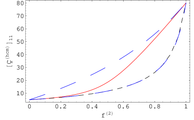
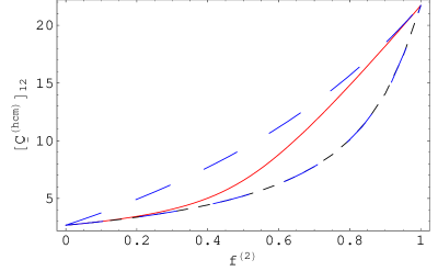
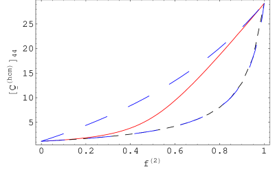
Figure 1: Plots of $\left[\,\underline{\underline{\bf C}}^{(hcm)}\,\right]_{11}$, $\left[\,\underline{\underline{\bf C}}^{(hcm)}\,\right]_{12}$ and $\left[\,\underline{\underline{\bf C}}^{(hcm)}\,\right]_{44}$ (in GPa) as estimated using the lowest–order SPFT (i.e., $hcm=ocm$) (red, solid curves) and the Mori–Tanaka mean–field formalism (i.e., $hcm=MT$) (black, dashed curves), against the volume fraction of component material ‘2’. Also plotted are the upper and lower Hashin–Shtrikman bounds (blue, long dashed curves) for $\left[\,\underline{\underline{\bf C}}^{(hcm)}\,\right]_{11}$ and $\left[\,\underline{\underline{\bf C}}^{(hcm)}\,\right]_{44}$; the lower Hashin–Shtrikman bounds coincide with the Mori–Tanaka estimates. Component material ‘1’ is acetal and component material ‘2’ is glass, as specified in (42). The component materials are distributed as spheres (i.e., $a=b=c$).

In Fig. 1 the components of the HCM stiffness matrix $\underline{\underline{\bf C}}^{(hcm)}$, as computed using the lowest–order SPFT and the Mori–Tanaka formalism, are plotted as functions of volume fraction $f^{(2)}$ for the case $a=b=c$. Since the HCM is isotropic in this case, only the components $\left[\,\underline{\underline{\bf C}}^{(hcm)}\,\right]_{11}\equiv\lambda^{(hcm)}+2\mu^{(hcm)}$, $\left[\,\underline{\underline{\bf C}}^{(hcm)}\,\right]_{12}\equiv\lambda^{(hcm)}$ and $\left[\,\underline{\underline{\bf C}}^{(hcm)}\,\right]_{44}\equiv\mu^{(hcm)}$ are presented, per (8) with $\ell=hcm$. Notice that the following limits necessarily apply for both the SPFT and Mori–Tanaka estimates:

$$\lim_{f^{(2)}\to 0}\underline{\underline{\bf C}}^{(hcm)}=\underline{\underline{\bf C}}^{(1)},\qquad\lim_{f^{(2)}\to 1}\underline{\underline{\bf C}}^{(hcm)}=\underline{\underline{\bf C}}^{(2)}.$$ (43)

It is apparent from Fig. 1 that, while the lowest–order SPFT and the Mori–Tanaka estimates are qualitatively similar, the Mori–Tanaka estimates display a greater deviation from the naive HCM estimate $f^{(1)}\left[\,\underline{\underline{\bf C}}^{(1)}\,\right]_{pq}+f^{(2)}\left[\,\underline{\underline{\bf C}}^{(2)}\,\right]_{pq}$ for mid–range values of $f^{(2)}$. For further comparison in this isotropic scenario, the familiar variational bounds on $\left[\,\underline{\underline{\bf C}}^{(hcm)}\,\right]_{11}$ and $\left[\,\underline{\underline{\bf C}}^{(hcm)}\,\right]_{44}$ established by Hashin and Shtrikman [2, 22] are also presented in Fig. 1: the lower Hashin–Shtrikman bound coincides with the Mori–Tanaka estimate and the lowest–order SPFT estimate lies within the upper and lower Hashin–Shtrikman bounds for all values of $f^{(2)}$. Parenthetically, we note that for isotropic HCMs the lowest–order SPFT estimates are the same as those provided by the well–known formalisms of Hill [9] and Budiansky [11], as demonstrated elsewhere [33].

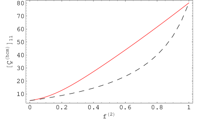
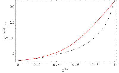
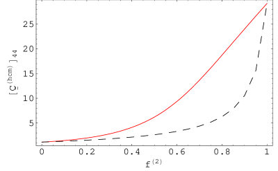
Figure 2: Plots of $\left[\,\underline{\underline{\bf C}}^{(hcm)}\,\right]_{rs}$, with $rs\in\left\{11,12,44\right\}$ (in GPa) as estimated using the lowest–order SPFT (i.e., $hcm=ocm$) (red, solid curves) and the Mori–Tanaka mean–field formalism (i.e., $hcm=MT$) (black, dashed curves), against the volume fraction of component medium ‘2’. Component material ‘1’ is acetal and component material ‘2’ is glass, as specified in (42). The component materials are distributed as ellipsoids with $a/c=5$ and $b/c=1.5$.

The corresponding lowest–order SPFT and Mori–Tanaka estimates for the orthotropic HCM arising from the distribution of component material as ellipsoids described by $\left\{a/c=5,\,b/c=1.5\right\}$ are presented in Fig. 2. The matrix entries $\left[\,\underline{\underline{\bf C}}^{(hcm)}\,\right]_{pq}$ are plotted against $f^{(2)}$ for $pq\in\left\{11,12,44\right\}$. The graphs for $pq=13$ and $23$ are qualitatively similar to those for $pq=12$; and those for $pq=55$ and $66$ are qualitatively similar to those for $pq=44$. The degree of orthotropy exhibited by the HCM can be gauged by relative differences in the values of $\left[\,\underline{\underline{\bf C}}^{(hcm)}\,\right]_{pq}$ for $pq\in\left\{11,\,22,\,33\right\}$ (and similarly by relative differences in $\left[\,\underline{\underline{\bf C}}^{(hcm)}\,\right]_{pq}$ for $pq\in\left\{44,\,55,\,66\right\}$ and by relative differences in $\left[\,\underline{\underline{\bf C}}^{(hcm)}\,\right]_{pq}$ for $pq\in\left\{12,\,13,\,23\right\}$). These relative differences are greatest for mid–range values of the volume fraction $f^{(2)}$.

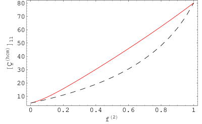
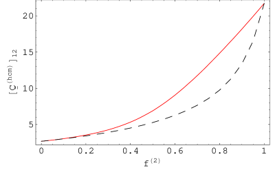
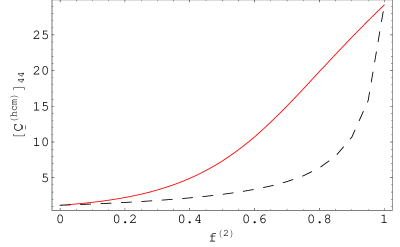
Figure 3: As Fig. 2 but for ellipsoidal component particles specified by $a/c=10$ and $b/c=2$.

The orthotropic nature of the HCM is accentuated by using component materials with more eccentrically–shaped particles. This is illustrated by Fig. 3, which shows results computed for the same scenario as for Fig. 2 but with ellipsoidal particles described by $\left\{a/c=10,\,b/c=2\right\}$. A comparison of Figs. 1–3 reveals that differences between the estimates of the lowest–order SPFT and the Mori–Tanaka mean–field formalism vary slightly as the orthotropic nature of the HCM is accentuated. For example, the difference between the lowest–order SPFT and the Mori–Tanaka estimates of the $\left[\,\underline{\underline{\bf C}}^{(hcm)}\,\right]_{44}$ increases as the HCM becomes more orthotropic.

Now let us turn to the second–order SPFT estimates of the HCM constitutive parameters. We considered these quantities as functions of $\bar{k}L$, where

$$\bar{k}=\frac{\omega}{4}\left(\sqrt{\frac{\rho^{(1)}}{\lambda^{(1)}+2\mu^{(1)}}}+\sqrt{\frac{\rho^{(1)}}{\mu^{(1)}}}+\sqrt{\frac{\rho^{(2)}}{\lambda^{(2)}+2\mu^{(2)}}}+\sqrt{\frac{\rho^{(2)}}{\mu^{(2)}}}\right)$$ (44)

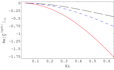
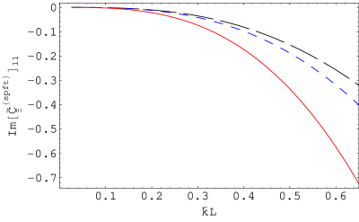
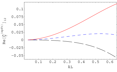
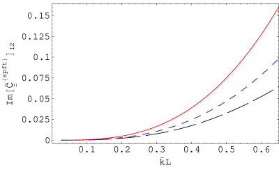
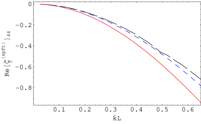
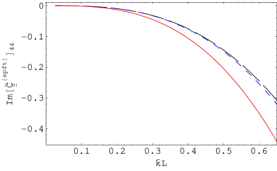
Figure 4: The real and imaginary parts of $\left[\underline{\underline{\bf\tilde{C}}}^{(spft)}\,\right]_{rs}$, with $rs\in\left\{11,12,44\right\}$ (in GPa), plotted as functions of $\bar{k}L$, for $f^{(2)}=0.5$. Component medium ‘1’ is acetal and component medium ‘2’ is glass, as specified in (42). The component materials are distributed as (i) spheres (i.e., $a=b=c$) (red, solid curves), or (ii) ellipsoids with shape parameters $\left\{a/c=5,\,b/c=1.5\right\}$ (blue, short–dashed curves), or (iii) ellipsoids with shape parameters $\left\{a/c=10,\,b/c=2\right\}$ (black, long–dashed curves).

is an approximate wavenumber calculated as the average of the shear and longitudinal wavenumbers in the component materials, and $L$ is the correlation length associated with the the two–point covariance function (6). Since $L$ is required to be smaller than characteristic wavelengths in the HCM (but larger than the sizes of the component particles), we restrict our attention to $0<\bar{k}L<0.6$. Fig. 4 shows the real and imaginary parts of the components of $\underline{\underline{\bf\tilde{C}}}^{(spft)}=\underline{\underline{\bf C}}^{(spft)}-\underline{\underline{\bf C}}^{(ocm)}$ plotted against $\bar{k}L$ for $f^{(2)}=0.5$. The values of the shape parameters $\left\{a,\,b,\,c\right\}$ correspond to those used in the calculations for Figs. 1–3. As previously, only the matrix entries $\left[\,\underline{\underline{\bf\tilde{C}}}^{(spft)}\,\right]_{pq}$ are presented for $pq\in\left\{11,12,44\right\}$. The graphs for $pq=13$ and $23$ are qualitatively similar to those for $pq=12$; and those for $pq=55$ and $66$ are qualitatively similar to those for $pq=44$. Notice that

$$\lim_{L\to 0}\underline{\underline{\bf C}}^{(spft)}=\underline{\underline{\bf C}}^{(ocm)}$$ (45)

and

$$\Big{|}\left[\,\underline{\underline{\bf\tilde{C}}}^{(spft)}\,\right]_{pq}\Big{|}\ll\Big{|}\left[\,\underline{\underline{\bf C}}^{(ocm)}\,\right]_{pq}\Big{|}$$ (46)

for all nonzero matrix entries. Furthermore, for the particular example considered here, the magnitude of $\left[\,\underline{\underline{\bf\tilde{C}}}^{(spft)}\,\right]_{pq}$ generally decreases as the particles of the component materials become more eccentric in shape.

A very striking feature of the second–order SPFT estimates presented in Fig. 4 is that

$$\mbox{Im }\left[\,\underline{\underline{\bf C}}^{(spft)}\,\right]_{pq}\neq 0,$$ (47)

whereas $\mbox{Im }\,\left[\,\underline{\underline{\bf C}}^{(a,b)}\,\right]_{pq}=\mbox{Im }\,\left[\,\underline{\underline{\bf C}}^{(ocm)}\,\right]_{pq}=0$. Furthermore, the magnitude of $\mbox{Im }\left[\,\underline{\underline{\bf C}}^{(spft)}\,\right]_{pq}$ grows steadily as the correlation length increases from zero. These observations may be interpreted in terms of effective losses due to scattering as follows. For all reported calculations, $\mbox{Re}\,\underline{\underline{\bf\breve{C}}}^{(spft)}$ is positive–definite and $-\mbox{Im}\,\underline{\underline{\bf\breve{C}}}^{(spft)}$ is positive–semi–definite, which together imply that the associated time–averaged strain energy and dissipated energy densities are positive–valued [39], as discussed in §2.4. Accordingly, the emergence of nonzero imaginary parts of $\left[\,\underline{\underline{\bf C}}^{(spft)}\,\right]_{pq}$ indicates that the HCM has acquired an effectively dissipative nature, despite the component materials being nondissipative. This effective dissipation must be a scattering loss, because the second–order SPFT accommodates interactions between spatially–distinct scattering centres via the two–point covariance function (6). As the correlation length increases, the number of scattering centres that can mutually interact also increases, thereby increasing the scattering loss per unit volume.

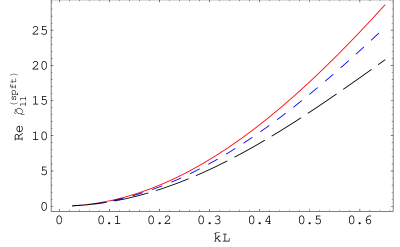
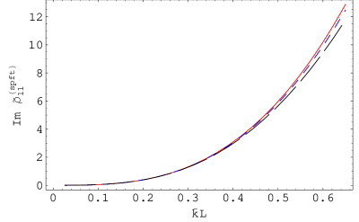
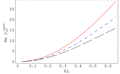
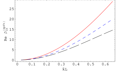
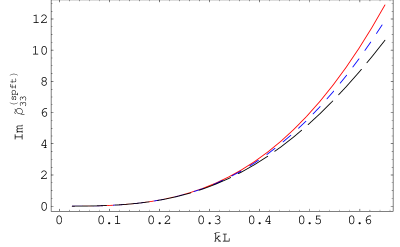
Figure 5: As Fig. 4 but the quantities plotted are the real and imaginary parts of the excess of the second–order SPFT density tensor over the density of the comparison material, i.e., $\tilde{\rho}^{(spft)}_{rr}=\rho^{(spft)}_{rr}-\rho^{(ocm)}$, ($r\in\left\{1,2,3\right\}$), in $\mbox{kg}\,\mbox{m}^{-3}$.

Lastly in this subsection, the real and imaginary parts of the second–order SPFT density tensor $\tilde{\rho}^{(spft)}_{pq}=\rho^{(spft)}_{pq}-\rho^{(ocm)}$ are plotted as functions of $\bar{k}L$ in Fig. 5. Only the $p=q$ components are presented, as the $p\neq q$ components are negligibly small. The density tensor exhibits characteristics similar to those of the corresponding stiffness tensor insofar as

$$\lim_{L\to 0}\rho^{(spft)}_{pq}=\rho^{(ocm)}$$ (48)

and

$$\Big{|}\tilde{\rho}^{(spft)}_{pq}\Big{|}\ll\Big{|}\rho^{(ocm)}\Big{|}$$ (49)

for all values of the indexes $p$ and $q$. Also, $\displaystyle{|\tilde{\rho}^{(spft)}_{pq}|}$ generally decreases as the shape of the particles of the component materials deviates further from spherical.

3.2 Orthotropic component materials distributed as spheres

Let us now explore the scenario wherein the component materials are orthotropic perturbations of the isotropic component materials considered in §3.1. In the notation of (7), we choose

$$\left.\begin{array}[]{l}\underline{\underline{\bf\mathcal{M}}}^{(1)}=\left(\begin{array}[]{lll}\left(\lambda^{(ace)}+2\mu^{(ace)}\right)\left(1+\varsigma\right)&\lambda^{(ace)}\left(1-\varsigma\right)&\lambda^{(ace)}\left(1+2\varsigma\right)\\ \lambda^{(ace)}\left(1-\varsigma\right)&\left(\lambda^{(ace)}+2\mu^{(ace)}\right)\left(1-\frac{1}{4}\varsigma\right)&\lambda^{(ace)}\left(1+\frac{1}{4}\varsigma\right)\\ \lambda^{(ace)}\left(1+2\varsigma\right)&\lambda^{(ace)}\left(1+\frac{1}{4}\varsigma\right)&\left(\lambda^{(ace)}+2\mu^{(ace)}\right)\left(1-2\varsigma\right)\end{array}\right)\vspace{8pt}\\ \underline{\underline{\bf\mathcal{D}}}^{(1)}=\left(\begin{array}[]{lll}\left(\mu^{(ace)}\right)\left(1-\varsigma\right)&0&0\\ 0&\mu^{(ace)}\left(1-\frac{1}{2}\varsigma\right)&0\\ 0&0&\mu^{(ace)}\left(1-\frac{2}{3}\varsigma\right)\end{array}\right)\end{array}\right\}$$ (50)

and

$$\left.\begin{array}[]{l}\underline{\underline{\bf\mathcal{M}}}^{(2)}=\left(\begin{array}[]{lll}\left(\lambda^{(gla)}+2\mu^{(gla)}\right)\left(1+2\varsigma\right)&\lambda^{(gla)}\left(1-2\varsigma\right)&\lambda^{(gla)}\left(1+\frac{1}{2}\varsigma\right)\\ \lambda^{(gla)}\left(1-2\varsigma\right)&\left(\lambda^{(gla)}+2\mu^{(gla)}\right)\left(1+\frac{1}{3}\varsigma\right)&\lambda^{(gla)}\left(1-\frac{1}{3}\varsigma\right)\\ \lambda^{(gla)}\left(1+\frac{1}{2}\varsigma\right)&\lambda^{(gla)}\left(1-\frac{1}{3}\varsigma\right)&\left(\lambda^{(gla)}+2\mu^{(gla)}\right)\left(1-\frac{1}{2}\varsigma\right)\end{array}\right)\vspace{8pt}\\ \underline{\underline{\bf\mathcal{D}}}^{(2)}=\left(\begin{array}[]{lll}\left(\mu^{(gla)}\right)\left(1-\frac{3}{2}\varsigma\right)&0&0\\ 0&\mu^{(gla)}\left(1-\frac{4}{5}\varsigma\right)&0\\ 0&0&\mu^{(gla)}\left(1-\frac{2}{3}\varsigma\right)\end{array}\right)\end{array}\right\},$$ (51)

where the real–valued scalar $\varsigma$ controls the degree of orthotropy. Thus, at fixed values of $\varsigma$ the component materials may be viewed as being locally orthotropic. As in §3.1, the densities of the component materials are taken to be $\rho^{(1)}=\rho^{(ace)}$ and $\rho^{(2)}=\rho^{(gla)}$. The component materials are distributed as spherical particles (i.e., $a=b=c$).

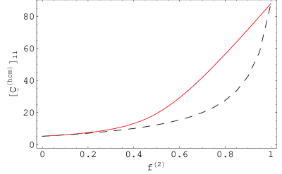
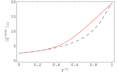
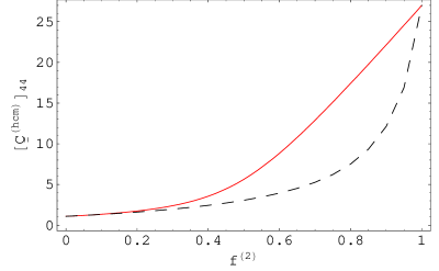
Figure 6: Plots of $\left[\,\underline{\underline{\bf C}}^{(hcm)}\,\right]_{rs}$, with $rs\in\left\{11,12,33,44\right\}$ (in GPa) as estimated using the lowest–order SPFT (i.e., $hcm=ocm$) (red, solid curves) and the Mori–Tanaka mean–field formalism (i.e., $hcm=MT$) (black, dashed curves), against the volume fraction of component material ‘2’. The component materials are distributed as spheres. Their constitutive parameters are specified by (50) and (51), with the orthotropy parameter $\varsigma=0.05$.

The lowest–order SPFT and Mori–Tanaka estimates for the HCM arising from orthotropic component materials characterized by $\varsigma=0.05$ and $\varsigma=0.1$ are presented in Fig. 6 and 7, respectively. As previously, only a representative selection of the entries of $\underline{\underline{\bf C}}^{(hcm)}$ are provided here. The plots for $\varsigma=0$, for which case the HCM is isotropic, are the ones displayed in Fig. 1. In a manner resembling the scenario considered in §3.1, the lowest–order SPFT and the Mori–Tanaka estimates are qualitatively similar, but the Mori–Tanaka estimates display a greater deviation from the naive HCM estimate $f^{(1)}\left[\,\underline{\underline{\bf C}}^{(1)}\,\right]_{pq}+f^{(2)}\left[\,\underline{\underline{\bf C}}^{(2)}\,\right]_{pq}$ for mid–range values of $f^{(2)}$, at all values of $\varsigma$.

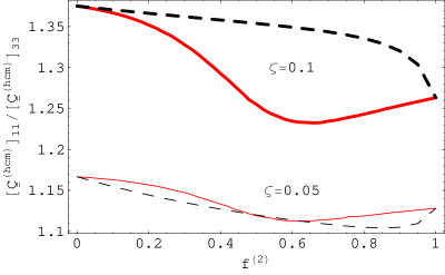
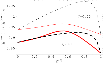
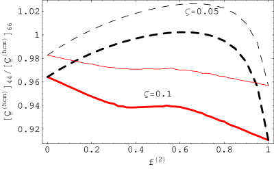
Figure 8: Plot of $\left[\,\underline{\underline{\bf C}}^{(hcm)}\,\right]_{11}/\left[\,\underline{\underline{\bf C}}^{(hcm)}\,\right]_{33}$, $\left[\,\underline{\underline{\bf C}}^{(hcm)}\,\right]_{12}/\left[\,\underline{\underline{\bf C}}^{(hcm)}\,\right]_{23}$ and $\left[\,\underline{\underline{\bf C}}^{(hcm)}\,\right]_{44}/\left[\,\underline{\underline{\bf C}}^{(hcm)}\,\right]_{66}$ (in GPa) as estimated using the lowest–order SPFT (i.e., $hcm=ocm$) (red, solid curves), the Mori–Tanaka mean–field formalism (i.e., $hcm=MT$) (black, dashed curves) against the volume fraction of component material ‘2’. Component material ‘1’ is acetal and component material ‘2’ is glass, as specified in (42). The component materials are distributed as spheres with the orthotropy parameter $\varsigma=0.05$ (thin curves) and $\varsigma=0.1$ (thick curves).

The degree of orthotropy exhibited by the HCM clearly increases as the value of $\varsigma$ increases, and differences between the estimates of the lowest–order SPFT and the Mori–Tanaka mean–field formalism also vary as $\varsigma$ increases. To explore this matter further, in Fig. 8 the associated ratios $\left[\,\underline{\underline{\bf C}}^{(hcm)}\,\right]_{11}/\left[\,\underline{\underline{\bf C}}^{(hcm)}\,\right]_{33}$, $\left[\,\underline{\underline{\bf C}}^{(hcm)}\,\right]_{12}/\left[\,\underline{\underline{\bf C}}^{(hcm)}\,\right]_{23}$ and $\left[\,\underline{\underline{\bf C}}^{(hcm)}\,\right]_{44}/\left[\,\underline{\underline{\bf C}}^{(hcm)}\,\right]_{44}$ are plotted against $f^{(2)}$ for $\varsigma=0.05$ and $0.1$. The three different patterns are portrayed in the three plots: for $\left[\,\underline{\underline{\bf C}}^{(hcm)}\,\right]_{11}/\left[\,\underline{\underline{\bf C}}^{(hcm)}\,\right]_{33}$ differences between the lowest–order SPFT and the Mori–Tanaka estimates are larger for when the HCM is more orthotropic; the reverse is the case for $\left[\,\underline{\underline{\bf C}}^{(hcm)}\,\right]_{12}/\left[\,\underline{\underline{\bf C}}^{(hcm)}\,\right]_{23}$, while for $\left[\,\underline{\underline{\bf C}}^{(hcm)}\,\right]_{44}/\left[\,\underline{\underline{\bf C}}^{(hcm)}\,\right]_{66}$ there is no noticeable difference between the lowest–order SPFT and Mori–Tanaka estimates as the degree of HCM orthotropy is increased.

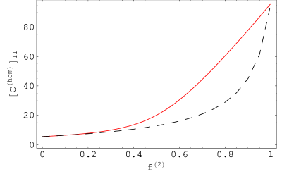
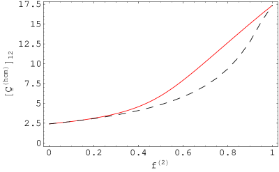
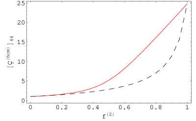
Figure 7: As Fig. 6 but with orthotropy parameter $\varsigma=0.1$.

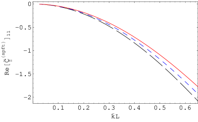
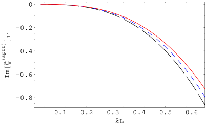
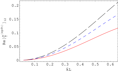
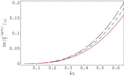
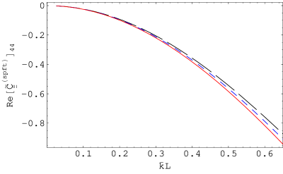
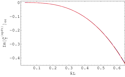
Figure 9: The real and imaginary parts of $\left[\underline{\underline{\bf\tilde{C}}}^{(spft)}\,\right]_{rs}$, with $rs\in\left\{11,12,44\right\}$ (in GPa) plotted as functions of $\bar{k}L$, for $f^{(2)}=0.5$. The component materials are distributed as spheres. Their constitutive parameters are specified by (50) and (51), with the orthotropy parameter $\varsigma=0$ (red, solid curves), $\varsigma=0.05$ (blue, short-dashed curves) and $\varsigma=0.1$ (black, long-dashed curves).

Next we focus on the second–order SPFT estimate of the HCM stiffness tensor. The real and imaginary parts of a representative selection of entries of $\underline{\underline{\bf\tilde{C}}}^{(spft)}=\underline{\underline{\bf C}}^{(spft)}-\underline{\underline{\bf C}}^{(ocm)}$ are graphed against $\bar{k}L$ in Fig. 9. The volume fraction is fixed at $f^{(2)}=0.5$. The values of the orthotropy parameter $\varsigma$ are $0$, $0.05$ and $0.1$, in correspondence with the calculations of Figs. 1, 6 and 7. As we observed in §3.1, the magnitude of the components of $\underline{\underline{\bf\tilde{C}}}^{(spft)}$ generally decrease as the HCM becomes more orthotropic. Also, the second–order SPFT estimate $\underline{\underline{\bf C}}^{(spft)}$ has components with nonzero imaginary parts, which implies that the HCM is effectively dissipative even though the component materials are nondissipative. Furthermore, the HCM becomes increasingly dissipative as the correlation length increases, this effective dissipation being attributable to scattering losses.

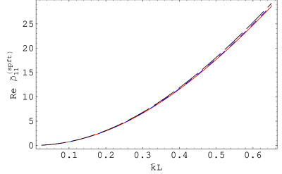
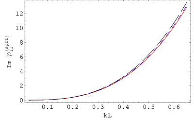
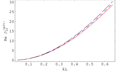
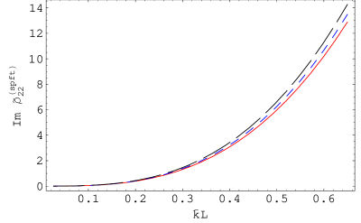
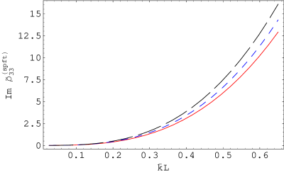
Figure 10: As Fig. 9 but the quantities plotted are the real and imaginary parts of the excess of the second–order SPFT density tensor over the density of the comparison material, i.e., $\tilde{\rho}^{(spft)}_{rr}=\rho^{(spft)}_{rr}-\rho^{(ocm)}$, ($r\in\left\{1,2,3\right\}$), in $\mbox{kg}\,\mbox{m}^{-3}$.

Finally, the real and imaginary parts of the second–order SPFT density tensor $\tilde{\rho}^{(spft)}_{pq}=\rho^{(spft)}_{pq}-\rho^{(ocm)}$ are plotted as functions of $\bar{k}L$ in Fig. 10. As previously in §3.1, the components for $p\neq q$ are negligibly small so only the $p=q$ components are provided here. The density plots resemble those of the corresponding stiffness tensor; i.e., the components $\tilde{\rho}^{(spft)}_{pp}$ are much smaller than $\rho^{(ocm)}$ and they increase rapidly from zero as $L$ increases from zero. The magnitudes of $\tilde{\rho}^{(spft)}_{pp}$ are smallest when the orthotropy parameter describing the component materials is greatest.

4 Closing remarks

The elastodynamic SPFT has been further developed, in order to undertake numerical studies based on a specific choice of two–point covariance function. From our theoretical considerations in §2 and our representative numerical studies in §3, involving generally orthotropic component materials which are distributed as oriented ellipsoids, the following conclusions were drawn:

• The lowest–order SPFT estimate of the HCM stiffness tensor is qualitatively similar to that provided by the Mori–Tanaka mean–field formalism.

• Differences between the estimates of the lowest–order SPFT and the Mori–Tanaka mean–field formalism are greatest for mid–range values of the volume fraction.

• Differences between the estimates of the lowest–order SPFT and the Mori–Tanaka mean–field formalism vary as the HCM becomes more orthotropic. The degree of orthotropy of the HCM may be increased by increasing either the degree of orthotropy of component materials or the degree of eccentricity (nonsphericity) of the component particles.

• The second–order SPFT provides a low–frequency correction to the quasi–static lowest–order estimates of the HCM stiffness tensor and density. The correction vanishes as the correlation length tends to zero.

• The correction provided by second–order SPFT, though relatively small in magnitude, is highly significant as it indicates effective dissipation due to scattering loss.

• Differences between the second–order and lowest–order SPFT estimates of the HCM constitutive parameters diminish as the HCM becomes more orthotropic.

The ability to accommodate higher–order descriptions of the distributional statistics of the component materials bodes well for the future deployment of the SPFT in exploring the complex behaviour of metamaterials as HCMs. Additionally, since the SPFT has been now established for acoustic, electromagnetic and elastodynamic homogenization scenarios, the prospect of considering HCMs with mixed acoustic/elastodynamic/electromagnetic constitutive relations beckons.

Acknowledgements: AJD is supported by an Engineering and Physical Sciences Research Council (UK) studentship. AL thanks the Charles Godfrey Binder Professorship Endowment for partial support.

Appendix A

Matrix/tensor algebra

A fourth–order tensor $A_{rstu}$ ($r,s,t,u\in\left\{1,2,3\right\}$) has $81$ components. If it obeys the symmetries $A_{rstu}=A_{srtu}=A_{rsut}=A_{turs}$, it can be represented by a 9$\times$9 matrix $\underline{\underline{\bf A}}$ with components $\left[\,\underline{\underline{\bf A}}\,\right]_{RS}$ ($R,S\in\left\{1,\ldots,9\right\}$) . Similarly, the nine entries of a second–order tensor $B_{rs}$ ($r,s\in\left\{1,2,3\right\}$) may be expressed as a column 9–vector ${\bf B}$ with components $\left[\,{\bf B}\,\right]_{R}$ ($R\in\left\{1,\ldots,9\right\}$). The scheme for converting between the tensor subscript pairs $rs$ and $tu$ and the matrix indexes $RS$ or vector index $R$ is provided in Table 1.

$R,S$	$rs,tu$	$R,S$	$rs,tu$	$R,S$	$rs,tu$
$1$	$11$	$4$	$23$ or $32$	$7$	$23$ or $32$
$2$	$22$	$5$	$13$ or $31$	$8$	$13$ or $31$
$3$	$33$	$6$	$12$ or $21$	$9$	$12$ or $21$

Table 1: Conversion between tensor and matrix/vector subscripts.

The most general 9$\times$9 matrix $\underline{\underline{\bf A}}$ considered in this paper has the form

$$\underline{\underline{\bf A}}=\left(\begin{array}[]{lll}\underline{\underline{\bf\mbox{\boldmath$\alpha$}}}&\underline{\underline{\bf 0}}&\underline{\underline{\bf 0}}\\ \underline{\underline{\bf 0}}&\underline{\underline{\bf\mbox{\boldmath$\beta$}}}&\underline{\underline{\bf\mbox{\boldmath$\beta$}}}\\ \underline{\underline{\bf 0}}&\underline{\underline{\bf\mbox{\boldmath$\beta$}}}&\underline{\underline{\bf\mbox{\boldmath$\beta$}}}\end{array}\right),$$ (52)

where $\underline{\underline{\bf\mbox{\boldmath$\alpha$}}}$ is a general 3$\times$3 matrix, $\underline{\underline{\bf\mbox{\boldmath$\beta$}}}$ is a diagonal 3$\times$3 matrix, and $\underline{\underline{\bf 0}}$ is the null 3$\times$3 matrix. If we define a 9$\times$9 matrix $\underline{\underline{\bf A}}^{\dagger}$ as [36]

$$\underline{\underline{\bf A}}^{\dagger}=\left(\begin{array}[]{lll}\underline{\underline{\bf\mbox{\boldmath$\alpha$}}}^{-1}&\underline{\underline{\bf 0}}&\underline{\underline{\bf 0}}\vspace{4pt}\\ \underline{\underline{\bf 0}}&\frac{1}{4}\,\underline{\underline{\bf\mbox{\boldmath$\beta$}}}^{-1}&\frac{1}{4}\,\underline{\underline{\bf\mbox{\boldmath$\beta$}}}^{-1}\vspace{4pt}\\ \underline{\underline{\bf 0}}&\frac{1}{4}\,\underline{\underline{\bf\mbox{\boldmath$\beta$}}}^{-1}&\frac{1}{4}\,\underline{\underline{\bf\mbox{\boldmath$\beta$}}}^{-1}\end{array}\right),$$ (53)

then $\underline{\underline{\bf A}}^{\dagger}\cdot\underline{\underline{\bf A}}=\underline{\underline{\bf A}}\cdot\underline{\underline{\bf A}}^{\dagger}=\underline{\underline{\bf\mbox{\boldmath$\tau$}}}$, where $\underline{\underline{\bf\mbox{\boldmath$\tau$}}}$ is the 9$\times$9 matrix counterpart of the identity tensor

$$\tau_{rstu}=\frac{1}{2}\left(\delta_{rt}\delta_{su}+\delta_{ru}\delta_{st}\right).$$ (54)

Appendix B

Eshelby matrix/tensor

If the component materials are orthotropic and distributed as spherical particles (i.e., $a=b=c$), then the tensor counterpart of the 9$\times$9 Eshelby matrix is given as [58]

$$S^{(esh)}_{ijkl}=\frac{1}{8\pi}C^{(1)}_{mnkl}\int_{-1}^{+1}d\zeta_{3}\int_{0}^{2\pi}d\omega\;\left[\,F_{imjn}(\overline{\vartheta})+F_{jmin}(\overline{\vartheta})\,\right],$$ (55)

wherein

$$\left.\begin{array}[]{l}\displaystyle{F_{ijkl}(\overline{\vartheta})=\frac{\overline{\vartheta}_{k}\overline{\vartheta}_{l}N_{ij}}{D},\qquad N_{ij}(\overline{\vartheta})=\frac{1}{2}\epsilon_{ikl}\epsilon_{jmn}K_{km}K_{ln}\vspace{4pt}}\\ \displaystyle{D=\epsilon_{mnl}K_{m1}K_{n2}K_{l3},\qquad K_{ik}=C^{(1)}_{ijkl}\overline{\vartheta}_{j}\overline{\vartheta}_{l}}\\ \displaystyle{\overline{\vartheta}_{1}=\frac{\zeta_{1}}{a},\qquad\overline{\vartheta}_{2}=\frac{\zeta_{2}}{b},\qquad\overline{\vartheta}_{3}=\frac{\zeta_{3}}{c}\vspace{4pt}}\\ \displaystyle{\zeta_{1}=(1-\zeta_{3}^{2})^{1/2}\cos(\omega),\qquad\zeta_{2}=(1-\zeta_{3}^{2})^{1/2}\sin(\omega),\qquad\zeta_{3}=\zeta_{3}}\end{array}\right\},$$ (56)

with $\epsilon_{ijk}$ being the Levi–Civita symbol. The integrals in (55) can be evaluated using standard numerical methods [47].

If the component materials are isotropic and distributed as ellipsoidal particles described by the shape matrix $\underline{\underline{\bf U}}$, then the Eshelby matrix has the form represented in (52) with distinct components given as [51]

$$\left[\,\underline{\underline{\bf S}}^{(esh)}\,\right]_{11} = \frac{3a^{2}I_{\alpha\alpha}+\left(1-2\nu^{(1)}\right)I_{\alpha}}{8\pi\left(1-\nu^{(1)}\right)},$$ (57)

$$\left[\,\underline{\underline{\bf S}}^{(esh)}\,\right]_{12} = \frac{3b^{2}I_{\alpha\beta}-\left(1-2\nu^{(1)}\right)I_{\alpha}}{8\pi\left(1-\nu^{(1)}\right)},$$ (58)

$$\left[\,\underline{\underline{\bf S}}^{(esh)}\,\right]_{13} = \frac{3c^{2}I_{\alpha\gamma}-\left(1-2\nu^{(1)}\right)I_{\alpha}}{8\pi\left(1-\nu^{(1)}\right)},$$ (59)

$$\left[\,\underline{\underline{\bf S}}^{(esh)}\,\right]_{21} = \frac{3a^{2}I_{\alpha\beta}-\left(1-2\nu^{(1)}\right)I_{\beta}}{8\pi\left(1-\nu^{(1)}\right)},$$ (60)

$$\left[\,\underline{\underline{\bf S}}^{(esh)}\,\right]_{22} = \frac{3b^{2}I_{\beta\beta}+\left(1-2\nu^{(1)}\right)I_{\beta}}{8\pi\left(1-\nu^{(1)}\right)},$$ (61)

$$\left[\,\underline{\underline{\bf S}}^{(esh)}\,\right]_{23} = \frac{3c^{2}I_{\beta\gamma}+\left(1-2\nu^{(1)}\right)I_{\beta}}{8\pi\left(1-\nu^{(1)}\right)},$$ (62)

$$\left[\,\underline{\underline{\bf S}}^{(esh)}\,\right]_{31} = \frac{3a^{2}I_{\alpha\gamma}-\left(1-2\nu^{(1)}\right)I_{\gamma}}{8\pi\left(1-\nu^{(1)}\right)},$$ (63)

$$\left[\,\underline{\underline{\bf S}}^{(esh)}\,\right]_{32} = \frac{3b^{2}I_{\beta\gamma}-\left(1-2\nu^{(1)}\right)I_{\gamma}}{8\pi\left(1-\nu^{(1)}\right)},$$ (64)

$$\left[\,\underline{\underline{\bf S}}^{(esh)}\,\right]_{33} = \frac{3c^{2}I_{\gamma\gamma}+\left(1-2\nu^{(1)}\right)I_{\gamma}}{8\pi\left(1-\nu^{(1)}\right)},$$ (65)

$$\left[\,\underline{\underline{\bf S}}^{(esh)}\,\right]_{44} = \frac{3(b^{2}+c^{2})I_{\beta\gamma}+\left(1-2\nu^{(1)}\right)(I_{\beta}+I_{\gamma})}{16\pi\left(1-\nu^{(1)}\right)},$$ (66)

$$\left[\,\underline{\underline{\bf S}}^{(esh)}\,\right]_{55} = \frac{3(a^{2}+c^{2})I_{\alpha\gamma}+\left(1-2\nu^{(1)}\right)(I_{\alpha}+I_{\gamma})}{16\pi\left(1-\nu^{(1)}\right)},$$ (67)

$$\left[\,\underline{\underline{\bf S}}^{(esh)}\,\right]_{66} = \frac{3(a^{2}+b^{2})I_{\alpha\beta}+\left(1-2\nu^{(1)}\right)(I_{\alpha}+I_{\beta})}{16\pi\left(1-\nu^{(1)}\right)},$$ (68)

where $\nu^{(1)}=\displaystyle{\frac{\lambda^{(1)}}{2\left(\lambda^{(1)}+\mu^{(1)}\right)}}$ is the Poisson ratio of component material ‘1’. For the case $a>b>c$ we have

$$\left.\begin{array}[]{l}I_{\alpha}=\displaystyle{\frac{4\pi abc}{(a^{2}-b^{2})(a^{2}-c^{2})^{1/2}}\left[\,F(\tilde{\theta},\tilde{k})-E(\tilde{\theta},\tilde{k})\right]\vspace{4pt}}\\ I_{\gamma}=\displaystyle{\frac{4\pi abc}{(b^{2}-c^{2})(a^{2}-c^{2})^{1/2}}\left[\,\frac{b}{ac}(a^{2}-c^{2})^{1/2}-E(\tilde{\theta},\tilde{k})\right]\vspace{4pt}}\\ I_{\beta}=\displaystyle{4\pi-(I_{\alpha}+I_{\gamma})},\qquad I_{\alpha\beta}=\displaystyle{\frac{I_{\alpha}-I_{\beta}}{3(b^{2}-a^{2})}},\qquad I_{\alpha\gamma}=\displaystyle{\frac{I_{\alpha}-I_{\gamma}}{3(c^{2}-a^{2})}},\qquad I_{\beta\gamma}=\displaystyle{\frac{I_{\beta}-I_{\gamma}}{3(c^{2}-b^{2})}\vspace{4pt}}\\ I_{\alpha\alpha}=\displaystyle{\frac{4\pi}{3a^{2}}-(I_{\alpha\beta}+I_{\alpha\beta})},\qquad I_{\beta\beta}=\frac{4\pi}{3b^{2}}-(I_{\alpha\beta}+I_{\beta\gamma}),\qquad I_{\gamma\gamma}=\frac{4\pi}{3c^{2}}-(I_{\alpha\gamma}+I_{\beta\gamma})\end{array}\right\},$$ (69)

with the elliptic integrals given by

$$\left.\begin{array}[]{l}\displaystyle{E(\tilde{\theta},\tilde{k})=\int_{0}^{\tilde{\theta}}d\phi\;(1-\tilde{k}^{2}\sin^{2}\phi)^{1/2}\vspace{4pt}}\\ \displaystyle{F(\tilde{\theta},\tilde{k})=\int_{0}^{\tilde{\theta}}d\phi(1-\tilde{k}^{2}\sin^{2}\phi)^{-1/2}}\end{array}\right\},$$ (70)

wherein

$$\tilde{\theta}=\sin^{-1}\frac{(a^{2}-c^{2})^{1/2}}{a},\qquad\tilde{k}=\frac{(a^{2}-b^{2})^{1/2}}{(a^{2}-c^{2})^{1/2}}.$$ (71)

References

- [1] Lakhtakia, A. (Ed.), (1996) Selected Papers on Linear Optical Composite Materials. Bellingham, WA, USA: SPIE.
- [2] Milton, G.W. (2002) The Theory of Composites. Cambridge, UK: Cambridge University Press.
- [3] Walser, R.M. (2003) Metamaterials: an introduction. Introduction to Complex Mediums for Optics and Electromagnetics (W.S. Weiglhofer, A. Lakhtakia eds.). Bellingham, WA, USA: SPIE, pp. 295–316.
- [4] Mei, J., Liu, Z., Wen, W. & Sheng, P. (2007) Effective dynamic mass density of composites. Phys. Rev. B, 76, 134205.
- [5] Lakes, R.S. (2001) Extreme damping in composite materials with a negative stiffness phase. Phys. Rev. Lett., 86, 2897–2900.
- [6] Fang, N., Xi, D., Xu, J., Ambati, M., Srituravanich, W., Sun, C. & Zhang Y. (2006) Ultrasonic metamaterials with negative modulus. Nature Materials, 5, 452–456.
- [7] Ramakrishna, S.A. (2005) Physics of negative refractive index materials. Rep. Prog. Phys., 68, 449–521.
- [8] Ryzhov, Yu A. & Tamoikin, V.V. (1970) Radiation and propagation of electromagnetic waves in randomly inhomogeneous media. Radiophys. Quantum Electron., 14, 228–233.
- [9] Hill R. (1963) A self–consistent mechanics of composite materials. J. Mech. Phys. Solids, 13, 213–222.
- [10] Hill R. (1965) Elastic properties of reinforced solids: some theoretical principles. J. Mech. Phys. Solids, 11, 357–372.
- [11] Budiansky B. (1965) On the elastic moduli of some heterogeneous materials. J. Mech. Phys. Solids, 13, 223–227.
- [12] Sabina, F.J. & Willis, J.R. (1988) A simple self-consistent analysis of wave propagation in particulate composites. Wave Motion, 10, 127–142.
- [13] Kim, J.–Y. (2004) On the generalized self–consistent model for elastic wave propagation in composite materials. Int. J. Solids Structures, 41, 4349–4360.
- [14] Kanaun, S.K. & Levin, V.M. (2005) Propagation of shear elastic waves in composites with a random set of spherical inclusions (effective field approach). Int. J. Solids Structures, 42, 3971–3997.
- [15] Wang, Y. & Qin, Q.–H. (2007) A generalized self consistent model for effective elastic moduli of human dentine. Compos. Sci. Technol., 67, 1553–1560.
- [16] Twersky, V. (1962) On scattering of waves by random distributions. I. Free–space scatterer formalism. J. Math. Phys., 3, 700–715.
- [17] Linton, C.M. & Martin, P.A. (2006) Multiple scattering by multiple spheres: a new proof of the Lloyd–Berry formula for the effective wavenumber. SIAM J. Appl. Math., 66, 1649–1668.
- [18] Ávila–Carrera, R., Sánchez–Sesma, F.J. & Avilés, J. (2008) Transient response and multiple scattering of elastic waves by a linear array of regulaly distributed cylindrical obstacles: Anti–plane S–wave analytical solution. Geofís. Int., 47, 115–126.
- [19] Datta, S.K. & Ledbetter, H.M. (1986) Effective wave speeds in an SiC–particle–reinforced Al composite. J. Acoust. Soc. Am., 79, 239–248.
- [20] Varadan, V.K., Ma, Y. & Varadan, V.V. (1989) Scattering and attenuation of elastic waves in random media. Pure Appl. Geophys., 131, 577–603.
- [21] Maurel, A., Mercier, J.–F. & Lund, F. (2004) Elastic wave propagation through a random array of dislocations. Phys. Rev. B, 70, 024303.
- [22] Hashin, Z. & Shtrikman, S. (1962) On some variational principles in anisotropic and nonhomogeneous elasticity. J. Mech. Phys. Solids, 10, 335–342.
- [23] Kröner, E. (1977) Bounds for the effective elastic moduli of disordered materials. J. Mech. Phys. Solids, 25, 137–155.
- [24] Willis, J.R. (1981) Variational and related methods for the overall properties of composites. Advances in Applied Mechanics (ed. C.S. Jeh ed.), vol. 21. New York, NY, USA: Academic, pp.1–79.
- [25] Talbot, D.R.S. & Willis, J.R. (1982) Variational estimates for the dispersion and attenuation of waves in random composites I. General theory. Int. J. Solids Structures, 18, 673–683.
- [26] Hashin, Z. (1983) Analysis of composite materials — a survey. J. Appl. Mech., 50, 481–505.
- [27] Tsang, L. & Kong, J.A. (1981) Scattering of electromagnetic waves from random media with strong permittivity fluctuations. Radio Sci., 16, 303–320.
- [28] Genchev, Z.D. (1992) Anisotropic and gyrotropic version of Polder and van Santen’s mixing formula. Waves Random Media, 2, 99–110.
- [29] Michel, B. & Lakhtakia, A. (1995) Strong–property–fluctuation theory for homogenizing chiral particulate composites. Phys. Rev. E, 51, 5701–5707.
- [30] Mackay, T.G., Lakhtakia, A. & Weiglhofer, W.S. (2000) Strong-property-fluctuation theory for homgenization of bianisotropic composites: Formulation. Phys. Rev. E, 62, 6052–6064. Erratum: (2001) 63, 049901.
- [31] Cui, J. & Mackay, T.G. (2007) Depolarization regions of nonzero volume in bianisotropic homogenized composites. Waves Random Complex Media, 17, 269–281.
- [32] Zhuck, N.P. (1996) Strong fluctuation theory for a mean acoustic field in a random fluid medium with statistically anisotropic perturbations. J. Acoust. Soc. Am., 99, 46–54.
- [33] Zhuck, N.P. & Lakhtakia, A. (1999) Effective constitutive properties of a disordered elastic solid medium via the strong-fluctuation approach. Proc R. Soc. Lond. A, 455, 543–566.
- [34] Mori, T. & Tanaka, K. (1993) Average stress in matrix and average elastic energy of materials misfitting inclusions. Acta Metallurgica, 21, 571–574.
- [35] Benveniste, Y. (1987) A new approach to the application of Mori-Tanaka’s theory in composite materials. Mech. Materials 6, 147–157.
- [36] Lakhtakia, A. (2002) Microscopic model for elastostatic and elastodynamic excitation of chiral sculptured thin films. J. Compos. Mater., 36, 1277–1298.
- [37] Lakhtakia, A. (1996) Introduction Selected Papers on Linear Optical Composite Materials (A. Lakhtakia ed.). Bellingham, WA, USA: SPIE.
- [38] Mackay, T.G. (2008) Lewin’s homogenization formula revisited for nanocomposite materials. J. Nanophoton., 2, 029503.
- [39] Červený, V. & Pšenčik, I. (2006) Energy flux in viscolelastic anisotropic media. Geophys. J. Int., 166, 1299–1317.
- [40] Ting, T.C.T (1996) Anisotropic Elasticity. New York, NY, USA: Oxford University Press.
- [41] Tsang, L, Kong, J.A. & Newton, R.W. (1982) Application of strong fluctuation random medium theory to scattering of electromagnetic waves from a half–space of dielectric mixture. IEEE Trans. Antennas Propagat., 30, 292–302.
- [42] Mackay, T.G., Lakhtakia, A. & Weiglhofer, W.S. (2001) Homogenisation of similarly oriented, metallic, ellipsoidal inclusions using the bilocally approximated strong–property–fluctuation theory. Opt. Commun., 107, 89–95.
- [43] Narasimhan, M.N.L. (1993) Principles of Continuum Mechanics. New York, NY, USA: Wiley.
- [44] Parnell, W.J. & Abrahams, I.D. (2008) Homogenization for wave propagation in periodic fibre–reinforced media with complex microstructure. I–Theory. J. Mech. Phys. Solids, 56, 2521–2540.
- [45] Bagnara R. (1995) A unified proof for the convergence of Jacobi and Gauss–Seidel methods. SIAM Review, 37, 93–97.
- [46] Kwok, Y.K. (2002) Applied Complex Variables for Scientists and Engineers. Cambridge, UK: Cambridge University Press.
- [47] Press, W.H., Flannery, B.P., Teukolsky, S.A. & Vetterling, W.T. (1992) Numerical Recipes in Fortran, 2nd. edition. Cambridge, UK: Cambridge University Press.
- [48] Biwa, S., Kobayashi, F. & Ohno, N. (2007) Influence of disordered fiber arrangement on SH wave transmission in unidirectional composites. Mech. Mater., 39, 1–10.
- [49] Willis, J.R. (1985) The nonlocal influence of density variations in a composite. Int. J. Solids Structures, 21, 805–817.
- [50] Milton, G.W. (2007) New metamaterials with macroscopic behavior outside that of continuum elastodynamics. New J. Physics, 9, 359.
- [51] Mura, T. (1987) Micromechanics of Defects in Solids. Dordrecht, The Netherlands: Martinus Nijhoff Publishers.
- [52] Ferrari, M. & Filipponi, M. (1991) Appraisal of current homogenizing techniques for the elastic response of porous and reinforced glass. J. Am. Ceramic Soc., 74, 229–231.
- [53] Hu, G.K. & Weng, G.J. (2000) Some reflections on the Mori–Tanaka and Ponte Castañeda–Willis methods with randomly oriented ellipsoidal inclusions. Acta Mechanica, 140, 31–40.
- [54] Mercier, S. & Molinari, A. (2008) Homogenization of elastic–viscoelastic heterogeneous materials: Self–consistent and Mori–Tanaka schemes. Int. J. Plasticity, (in press). [doi:10.1016/j.ijplas.2008.08.006]
- [55] Eshelby, J.D. (1957) The determination of the elastic field of an ellipsoidal inclusion, and related problems. Proc. R. Soc. Lond. A, 241, 376–396.
- [56] James, A.M. & Lord, M.P. (1992) MacMillan’s Chemical and Physical Data. London, UK: MacMillan Press.
- [57] Shackelford, J.F. (2005) Introduction to Materials Science for Engineers, 6th. edition. Upper Saddle River, NJ, USA: Pearson Prentice Hall.
- [58] Gavazzi, A.C. & Lagoudas, D.C. (1990) On the numerical evaluation of Eshelby’s tensor and its application to elastoplastic fibrous composites. Comp. Mech., 7, 13–19.