A Simple Statistical Mechanical Approach for Studying Multilayer Adsorption of Interacting Polyatomics
Abstract
A simple statistical mechanical approach for studying multilayer adsorption of interacting polyatomic adsorbates (-mers) has been presented. The new theoretical framework has been developed on a generalization in the spirit of the lattice-gas model and the classical Bragg-Williams (BWA) and quasi-chemical (QCA) approximations. The derivation of the equilibrium equations allows the extension of the well-known Brunauer-Emmet-Teller (BET) isotherm to more complex systems. The formalism reproduces the classical theory for monomers, leads to the exact statistical thermodynamics of interacting -mers adsorbed in one dimension, and provides a close approximation for two-dimensional systems accounting multisite occupancy and lateral interactions in the first layer. Comparisons between analytical data and Monte Carlo simulations were performed in order to test the validity of the theoretical model. The study showed that: the resulting thermodynamic description obtained from QCA is significantly better than that obtained from BWA and still mathematically handable; for non-interacting -mers, the BET equation leads to an underestimate of the true monolayer volume; attractive lateral interactions compensate the effect of the multisite occupancy and the monolayer volume predicted by BET equation agrees very well with the corresponding true value; and repulsive couplings between the admolecules hamper the formation of the monolayer and the BET results are not good (even worse than those obtained in the non-interacting case).
keywords:
Equilibrium thermodynamics and statistical mechanics , Surface thermodynamics , Adsorption isotherms , Monte Carlo simulations, , ,
1 Introduction
Adsorption on solid surfaces is a complex phenomenon [1, 2, 3, 4, 5], which implies a series of questions about the nature of the forces binding foreign molecules to a surface and about the thermodynamic behavior of the system. Although the problem of the forces is still far from being elucidated, a large amount of interest has been devoted to the study of statistical properties, within the frame of simplified models for both monolayer and multilayer adsorption. In 1918 Langmuir derived the monolayer adsorption isotherm kinetically for gas molecules adsorbed on the homogeneous surface of adsorbents without attractions among the adsorbed molecules [6]. After that Brunauer, Emmett and Teller [7], based on a model of localized adsorption, developed the most important theory of multilayer adsorption. Their equation, the BET isotherm, was the first and the most useful, covering the complete range of pressures up to , the saturation pressure. Later, Hill [1] derived the BET isotherm statistically on a group of homogeneous adsorption sites for the multilayer adsorption since it was derived kinetically by Brunauer, Emmett and Teller. It is found to be in good agreement with some experimental data for relative pressures less than about [8].
But the theoretical BET isotherm deals with the common assumption that each ad-molecule occupies one adsorption site of the surface. However, most adsorbates involved in experiments are polyatomic; hence, the theoretical description of their thermodynamic properties is a topic of much interest in adsorption theory111Even for simple gases such as oxygen, nitrogen and carbon monoxide, which basically are not altered in their molecular dimensions under physical adsorption, the adsorption energy depends in general on the orientation of the molecule in the adsorbed state.. Leading contributions to this subject, generically called multisite-occupancy adsorption, have been presented by Flory [9], Huggins [10], Guggenheim [11], DiMarzio [12], Nitta et al. [13] and Rudzinski et al. [14] through approximate treatments of monolayer adsorption on homogeneous and heterogeneous surfaces. More recently, Aranovich and Donohue [15, 16] derived a multilayer adsorption isotherm, which is not limited by the functional form of the monolayer adsorption isotherm and should be capable to include multisite occupancy (with an adequate choice of a fitting parameter). On the other hand, the closed exact solution for the multilayer adsorption isotherm of dimers, along with the basis for calculating adsorption thermodynamics of homonuclear polyatomic molecules (-mers) on one-(1D) and two-dimensional (2D) substrates, have been recently presented [17, 18]. This rigorous thermodynamic study demonstrated that the entropic contribution of non-spherical adsorbates is significant in the multilayer regime when compared with monoatomic adsorption. Thus, the determinations of surface areas and adsorption energies from polyatomic adsorbate adsorption may be severely misestimated, if this polyatomic character is not properly incorporated in the thermodynamic functions from which experiments are interpreted.
There is another important physical fact which has not been sufficiently studied; namely, the effect of the lateral interactions between the ad-molecules in presence of multilayer adsorption and multisite occupancy. Thus, most of the theoretical work dealing with adsorption of interacting polyatomics has been based on models of monolayer adsorption. In this context, the aim of the present work is to extend the treatment of Refs. [17, 18] to include lateral interactions in the adsorbate. Here, we introduce nearest-neighbor interactions between the molecules adsorbed in the first layer222 As it is well-known, BET equation can be applied at coverage not greatly exceeding (statistically) monolayer coverage. Thus, although the contribution from the secondary adsorption can already be significant, the density of the molecules in the second and higher adlayers is expected to be much lower than that in the first adsorbed layer. Therefore, it seems to be satisfactorily enough to take into account only the interactions between the primarily adsorbed molecules [1]., by following the configuration-counting procedure of the Bragg-Williams approach and the quasi-chemical approximation. In addition, Monte Carlo (MC) simulations are performed in order to test the validity of the theoretical model. The new theoretical scheme allows us: (1) to reproduce the classical theory for monomers [1, 5]; (2) to develop a closed exact expression for the multilayer adsorption isotherm of interacting -mers on 1D chains; (3) to obtain an accurate approximation for multilayer adsorption on 2D substrates accounting multisite occupancy and lateral interactions; and (4) to provide a simple model from which experiments may be reinterpreted.
The present work is organized as follows. In Section 2, the theoretical formalism along with the basis of the MC method are presented. In Section 3, the results of the theoretical model are shown and discussed by comparing with MC simulations. Finally, conclusions are drawn in Section 4.
2 Basic Definitions: Adsorption Model and Monte Carlo Simulation
2.1 Model
In this section we present the lattice-gas model for the adsorption of particles with multisite occupancy in the multilayer regime. The adsorbent is a homogeneous lattice of sites with coordination number . The adsorbate is assumed as linear molecules having -identical units (-mers) each of which occupies an adsorption site. Furthermore, i) a -mer can adsorb exactly onto an already adsorbed one; ii) attractive and repulsive lateral interactions are considered in the first layer and horizontal interactions are ignored in higher layers; iii) the adsorption heat in all layers, except the first one, equals the molar heat of condensation of the adsorbate in bulk liquid phase. Thus, with denotes the ratio between the single-molecule partition functions in the first and higher layers [17]. The fact that -mers can arrange in the first layer leaving sequences of empty sites with , where no further adsorption of a mer can occur in such a configuration, makes the calculation of entropy much elaborated than the one for monomer adsorption.
To describe a system of -mers adsorbed on sites at a given temperature , let us introduce the occupation variable which can take the values or , if the site is empty or occupied by a -mer unit, respectively. Under these conditions, the Hamiltonian of the system is given by
| (1) |
where () represents the adsorption energy of a -mer unit on the first layer (higher layers); is the number of -mers adsorbed on the first layer; is the lateral interaction energy between two nearest-neighbor (NN) units belonging to different -mers adsorbed in the first layer (we use for repulsive and for attractive interactions) and represents pairs of NN sites. The term is subtracted in equation (1) since the summation over all the pairs of NN sites overestimates the total energy by including bonds belonging to the adsorbed -mers.
2.2 Theory
From a theoretical point of view, when intermolecular forces are introduced (in our case, NN interactions in the first layer), an extra term in the partition function for interaction energy is required. With this extra term, only partition functions for the whole system can be written. Ising [19] gave an exact solution to the 1D monolayer in 1925. All other cases are expressed in terms of series solution [1, 20], except for the special case of 2D monolayers at half-coverage, which was exactly solved by Onsager [21] in 1944. Close approximate solutions in dimensions higher than one can be obtained, and the two most important of these are the Bragg-Williams approximation (BWA) [1] and the quasi-chemical approximation (QCA) [1, 22]. These leading models have played a central role in the study of adsorption systems in presence of lateral interactions between the adatoms. Next, we apply BWA and QCA to study multilayer adsorption of interacting -mers.
The BWA is the simplest mean-field treatment for interacting adsorbed particles, even in the case of multilayer adsorption and multisite occupancy. For a lattice having adsorption sites, the maximum number of columns that can be grown up onto it is . If an infinite number of layers is allowed to develop on the surface, the grand partition function, , of the adlayer in equilibrium with a gas phase at chemical potential and temperature , is given by
| (2) |
where is the grand partition function of a single column of -mers having at least one -mer in the first layer; is the total number of distinguishable configurations of columns on sites with connectivity and is the mean total energy of the system assuming that the columns are randomly distributed over the lattice.
Then,
| (3) |
where is the fugacity and is the Boltzmann constant. In addition, it is possible to demonstrate that is the relative pressure [5, 17].
can be approximated considering that the columns are distributed completely at random on the lattice and assuming the arguments given by different authors [23, 24, 25] to relate the configurational factor for any , with the same quantity in the 1D case . Thus
| (4) |
where is, in general, a function of the connectivity and the size of the molecules. In the particular case of rigid straight -mers it follows that . In addition, can be readily calculated [25] giving
| (5) |
On the other hand, needs to be calculated. For this purpose, let us consider the number of NN of a -mer (column) adsorbed in the first layer,
| (6) |
where the first term in the RHS of Eq. (6) is the number of NN connected to both extrems of the -mer and the second term is due to the NN connected to the inner units of the molecule. The probability that one of the NN is filled by molecules is equal to (random distribution of molecules among sites). Then, the mean number of pairs of filled sites is given by
| (7) | |||||
Then, the grand partition function can be written as,
| (8) |
When , the summation in Eq. (8) can be performed very easily. In the more general case , the summation cannot be done in an easy way, but we can apply the method of the maximum term. Then, the sum in Eq. (8) is replaced by its maximum term, found from the condition , being . Thus,
| (9) |
where is the value of giving the maximum term in the sum in Eq. (8).
Introducing in Eq. (8) and applying Stirling’s approximation, is given by
| (10) | |||||
The average number of the molecules in the adsorption system is
| (11) |
Then,
| (12) | |||||
where and has the following explicit form:
| (13) |
Considering now Eqs. (9), (11), (13) and (14), the adsorption isotherm equation can be obtained. In the case of adsorbed monomers (), Eq. (9) can be written as
| (15) |
and
| (16) |
where is the monolayer coverage, being the total coverage. Then, from Eqs. (3), (11), (13) and (16)
| (17) | |||||
which can be easily recognized as the classical BET equation if we write it in the form
| (18) |
where .
Using Eqs. (3), (11), (13) and (20) we obtain
| (21) | |||||
and, in terms of and ,
| (22) |
Eq. (22) is similar to the recently reported multilayer isotherm for non-interacting dimers [18]. In this case, taking into account the lateral interactions between the primarily adsorbed molecules adds to the adsorption energy the term , which represents the potential of the average force acting on an admolecule in the first adsorbed layer from its NN in the first layer.
For the explicit expression of the adsorption isotherm cannot be obtained in a easy way. However, the calculations for large molecules can be easily done through a standard computing procedure; in our case, we used Maple software.
An alternative method to calculate the multilayer adsorption isotherm was recently reported in Ref.[18]. The theoretical procedure can be described as follows:
-
1)
By using as a parameter (), the relative pressure is obtained by using the condition
(23) where is the monolayer fugacity. This calculation requires the knowledge of an analytical expression for the monolayer adsorption isotherm, .
-
2)
The values of and are introduced in
(24) and the total coverage is obtained.
The equivalence between both methodologies can be easily understood. In fact, Eq. (23) can be obtained from Eq. (3) and the maximum term condition Eq. (9). On the other hand, from Eqs. (11), (13) and (14) and after some algebra, the total coverage can be written in terms of the monolayer coverage, and Eq. (24) is recovered. As an example, in the following we show the use of the method in Ref.[18] to calculate the adsorption isotherms in Eqs. (18) and (22).
We start from the equation
| (25) |
which represents the BWA isotherm of interacting -mers adsorbed at monolayer [26, 27].
Substituting Eq. (25) into Eq. (23), one obtains the following expression for the relative pressure,
| (26) |
Eqs. (24) and (26) represent the mean-field solution describing the adsorption of interacting -mers at multilayer regime on a homogeneous surface. In the case of monomer [dimer] adsorption, Eqs. (24) and (26) reduce to Eq. (18) [(22)].
We now turn to the QCA, which is significantly better than the BWA. The important assumption in this method is that pairs of NN sites are treated as if they were independent of each other (this assumption is, of course, not true, because the pairs overlap [1]).
2.3 Monte Carlo Simulation of Adsorption in the Grand Canonical Ensemble
The adsorption process is simulated through a grand canonical ensemble Monte Carlo (GCEMC) method[18].
For a given value of the temperature and chemical potential , an initial configuration with -mers adsorbed at random positions (on sites) is generated. Then, an adsorption-desorption process is started, where each elementary step is attempted with a probability given by the Metropolis [28] rule:
| (32) |
where and represent the difference between the Hamiltonians and the variation in the number of particles, respectively, when the system changes from an initial state to a final state. In the process there are four elementary ways to perform a change of the system state, namely, adsorbing one molecule onto the surface, desorbing one molecule from the surface, adsorbing one molecule in the bulk liquid phase and desorbing one molecule from the bulk liquid phase. In all cases, .
The algorithm to carry out one MC step (MCS), is the following :
-
1)
Set the value of the chemical potential and the temperature .
-
2)
Set an initial state by adsorbing molecules in the system. Each -mer can adsorb in two different ways: on a linear array of () empty sites on the surface or exactly onto an already adsorbed -mer.
-
3)
Introduce an array, denoted as , storing the coordinates of entities, being ,
(33) where is the sum of two terms: the number of -uples of empty sites on the surface and the number of columns of adsorbed -mers333Note that the top of each column is an available -uple for the adsorption of one -mer..
-
4)
Choose randomly one of the entities, and generate a random number
-
4.1)
if the selected entity is a -uple of empty sites on the surface then adsorb a -mer if , being the transition probability of adsorbing one molecule onto the surface.
-
4.2)
if the selected entity is a -uple of empty sites on the top of a column of height , then adsorb a new -mer in the layer if , being the transition probability of adsorbing one molecule in the bulk liquid phase.
-
4.3)
if the selected entity is a -mer on the surface then desorb the -mer if , being the transition probability of desorbing one molecule from the surface.
-
4.4)
if the selected entity is a -mer on the top of a column then desorb the -mer if , being the transition probability of desorbing one molecule from the bulk liquid phase.
-
4.1)
-
5)
If an adsorption (desorption) is accepted in , then, the array is updated.
-
6)
Repeat from step times.
In the present case, the equilibrium state could be well reproduced after discarding the first . Then, averages were taken over successive configurations. The total coverage was obtained as simple averages,
| (34) |
where is the mean number of adsorbed particles, and means the time average over the MC simulation runs.
The computational simulations have been developed for 1D chains of sites, and square lattices, with , and periodic boundary conditions. With this lattice sizes we verified that finite-size effects are negligible.
3 Results
In the present section, we will analyze the main characteristics of the thermodynamic functions given in Subsection 2.2, in comparison with simulation results for a lattice-gas of interacting -mers on 1D and 2D substrates.
3.1 Exact solution in the 1D case
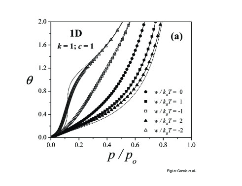
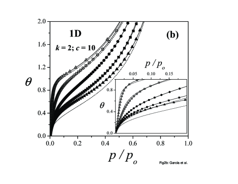
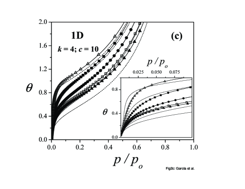
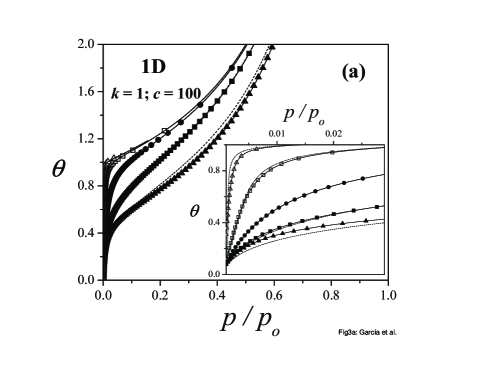
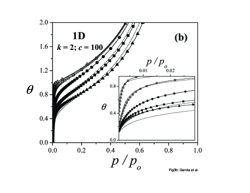
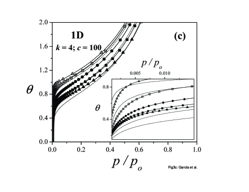
In Figs. 1-3 we address the comparison between the analytical adsorption isotherms for 1D substrates and MC simulations. Different values of the parameter , the lateral interactions and the -mer sizes have been considered.
We start analyzing the case of , and different values of and [see Fig. 1 (a)]. The case (standard BET model) has been widely discussed in the literature (see, for instance, Ref. [8]) and it has been shown that a shape of a Type II isotherm is obtained so long as exceeds 2. In the case of this figure, and the curve for non-interacting particles has the general shape of a Type III isotherm. For repulsive couplings, the interactions do not favor the adsorption on the first layer and the isotherms shift to higher values of pressure. On the other hand, attractive lateral interactions facilitate the formation of the monolayer. Consequently, the isotherms shift to lower values of and their slope increases as the ratio increases. With respect to the shape of the curves, there exists a range of where the isotherms keep the shape of a Type III isotherm (in this case, ). However, a knee appears in the isotherms (the curves adopt the shape of a Type II isotherm) as the ratio increases. The shape of the knee depends on the value of , becoming sharper as the value of becomes more negative. This point will be illustrated more clearly in Fig. 5.
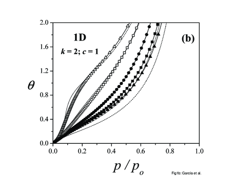
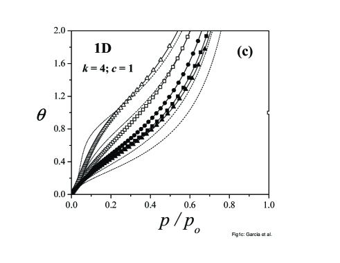
The effect of the -mer size on the adsorption isotherm can be understood by analyzing Figs. 1 (b) and 1 (c), where the study in Fig. 1 (a) is repeated for and , respectively. Two main conclusions can be drawn from the figures. Namely, the difference between the curves corresponding to different values of and the range of where the isotherms do not develop an inflection point diminish as is increased.
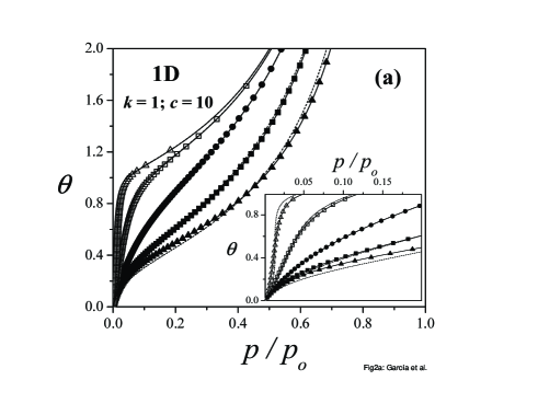
Figs. 2 and 3 show the effect of the parameter on the adsorption isotherms. As can be observed, all curves exhibit a pronounced knee as the parameter is increased. This effect can be better visualized in the insets of Figs. 2 and 3, where a zoom of the region of low pressure is presented. In the case of attractive interactions, the knee appears around and can be associated to the formation of the monolayer. In the case of repulsive interactions, -mers avoiding configurations with NN heads arrange in a structure of alternating particles separated by an empty site. Thus, for a given value of and strong repulsive interactions, a marked knee is found at .
To complete the discussion of Figs. 1-3, we evaluate the reaches and limitations of the two theoretical approximations studied. QCA leads to exact solution in 1D systems. Consequently, MC simulations in the grand canonical ensemble (symbols) fully agree with the predictions from QCA (solid lines), which reinforces the robustness of the two methodologies employed here. With respect to BWA, two different behaviors are observed : for small values of , the theoretical curves show a good agreement with the simulation data and for , appreciable differences are observed between BWA and MC results. For strong attractive couplings [see, for instance, the case corresponding to in Fig. 1 (a)], a characteristic van der Waals loop is observed in the adsorption isotherm and BWA incorrectly predicts a phase transition for . The shape of the isotherms is fairly independent of the size of the molecules. However, the disagreement between the BWA curves and the exact results turns out to be significantly large for larger -mer sizes [see, for instance, Fig. 1 (c)].
The analysis of the curves in Figs. 1-3 indicates that the appearance of a inflection point in the curves depends on , and . This will be studied in detail in the following. The point of inflection can be obtained in three steps: differentiating twice the adsorption isotherm equation to obtain (being for the sake of simplicity); equating the resulting expression to zero and solving for gives , the value of at the point of inflection; and inserting in the adsorption isotherm equation gives , the value of at the point of inflection.
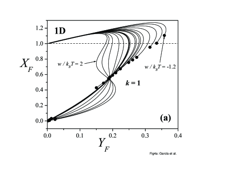
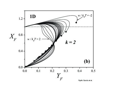
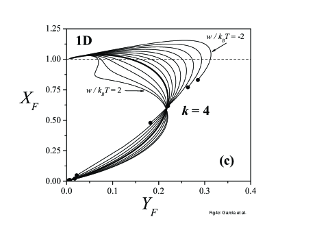
The location of the point of inflection () is plotted in Fig. 4 for different values of and . The information is organized as follows: as in Figs. 1-3, parts (a), (b) and (c) correspond to , and , respectively; the curves in (a), (b) and (c) were obtained for different values of (as indicated in the caption of each figure); and each point on a given curve corresponds to a determined value of .
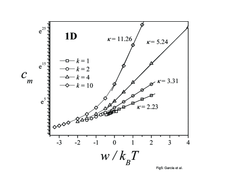
In order to understand the basic phenomenology, we consider in the first place the case corresponding to (highlighted curve). Clearly, the value of at the point of inflection may deviate considerably from unity. However, there exist a certain value of , where the point of inflection coincides with the point corresponding to the monolayer capacity. Fig. 5 shows the values of , obtained numerically, as a function of for four -mer sizes (). Two regimes can be clearly differentiated according to the sign of the lateral interactions. For attractive interactions, is not defined in all the range of . Thus, for each -mer size, there exists a limit value of the lateral interaction, , below of which the coordinate characterizing the inflection point in the adsorption isotherm is larger than one. In other words, the diagrams corresponding to values of below do not cross the line corresponding to (dashed line in Fig. 4). The values of for are collected in Table I. Finally, increases monotonically as the interaction energy is increased in the range . On the other hand, shows an exponential dependence [] in the range , where is a parameter depending on the -mer size. The different values of , obtained from the slope of vs. are reported in Table I.
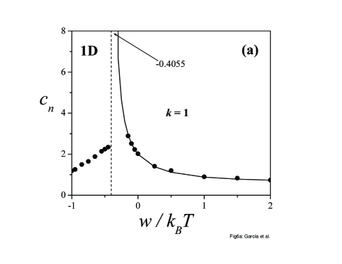
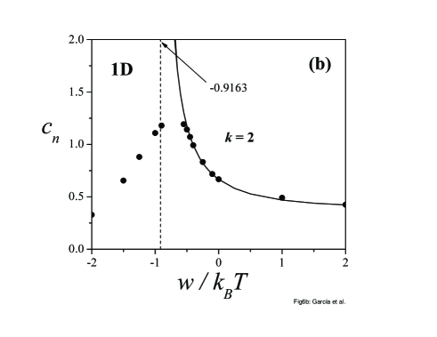
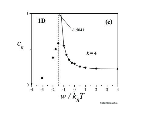
For values of between and infinity the adsorption at the point of inflection exceeds the monolayer capacity; for values of below the two quantities deviate more and more and for a limit value of , the point of inflection disappears444For , the isotherm is of Type II and when is less than the isotherm is of Type III and discussion of the point of inflection is meaningless.. In the low-coverage regime (), vs. can be calculated analytically (see Appendix for further discussion). The result of this calculation is presented in Fig. 6 for different values of . Solid lines represent theoretical data from Eq. (73) and symbols correspond to values of obtained numerically. As can be visualized from the figure, the dashed line separates two well differentiate regions. At right of the dashed line, the coordinates of the inflection point corresponding to the limit value are and . Then, the assumption of in Appendix is valid and the symbols coincide with the solid line. At left of the dashed line, the point of inflection disappears for and the solid line is not defined. The value of corresponding to the dashed line was obtained from the condition [see Eq. (73)]. From the point of view of the diagrams, the previous condition separates diagrams defined in the origin from those where the inflection point disappears for (see solid circles in Fig. 4).
In the next we will refer to one of the main applications of BET model, which consists in taking an experimental isotherm in the low-pressure region and fitting values of the monolayer volume and the parameter , from the linearized form of the BET equation,
| (35) |
The plot of vs should therefore be a straight line with slope and intercept . Solution of these two simultaneous equations gives and :
| (36) |
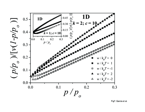
In this context, it is of interest to study the behavior of multilayer isotherms of -mers (with ) in the low-pressure region555Although in each particular case it is possible to find an optimum range of relative pressures, for practical purposes, we have chosen to set this range from to . Nevertheless, by choosing other ranges (for example, between and ) we obtain similar results. in comparison with BET isotherm. For this purpose, we will analyze, by using the standard BET formalism, exact theoretical isotherms in the 1D case. As an example, Fig. 7 shows the results obtained for , , and pressures ranging from up to . Symbols represent theoretical data from QCA (exact results) and lines correspond to linearized forms of the BET equation. A linear function is only obtained if and (see inset). The nonlinear behavior of interacting -mers isotherms at low pressures, which is a distinctive characteristic of many experimental isotherms, is showing that the polyatomic character of the adsorbate and the lateral interactions must be taken into account. The significant differences observed as and are varied indicate that the analysis of experimental isotherms of interacting larger molecules by means of the BET isotherm would lead to values of the parameters and appreciably different from the real ones.
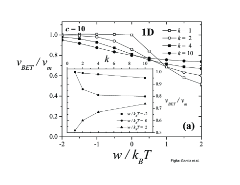
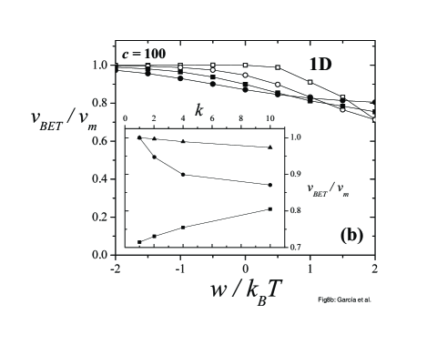
In order to measure the differences mentioned above, the analysis of Fig. 7 was repeated in Fig. 8 for [part (a)], [part (b)] and different values of and . The results obtained for the monolayer volume are shown in the figure, where and represent the real monolayer volume and the corresponding value obtained from the BET fitting, respectively. We start analyzing the case of (see inset). In this condition, the difference between and () increases (decreases) initially as the -mer size is increased and remains almost constant for larger values of . As is shown in the figure, these differences diminish as the parameter increases. Now, it is interesting to analyze the effect of the lateral interactions. As was discussed above, attractive lateral interactions favor the formation of the monolayer and, consequently, compensate the effect of the multisite occupancy. Thus, for a given value of , tends to one as is increased. On the other hand, repulsive interactions do not facilitate the formation of the monolayer, increasing the differences between and . For , a marked knee is found at and is close to this value of coverage. As the -mer size is increased, and, consequently, . This phenomenon can be clearly visualized by observing the curves corresponding to in the insets of Figs. 8 (a) and 8 (b).
3.2 Approximate solution in the 2D case
Because the structure of lattice space plays such a fundamental role in determining the statistics of -mers, it is of interest and of value to inquire how a specific lattice structure influences the main thermodynamic properties of adsorbed -mers. Following this line of thought, we use in this section the lattice-gas language again and assume the same model as in Subsection 3.1 with one exception: the sites form a 2D square lattice instead of a 1D lattice.
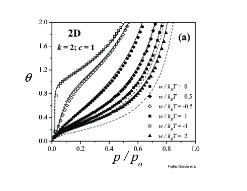
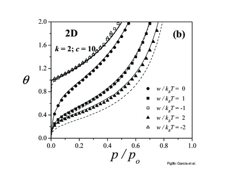
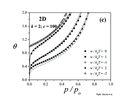
In Fig. 9 simulated isotherms are compared to theoretical ones from Eqs. (24), (26) and (31) for dimers adsorbed on 2D lattices with different values of and : (a), and ; (b) and ; and (c) and .
In the attractive case, the two theoretical approximations agree qualitatively well and the adsorption isotherms for BWA (dashed lines) and QCA (solid lines) are hardly distinguishable from each other. The differences between numerical and theoretical results can be much easily rationalized with the help of the absolute error, , which is defined as , where () represents the surface coverage obtained by using MC simulation (analytical approach). Each pair of values (, ) is obtained at fixed . The curves of vs (data are not shown here for sake of simplicity) indicate that, in all cases, QCA leads to appreciably better results than BWA.
Note that the stronger the lateral interaction, the more steep the adsorption isotherm becomes. This behavior could be indicative of the existence of a first-order phase transition at low temperatures. However, the study of the critical behavior of the system is out of the scope of the present work and will be object of future studies.
With respect to repulsive interactions, the differences between QCA and BWA are very appreciable. Beyond quantitative discrepancies, there exists qualitative differences between both approximations. Thus, while QCA is practically independent of , the discrepancies between BWA and MC results diminish appreciably for larger values of .
Summarizing, QCA gives a much better description of the 2D MC adsorption isotherms than the BWA. In the particular case of repulsive interactions, the disagreement between MC and BWA turns out to be significantly large, while QCA appears as the simplest approximation capable to take into account the main features of the multisite-occupancy adsorption. In fact, there exists a wide range of ’s (), where QCA provides an excellent fitting of the simulation data. In addition, most of the experiments in surface science are carried out in this range of interaction energy. Then, QCA not only represents a qualitative advance in the description of the multilayer adsorption of -mers with respect to the BWA, but also gives a framework and compact equations to consistently interpret thermodynamic adsorption experiments of polyatomics species such as alkanes, alkenes, and other hydrocarbons on regular surfaces.
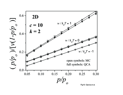
As indicated in the previous section, it is of interest to study the behavior of 2D multilayer isotherms (with ) in the low-pressure region in comparison with BET isotherm. For this purpose, the adsorption isotherms are plotted in the low-pressure regime and fitted with the linearized form of the BET equation. A typical example is shown in Fig. 10. The values of the parameters used in the figure are: , and . Open symbols represent Monte Carlo data, full symbols correspond to theoretical results obtained from QCA and lines correspond to linearized forms of the BET equation. As discussed in Fig. 9, QCA provides very good results in the limit of attractive lateral interactions and its accuracy diminishes for repulsive ad-ad interactions.
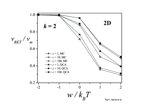
The analysis of Fig. 10 was repeated for different values of and . In all cases, the monolayer volume was calculated from the slope and intercept of the linearized form of the BET equation. The results are shown in Fig. 11. Several conclusions can be drawn from the figure: QCA agrees very well with the numerical results in all range of and studied; the differences between and diminish as the parameter increases; and attractive lateral interactions compensate the effect of the multisite occupancy. In other words, the behavior of vs is similar to the one described above for the 1D case.
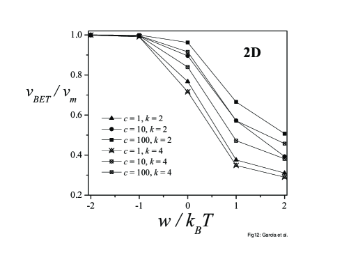
Finally, the effect of the -mer size on is analyzed in Fig. 12. In the figure, simulation results for (full symbols) are compared with the corresponding ones obtained for (crossed symbols). As can be observed, the behavior of vs does not significantly vary as the -mer size changes from to . In addition, the agreement between QCA and MC data (not shown here for sake of clarity) remains very good. Even though MC simulations of larger linear adsorbates on regular 2D lattices would be necessary to confirm the applicability of Eqs. (24) and (31), it should be pointed out that QCA is a good analytical approach considering the complexity of the physical situation which is intended to be described.
4 Conclusions
In this work, we have studied the multilayer adsorption of interacting polyatomic molecules. Two analytic isotherms were developed in the framework of the BWA and the QCA. The polyatomic character of the adsorbate was modelled by a lattice-gas of -mers. With respect to lateral interactions, the ad-ad couplings in the monolayer were explicitly considered in the solutions. The range of validity of both isotherms was analyzed by comparing theoretical and MC simulation results.
The new formalism from QCA leads to exact results in 1D and provides a close approximation to study multilayer adsorption of interacting polyatomics on 2D surfaces. On the other hand, the artificial effects that the BWA induces on the main thermodynamic functions can now be rationalized and compared with other analytical approaches. In this sense, we have shown that the disagreement between BWA and MC simulations increases as the temperature is decreased (or the ratio is increased) and the -mer size is increased.
In addition, we have studied the 1D and 2D BET plots obtained using the analytic and simulation isotherms. For non-interacting -mers, we found that the use of BET equation leads to an underestimate of the true monolayer volume: this volume diminishes as is increased. The situation is different for the case of interacting molecules. Thus, attractive lateral interactions favor the formation of the monolayer and, consequently, compensate the effect of the multisite occupancy. In this case, the monolayer volume predicted by BET equation agrees very well with the corresponding true value. In the case of repulsive couplings, the lateral interactions impede the formation of the monolayer and the BET predictions are bad (even worse than those obtained in the non-interacting case). Both the compensation effect for attractive interactions and the underestimation of the monolayer volume for repulsive interactions are more important for 2D systems.
5 ACKNOWLEDGMENTS
This work was supported in part by CONICET (Argentina) under project PIP 6294; Universidad Nacional de San Luis (Argentina) under project 322000; Universidad Tecnológica Nacional, Facultad Regional San Rafael (Argentina) under project PID PQCO SR 563 and the National Agency of Scientific and Technological Promotion (Argentina) under project 33328 PICT 2005. The numerical work were done using the BACO parallel cluster (composed by 60 PCs each with a 3.0 GHz Pentium-4 processor) located at Instituto de Física Aplicada, Universidad Nacional de San Luis-CONICET, San Luis, Argentina.
6 Appendix 1
In order to determine , we will use a similar scheme to that employed in Appendix A of Ref.[18]. Here, we restrict the analysis to 1D systems.
We start calculating the inflection point of the adsorption isotherm
| (37) |
By calculating the second derivative of in Eq. (24), we obtain:
| (38) |
where and represent and , respectively. Now, by taking in Eq. (38), which implies , the following relation is obtained:
| (39) |
The last equation allows us to obtain from the monolayer adsorption isotherm. At low density (), the virial expansion approach can be considered as an exact result [29]. As usual, can be written as a power series. Thus, by using Eq. (23),
| (40) |
Differentiating both sides of the last equation with respect to , we obtain
| (41) |
| (42) |
Note that as and, consequently, . By taking the limit as , Eq. (42) results
| (43) |
and
| (44) |
| (50) |
| (51) |
Then, by introducing Eqs. (50) and (51) in Eq. (47) and by using Eq. (44), we obtain
| (52) |
| (53) |
and
| (54) |
Finally, by introducing Eqs. (44) and (54) in Eq. (39), can be written in terms of and :
| (55) |
and
| (56) |
Now, we start with the calculation of and [29]. For this purpose, we write the first two terms of the grand partition function of a lattice-gas of -mers on sites,
| (57) |
where and represent the partition functions for one and two -mers, respectively.
By using the following expression,
| (58) | |||||
where is an arbitrary function, , and , can be written as
| (59) |
and the surface coverage results
| (60) | |||||
where the ’s are the well-known virial coefficients. In this case,
| (61) |
and
| (62) |
In addition, the relationship between the ’s and the ’s can be obtained by simple algebra. Thus,
| (63) |
and
| (64) |
On the other hand, and can be calculated as
| (65) |
and
| (66) |
where the configurational factors can be easily obtained. Thus,
| (67) |
| (68) |
Then,
| (69) |
| (70) |
| (71) | |||||
| (72) |
and, finally,
| (73) | |||||
References
- [1] T. L. Hill, An Introduction to Statistical Thermodynamics, Addison Wesley Publishing Company, Reading, MA, 1960.
- [2] A. Clark, The Theory of Adsorption and Catalysis, Academic Press, New York and London, 1970.
- [3] W. A. Steele, The interaction of gases with solid surfaces, Pergamon Press, New York, 1974.
- [4] A.W. Adamson, Physical Chemistry of Surfaces, John Wiley and Sons, New York, 1990.
- [5] W. Rudziński and D. Everett, Adsorption of Gases on Heterogeneous Surfaces, Academic Press, New York, 1992.
- [6] I. Langmuir, J. Am. Chem. Soc. 40 (1918) 1361.
- [7] S. Brunauer, P.H. Emmet, E. Teller, J. Am. Chem. Soc. 60 (1938) 309.
- [8] S.J. Gregg, K.S.W. Sing, Adsorption, Surface Area, and Porosity, Academic Press, New York, 1991.
- [9] P. J. Flory, J. Chem. Phys. 10 (1942) 51. P. J. Flory, Principles of Polymers Chemistry, Cornell University Press, Ithaca, NY, 1953.
- [10] M. L. Huggins, J. Phys. Chem. 46 (1942) 151. M. L. Huggins, Ann. N.Y. Acad. Sci. 41 (1942) 1. M. L. Huggins, J. Am. Chem. Soc. 64 (1942) 1712.
- [11] E. A. Guggenheim, Proc. R. Soc. London A183 (1944) 203.
- [12] E. A. DiMarzio, J. Chem. Phys. 35 (1961) 658.
- [13] T. Nitta, M. Kuro-oka, T. Katayama, J. Chem. Eng. Jpn. 17 (1984) 45.
- [14] W. Rudziński, K. Nieszporek, J. M. Cases, L. I. Michot, F. Villieras, Langmuir 12 (1996) 170.
- [15] G. L. Aranovich, M. D. Donohue, J. Colloid Interface Sci. 175 (1995) 492.
- [16] G. L. Aranovich, M. D. Donohue, J. Colloid Interface Sci. 189 (1997) 101.
- [17] J. L. Riccardo, A. J. Ramirez-Pastor, F. Romá, Langmuir 18 (2002) 2130.
- [18] F. Romá, A. J. Ramirez-Pastor, J. L. Riccardo, Surf. Sci. 583 (2005) 213.
- [19] E. Ising, Z. Physik 31 (1925) 253.
- [20] C. Domb, in: C. Domb, M.S. Green (Eds.), Phase transitions and critical phenomena, Academic Press, London-New York, 1974, Vol. 3, pp. 1-95; M.E. Fisher, Rep. Prog. Phys. 30 (1967) 731.
- [21] L. Onsager, Physical Review 65 (1944) 117.
- [22] H. Bethe, Proc. R. Soc. London A150 (1935) 552.
- [23] P.J. Flory, J. Chem. Phys. 10 (1942) 51.
- [24] P.J. Flory, Principles of Polymers Chemistry, Cornell University Press, Ithaca N.Y., (1953).
- [25] A. J. Ramirez-Pastor, T. P. Eggarter, V. D. Pereyra, J. L. Riccardo, Phys. Rev. B 59 (1999) 11027.
- [26] A. J. Ramirez-Pastor, J. L. Riccardo, V. Pereyra, Langmuir 16 (2000) 10167.
- [27] M. Dávila, F. Romá, J. L. Riccardo, A. J. Ramirez-Pastor, Surf. Sci. 600 (2006) 2011.
- [28] N. Metropolis, A.W. Rosenbluth, M.N. Rosenbluth, A.H. Teller, E. Teller, J. Chem. Phys. 21 (1953) 1087.
- [29] F. Romá, A. J. Ramirez-Pastor, J. L. Riccardo, Langmuir 19 (2003) 6770.
| -mer size | ||
|---|---|---|
| = 1 | ||
| = 2 | ||
| = 4 | ||
| = 10 |