Signal Processing for Pico-second Resolution Timing Measurements

Abstract

The development of large-area homogeneous photo-detectors with sub-millimeter path lengths for direct Cherenkov light and for secondary-electrons opens the possibility of large time-of-flight systems for relativistic particles with resolutions in the pico-second range. Modern ASIC techniques allow fast multi-channel front-end electronics capable of sub-pico-second resolution directly integrated with the photo-detectors. However, achieving resolution in the pico-second range requires a precise knowledge of the signal generation process in order to understand the pulse waveform, the signal dynamics, and the noise induced by the detector itself, as well as the noise added by the processing electronics. Using the parameters measured for fast photo-detectors such as micro-channel plates photo-multipliers, we have simulated and compared the time-resolutions for four signal processing techniques: leading edge discriminators, constant fraction discriminators, multiple-threshold discriminators and pulse waveform sampling.

1 Introduction

The typical resolution for measuring time-of-flight of relativistic particles achieved in large detector systems in high energy physics has not changed in many decades, being on the order of 100 psec [1, 2]. This is set by the characteristic scale size of the light collection paths in the system and the size of the drift paths of secondary electrons in the photo-detector itself, which in turn are usually set by the transverse size of the detectors, characteristically on the order of one inch (100 psec). However, a system built on the principle of Cherenkov radiation directly illuminating a photo-cathode followed by a photo-electron amplifying system such as a Micro-Channel Plate Photo-Multiplier (MCP-PMTs) [3] with characteristic dimensions of 10 microns or less, has a much smaller characteristic size, and consequently a much better intrinsic time resolution [4, 5, 6].

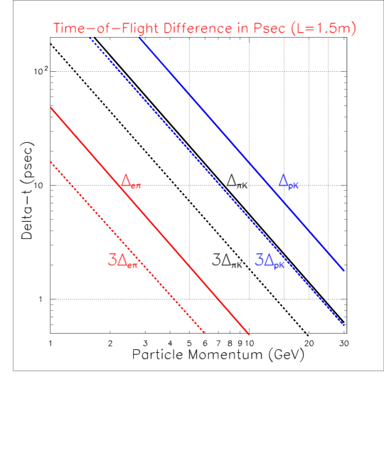
Figure 1: The difference in times (solid lines) over a path-length of 1.5m for electrons (i.e. zero time delay relative to the speed of light) versus pions, pions versus kaons, and kaons versus protons, as a function of the charged particle momentum. The time resolutions necessary for a 3-$\sigma$ separation versus momentum are also shown (dashed lines).

Time-of-flight techniques with resolution of less than several picoseconds would allow the measurement of the mass, and hence the quark content, of relativistic particles at upgraded detectors at high energy colliders such as the Fermilab Tevatron, the LHC, Super-B factories, and future lepton-colliders such as the ILC or a muon-collider, and the association of a photon with its production vertex in a high-luminosity collider [7]. Other new capabilities at colliders would be in associating charged particles and photons with separate vertices in the 2-dimensional time-vs-position plane, and searching for new heavy particles with short lifetimes [8, 9]. The difference in transit times over a path-length of 1.5 meters, typical of the transverse dimension in a solenoidal collider detector such as CDF or ATLAS, is shown in Figure 1. Many other applications with different geometries, such as forward spectrometers, would have significantly longer path-lengths, with a consequent reach in separation to higher momenta, as can be scaled from the figure.

There are possible near-term applications of fast timing requiring resolutions of several picoseconds but smaller area systems ($\simeq$0.001-1 m²), such as missing-mass searches for the Higgs at the LHC [10], and non-magnetic spectrometers for the development of 6-dimensional phase-space muon cooling [11]. There are likely to be applications in other fields as well, such as measuring longitudinal emittances in accelerators, precision time-of-flight in mass spectroscopy in chemistry and geophysics, and applications in medical imaging.

At lower time and position resolution, the same techniques could be used for instrumenting the surfaces of large-ring imaging water Cherenkov counters, in which measurement of both the position and time-of-arrival of Cherenkov photons would allow reconstruction of track directions and possibly momenta [12].

In order to take advantage of photo-detectors with intrinsic single photo-electron resolutions of tens of picoseconds to build large-area time-of-flight systems, one has to solve the problem of collecting signal over distances large compared to the time resolution while preserving the fast time resolution inherent in the small feature size of the detectors themselves. Since some of these applications would cover tens of square meters and require tens of thousands of detector channels, the readout electronics have to be integrated via transmission lines with the photo-detector itself in order to reduce the physical dimensions and power, increase the analog band-width, improve readout speed, and provide all-digital data output.

There are a number of techniques to measure the arrival time of very fast electrical pulses [13, 14, 15, 16]. Typically one measures the time at which the pulse crosses a single threshold, or, for better resolution, the time at which the pulse reaches a constant fraction of its amplitude [17]. An extension of the threshold method is to measure the time that a pulse crosses multiple thresholds [18].

A recent development is the large-scale implementation of fast analog waveform sampling onto arrays of storage capacitors using CMOS integrated circuits at rates on the order of a few GSa/s. Most, if not all of them, have actually 3dB analog bandwidths below 1 GHz  [19, 20, 21, 22]. The steady decrease in feature size and power for custom integrated circuits now opens the possibility for multi-channel chips with multi-GHz analog bandwidths, and able to sample between 10 and 100 GHz, providing both time and amplitude after processing. Assuming that the signals are recorded over a time interval from before the pulse to after the peak of the pulse, with sufficient samples fast waveform sampling provides the information to get the time of arrival of the first photo-electrons, the shape of the leading edge, and the amplitude and integrated charge. While other techniques can give time, amplitude, or integrated charge, fast sampling has the advantage that it collects all the information, and so can support corrections for pileup, baseline shifts before the pulse, and filtering for noisy or misshapen pulses. In applications such as using time-of-flight to search for rare slow-moving particles, having the complete pulse shape provides an important check that rare late pulses are consistent with the expected waveform.

The outline of this note is as follows: Section 2 describes the four techniques for determining the time-of-arrival of an electrical pulse from a photo-detector. Section 3 describes the input signal parameters of the simulation program used for the comparisons, and the parameters used for each of the four methods in turn. Section 4 presents the results and the methods and parameters to be used in real systems. The conclusions and summary are given in Section 5.

2 Timing techniques

Present photo-detectors such as micro-channel plate photo-multipliers (MCP-PMTs) and silicon photomultipliers achieve rise-times well below one nanosecond [23, 24, 25]. Ideal timing readout electronics would extract the time-of-arrival of the first charge collected, adding nothing to the intrinsic detector resolution. Traditionally the best ultimate performance in terms of timing resolution has been obtained using constant fraction discriminators (CFDs) followed by high precision amplitude digitization. However, these discriminators make use of wide-band delay lines that cannot be integrated easily into silicon integrated circuits, and so large front-end readout systems using CFD’s to achieve sub-nsec resolution have are not yet been implemented.

Several other well-known techniques in addition to constant-fraction discrimination have long been used for timing extraction of the time-of-arrival of a pulse:

1. Single threshold on the leading edge;

2. Multiple thresholds on the leading edge, followed by a fit to the edge shape;

3. Pulse waveform sampling, digitization and pulse reconstruction.

Applying a fixed threshold to the leading edge, which is a one-parameter technique, suffers from a dependence of the extracted time with the pulse amplitude, even for identical waveforms. In addition, this method is sensitive to base-line shifts due to ‘pile-up’, the overlap of a pulse with a preceding one or many, a situation common in high-rate environments such as in collider applications. Also, for applications in which one is searching for rare events with anomalous times, the single measured time does not give indications of possible anomalous pulse shapes due to intermittent noise, rare environmental artifacts, and other real but rare annoyances common in real experiments.

In contrast, constant fraction discrimination takes into account the pulse amplitude. The most commonly used constant fraction discriminator technique forms the difference between attenuated and delayed versions of the original signal. There are therefore three parameters: the delay, the attenuation ratio, and the threshold. These parameters have to be carefully set with respect to the pulse characteristics in order to obtain the best timing resolution.

The multiple threshold technique samples the leading edge at amplitudes set to several values, for instance at values equally spaced between a minimum and a maximum threshold. The leading edge is then reconstructed from a fit to the times the pulse reaches the thresholds to extract a single time as characteristic of the pulse. As in the case of constant fraction discrimination, if the pulse shape is independent of amplitude, the reconstructed time will also not depend upon the pulse amplitude, provided the thresholds are properly set.
In the simulation, the single threshold was set at 8$\%$ of the average pulse amplitude, providing the best timing resolution. Lower threshold values could not be used due to the noise, particularly at low photo-electrons numbers. For multiple-threshold, almost no improvement was found at more than four thresholds; the lowest and highest thresholds were determined to avoid sensitivity and inefficiencies at low photo-electrons numbers.

Waveform sampling stores successive values of the pulse waveform. For precision time-of-arrival measurements, such as considered here, one needs to fully sample at least the leading edge over the peak. In order to fulfill the Shannon-Nyquist condition  [26], the sampling period has to be chosen short enough to take into account all frequency components containing timing information, which is that the minimum sampling frequency is set at least at twice the highest frequency in the signal’s Fourier spectrum. In practice, there are frequency components contributing to the leading edge well above the 3-dB bandwidth of the signal spectrum, before the noise is dominant, and these components should not be filtered out. After digitization, using the knowledge of the average waveform, pulse reconstruction allows reconstructing the edge or the full pulse with good fidelity. The sampling method is unique among the four methods in providing the pulse amplitude, the integrated charge, and figures of merit on the pulse-shape and baseline, important for detecting pile-up or spurious pulses.

3 Simulations

We have developed a Monte-Carlo simulation tool using MATLAB [27] in order to generate pulses having the temporal and spectral properties of fast photo-detector signals, and to simulate and compare the behavior of the four techniques described in Section II. Both amplitude and timing resolution are estimated as a function of various parameters, such as the number of photo-electrons, the signal-to-noise ratio, and the analog bandwidth of the input section of the front-end electronics [28]. In the case of sampling, the resolution is estimated as a function of the sampling frequency, the number of bits in the analog-to-digital conversion, and the timing jitter of the sampling. The four methods are simulated and results are evaluated with respect to each other below.

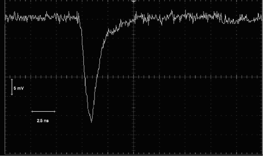
Figure 2: A signal from a Photonis XP85011 micro-channel plate photo-detector with $25\mu$-diameter pores [29], recorded with a Tektronix TDS6154C oscilloscope [30], using the ANL laser test-stand [31]. Signal to Noise ratio is 40. The oscilloscope analog bandwidth is 15 GHz, sampling rate 40 GS/s, and the horizontal and vertical scales are 2.5 ns/division, and 5mV/division, respectively.

3.1 Input signals

In order to run a Monte-Carlo using realistic signals, pulses have been synthesized based on measurements of MCP signals such as those shown in Figure 2. The synthesized signals are calculated as the convolution of a triangular waveform having a rise time of 100 ps and fall time on the same order [23], with an impulse waveform of $\tau e^{-t/\tau}$, where $\tau$ is set according to the analog bandwidth of the front-end electronics. With a 1.5 GHz analog bandwidth, $\tau$ is set to 235 ps. This waveform is then convolved with itself, in order to match the MCP pulse shape. The simulated input signals have variable spread in amplitude, implemented by taking into account the number of incident photo-electrons, ${N_{pe}}$, as normally distributed with $\sigma$ proportional to $1/\sqrt{N_{pe}}$. To average over discrete binning effects, we introduce a spread in the initial time, distributed uniformly between +$\tau$ and –$\tau$.

The simulation includes both detector shot noise and thermal noise superimposed on the signal. The noise is taken with two contributions:

1. white shot noise from the MCP, which is then shaped by the electronics in the same way as is the MCP output signal;

2. white thermal noise is assumed to originate from the electronics components.

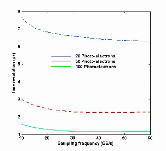
Figure 3: Typical synthesized MCP-PMTs signals used in the simulation for an input signal of 50 photo-electrons. To average over discrete binning effects, signals are spread in the initial time, distributed uniformly between +$\tau$ and –$\tau$.

These two noise spectra are weighted so that they contribute equally to the overall signal-to-noise ratio.

A set of 300 synthesized signals with a mean of 50 photo-electrons, assuming a 1.5 GHz analog bandwidth, is shown in Figure 3. Figure 4 displays the Fourier spectra of: a)a noiseless MCP signal, b) MCP shot noise, c) electronics noise, and d) the final noisy MCP signal, including both sources of noise, for 20 input photo-electrons, and an overall bandwidth of 1.5 GHz. The signal-to-noise ratio is taken to be 32.

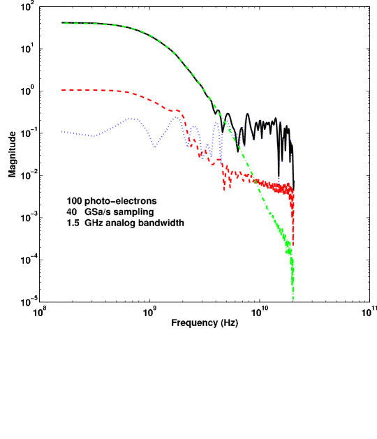
Figure 4: Fourier spectra of a synthesized noiseless MCP signal (green, dashed-dots), MCP shot noise (red, dashed), electronics noise (blue, dots), and the final ‘noisy’ MCP signal with both sources of noise included (black, solid). Sampling rate is set at 40 GSa/s, therefore, all frequency components above 20 GHz have been removed with an anti-aliasing filter.

3.2 Simulation of the Leading Edge Discriminator

In the simulation the fully-simulated waveform (i.e. with noise added as described above) is intersected with a threshold set at the value providing the best timing resolution for a given set of external parameters, such as the analog bandwidth, or the number of photo-electrons. For comparison with actual threshold measurements, some overdrive effects should probably be considered. The comparators are assumed to be ideal, i.e. the trigger is generated by the first time step in the simulation that has a pulse amplitude over the ‘arming’ threshold. The threshold is set between 4% and 15% of the average amplitude pulse height.

3.3 Simulation of the Multi-Threshold Discriminator

The multiple threshold technique [18] intersects the input waveform with several thresholds, typically (but not necessarily) equally spaced between a minimum and a maximum. A fit is then performed, and a single time is extracted as the time-of-arrival of the pulse. Figure 5 shows an example, with the best-fit time taken as the intersection of the fit extrapolated to the intersection with the time axis. For the input parameters we have chosen, we find that four thresholds, equally spaced between 10 and 50% of the average pulse height, are enough so that more thresholds do not significantly improve the performance.

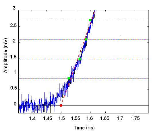
Figure 5: An example of the multi-threshold simulation and technique. Green dots: crossed thresholds, red dots: zero-crossing time from the extrapolation of the fit (red line) to the nominal start of the pulse at zero amplitude.

3.4 Simulation of the Constant Fraction Discriminator

A constant fraction discriminator fires at a fixed fraction of the amplitude of the pulse, relying on the assumption that the pulse shape is independent of amplitude. The implementation considered here is that the input pulse is attenuated between 30 and 40%, inverted, and then summed with a version of the pulse delayed between 150 and 200 picoseconds. If the pulse passes a predetermined ‘arming’ threshold, set in the simulations to between 10 and 20% of the average pulse height, the time of the zero-crossing of the summed pulse is measured. As in the case of the leading edge simulation, the parameters are optimized to get the best possible timing resolution for a given set of parameters.

3.5 Simulation of Pulse Waveform Sampling

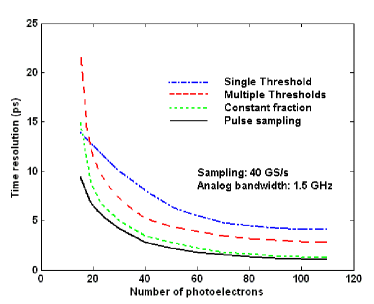
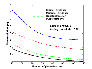
Figure 6: Left: Time resolution versus the number of primary photo-electrons, for the four different timing techniques: one-threshold (blue, dashed-dots), constant fraction (green, dots), multiple threshold (red, dashed), and waveform sampling (black, solid) at 40 GSa/s. The analog bandwidth of the input to the sampling is taken to be 1.5 GHz, no sampling jitter added. Right: The same plot with the abscissa expanded to cover from 40 to 110 photo-electrons, and the ordinate expanded to cover 1 to 9 ps.

The simulation of pulse waveform sampling performs a number of samples of the signal voltage at equally spaced time intervals, digitized with a given precision in amplitude corresponding to the number of bits assumed in the A-to-D conversion, and adds a random jitter in the time of each sample. Sampling rates between 10 and 60 GSa/s have been simulated for A-to-D conversion precisions of between 4 and 16-bits. The analog bandwidth of the MCP device and associated front-end electronics are included in the simulations.

An iterative least-squares fit to a noiseless MCP template signal is then applied to the data using the Cleland and Stern algorithm that has been implemented for high resolution calorimetry measurements with Liquid Argon [32] .

4 Results of the Simulations

Figure 5 shows the time resolution versus the number of photo-electrons for the four timing techniques. The number of photo-electrons is varied between between 15 and 110; the sampling rate is 40 GSa/s, with no sampling jitter. The analog bandwidth is assumed to be 1.5 GHz, and in the case of sampling, the digitization is taken to have a precision of 16 bits.

The waveform sampling technique performs best of the four techniques, particularly for lower numbers of photo-electrons. Note that the sampling technique is relatively insensitive to (random) clock jitter; at 40 GSa/s sampling; jitters smaller than 5 psec do not introduce significant degradation in the resolution [33, 34].

Table 1 shows the timing resolution for each technique for a set of parameters we have chosen as a base-line for use in a future detector: an input signal of 50 photo-electrons, a 1.5 GHz analog bandwidth, and for each technique, a signal-to-noise ratio of 80. All Monte-Carlo simulations were run with 300 events; the corresponding statistical uncertainty is on the order of 5%.

Technique	Resolution
	(ps)
Leading Edge	7.1
Multiple Threshold	4.6
Constant Fraction	2.9
Sampling	2.3

Table 1: The predicted timing resolution for each technique for an assumed input signal of 50 photo-electrons, a 1.5 GHz analog bandwidth, and a signal-to-noise ratio of 80. No sampling jitter has been added. The statistical uncertainty on each result is on the order of 5%.

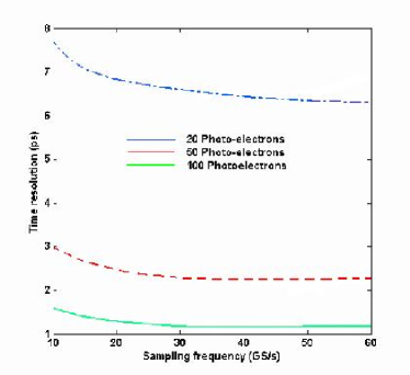
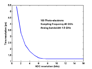
Figure 7: Pulse waveform sampling simulation results. Left: Time resolution versus sampling rate. The input signals correspond to 20, 50 and 100 photo-electrons. The digitization precision is 16-bits, with no sampling jitter added. The analog bandwidth is taken to be 1.5 GHz. Right: The timing resolution as a function of the number of bits used in the digitization. The sampling rate is 40 GSa/s, the analog bandwidth is 1.5 GHz. The signal is taken to be 100 photo-electrons, with a signal-to-noise ratio of 164. No sampling jitter has been added.

As expected, the multiple threshold technique is a clear improvement compared to the one-threshold discriminator for input signals above 10 photo-electrons. The constant fraction discriminator also is a significant improvement over a single-threshold for any input signal. However, the best method is waveform sampling, which achieves resolutions below 3 picoseconds for input signals of 50 photo-electrons in the base-line case of a S/N ratio of 80, 1.5 GHz analog input bandwidth, and random sampling jitter less than 5 psec.

Figure 7 shows the sensitivity of sampling to the digitization. The curve flattens out such that an 8-bit digitization is sufficient to get a resolution of a few picoseconds at a 40 GSa/s sampling rate. This greatly relaxes the constraints on the analog- to-digital converter design (we note that the A-to-D conversion does not have to be fast- the sampling is at 40 GSa/s, but the digitization rate is set by the occupancy requirements of the application, and for the small pixel sizes we are considering for most time-of-flight applications the digitization can be done in real time at rates below 1 MHz).

We have simulated the dependence of the time resolution with the analog bandwidth for our baseline sampling rate of 40 GSa/s, as shown in the left-hand plot of Figure 8. The time resolution versus analog bandwidth for a sampling rate proportional to the analog bandwidth is shown in the right-hand plot of Figure 8. In both cases, the time resolution improves with the analog bandwidth as expected, but flattens above a 2 GHz analog bandwidth and a 80 GSa/s sampling rate, showing that there is not much to gain in designing electronics beyond these limits.

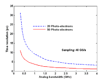
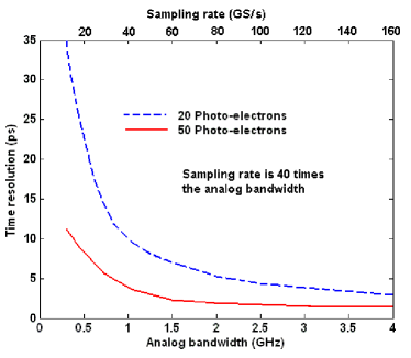
Figure 8: Pulse waveform sampling simulation results. Left: Time resolution versus analog bandwidth for a fixed sampling rate of 40 GSa/s, for input signals of 20 and 50 photo-electrons and an 8-bit A-to-D precision. Right: Time resolution versus analog bandwidth for a sampling rate proportional to the analog bandwidth, with 8-bit digitization and a 2-ps timing jitter.

The waveform sampling technique is also robust against random sampling clock jitter provided there are enough samples on the leading edge, as shown Figure 9.

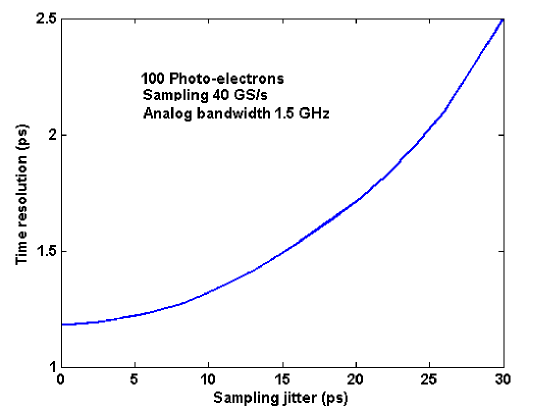
Figure 9: Right: Time resolution vs sampling jitter for input signals of 100 photo-electrons. The sampling rate is 40 GSa/s, the analog bandwidth is 1.5 GHz, and the digitization is assumed to be with a 16-bit ADC.

5 Summary and Conclusions

We have developed a simulation package based on MATLAB to model the time resolution for fast pulses from photo-detectors. Using the parameters measured from commercial micro-channel plate photo-multipliers, we have simulated and compared the time-resolutions for four signal processing techniques: leading edge discriminators, constant fraction discriminators, multiple-threshold discriminators and pulse waveform sampling. We find that timing using pulse waveform sampling gives the best resolution in many cases, particularly in the presence of white noise and a substantial signal, such as fifty photo-electrons. With micro-channel plate photo-detectors, our simulations predict that it should be possible to reach a precision of several picoseconds or better with pulse waveform sampling given large-enough input signals. At high sampling rates of the order of 40 GSa/s, a relatively low precision digitization (8-bit) can be used.

6 Acknowledgments

We are indebted to Dominique Breton, Eric Delagnes, Stefan Ritt, and their groups working on fast waveform sampling. We thank John Anderson, Karen Byrum, Chin-Tu Chen, Gary Drake, Camden Ertley, Daniel Herbst, Andrew Kobach, Jon Howorth, Keith Jenkins, Chien-Min Kao, Patrick Le Du, Tyler Natoli, Rich Northrop, Erik Ramberg, Anatoly Ronzhin, Larry Ruckman, Andrew Wong, David Salek, Greg Sellberg, Scott Wilbur, and Jerry Va’Vra for valuable contributions. We thank Paul Hink and Paul Mitchell of Burle/Photonis for much help with the MCP’s, and Larry Haga of Tektronix Corporation for his help in acquiring the Tektronix TDS6154C 40 GSa/s sampling oscilloscope on which much of this work is based. This work was supported in part by the University of Chicago, the National Science Foundation under grant number 5-43270, and the U.S. Department of Energy Advanced Detector Research program.

References

- [1] See, for example, D. Acosta et al. (CDF Collaboration); The Performance of the CDF Luminosity Monitor. Nucl. Instr. Meth. A518 (2004) 605-608.
- [2] W. Klempt. Review of Particle Identification by Time of Flight techniques. Nucl. Instr. Meth. A433 (1999) 542-553.
- [3] J.L. Wiza. Micro-channel Plate Detectors. Nucl. Instr. Meth. 162 (1979) 587-601.
- [4] T. Credo, H. Frisch, H. Sanders, R. Schroll, F. Tang. Picosecond Time of Flight for Particle Identification at High Energy Physics Colliders. Proceedings of the Nuclear Science Symposium, Rome (2004), 586.
- [5] K. Inami, N. Kishimoto, Y. Enari, M. Nagamine, and T. Ohshima. Timing properties of MCP-PMT. Nucl. Instr. Meth. A560 (2006) 303-308.
- [6] J. Va’vra, J. Benitez, J. Coleman, D. W. G. Leith, G. Mazaher, B. Ratcliff and J. Schwiening. A 30 ps Timing Resolution for Single Photons with Multi-pixel Burle MCP-PMT. Nucl. Instr. Meth. A572 (2007) 459-462.
- [7] At a high luminosity machine such as the LHC there are many collisions per beam crossing, making associating photons from a Higgs decay with a specific vertex difficult, to pick one example. This application would require the conversion of the photon and a simultaneous precision measurement of the time and position.
- [8] See, for example, C.H. Chen and J. F. Gunion. Probing Gauge-Mediated Supersymmetry Breaking Models at the Tevatron via Delayed Decays of the Lightest Neutralino. Phys. Rev. D 58 075005 (1998).
- [9] T. Aaltonen et al (CDF Collaboration). ArXiv: 0804.1043 [hep-ex], submitted to Phys. Rev. D.
-
[10]
See, for example,
http://hepwww.rl.ac.uk/accel/forum/2007/Cosenerswattsapr07.pdf - [11] The MANX Project Proposal https://mctf.fnal.gov/meetings/2007-1/04_05/project-narrative-06er86282-6dmanx-v2-w-appendices.pdf/view
- [12] Howard Nicholson, private communication.
- [13] D.I. Porat Review Of Sub-nanosecond Time Interval Measurements; IEEE Trans. Nucl. Sci. 20 (1973) 36.
- [14] J.F. Genat. High Resolution Time to Digital Converters. Nucl. Inst. Meth. A315 (1992) 411-414.
- [15] J. Kalisz Review of Methods for Time Interval Measurements with Picosecond Resolution, Institute of Physics Publishing, Metrologia, 41 (2004) 17-32; http://www.iop.org/EJ/abstract/0026-1394/41/1/004
- [16] An extensive list of references on timing measurements can be found in: A. Mantyniemi, MS Thesis, Univ. of Oulu, 2004; ISBN 951-42-7460-I; ISBN 951-42-7460-X; http://herkules.oulu.fi/isbn951427461X/isbn951427461X.pdf
- [17] S. Cova et al. Constant Fraction Circuits for Picosecond Photon Timing with Micro-channel Plate Photomultipliers. Review of Scientific Instruments, 64-1 (1993) 118-124.
- [18] H. Kim et al. Electronics Developments for Fast Timing PET Detectors. Symposium on Radiation and Measurements Applications. June 2-5 (2008), Berkeley CA, USA.
- [19] D. Breton, E. Auge, E. Delagnes, J. Parsons, W Sippach, V. Tocut. The HAMAC rad-hard Switched Capacitor Array. ATLAS note. (2001).
- [20] E. Delagnes, Y. Degerli, P. Goret, P. Nayman, F. Toussenel, and P. Vincent. SAM : A new GHz sampling ASIC for the HESS-II Front-End. Cerenkov Workshop (2005)
- [21] S. Ritt. Design and Performance of the 5 GHz Waveform Digitizer Chip DRS3. Submitted to Nuclear Instruments and Methods, (2007).
- [22] G. Varner, L.L. Rudman, A. Wong. The First version Buffered Large Analog Bandwidth (BLAB1) ASIC for high Luminosity Colliders and Extensive Radio Neutrino Detectors. Nucl. Inst. Meth. A591 (2008) 534.
- [23] J. Milnes and J. Howorth, Photek Ltd; Proc. SPIE 5580 (2005) 730-740.
- [24] K. Inami. Timing properties of MCP-PMTs. Proceedings of Science. International Workshop on new Photon-Detectors, June 27-29 (2007). Kobe University, Japan.
- [25] G.Bondarenko, B. Dolgoshein et al. Limited Geiger Mode Silicon Photodiodes with very high Gain. Nuclear Physics B, 61B (1998) 347-352.
- [26] C.E. Shannon. A Mathematical Theory of Communication. The Bell System Technical Journal, 27 (1948) 379-423 623-656.
- [27] MathWorks, 3 Apple Hill Drive, Natick, MA, USA. The MATLAB source is available from the authors.
- [28] The signal-to-noise ratio is defined as the ratio of the maximum of the amplitude of the pulse to the rms amplitude of the noise. The analog-bandwidth is defined as the frequency at which the system response has dropped by 3-db.
- [29] Photonis/Burle Industries, 1000 New Holland Av, Lancaster PA, 17601.
- [30] Tektronix INC, PO Box 500, Beaverton, OR 97977.
- [31] C. Ertley, J. Anderson, K. Byrum, G. Drake, E. May. http://www.hep.anl.gov/ertley/windex.html
- [32] W.E. Cleland and E.G. Stern. Signal Processing considerations for Liquid Ionization Calorimeters in a High Rate Environment. Nucl. Instr. Meth. A338 (1994) 467-497.
- [33] K.A. Jenkins, A.P. Jose, D.F Heidel An On-chip Jitter Measurement Circuit with Sub-picosecond Resolution. Proceedings of the 31st European Solid State Circuits Conference, 12 (2005) 157-160.
- [34] Systematic errors in sampling may be calibrated out with the use of extra calibration channels in the front-end readout.